Article

Study on Amplitude and Flatness Characteristics of Elastic Thin Strip under Fluid–Structure Interaction Vibration Excited by Unsteady Airflow

School of Mechanical Engineering, University of Science and Technology Beijing, Beijing 100083, China
*
Author to whom correspondence should be addressed.
Metals 2019, 9(5), 496; https://doi.org/10.3390/met9050496
Submission received: 22 March 2019 / Revised: 26 April 2019 / Accepted: 26 April 2019 / Published: 28 April 2019
(This article belongs to the Special Issue Researches and Simulations in Steel Rolling)

Abstract

:
Based on unsteady airflow excitation and elastic thin strip vibration theory, a SI-FLAT flatness meter was taken as the research object, and an amplitude–residual stress simulation analysis model of the cold rolling strip under aerodynamic loads was established by using ANSYS Workbench. First, the influences of fluid–structure interaction on the strip amplitude distribution and the flatness calculation deviation were analyzed. It was found that the analysis with fluid–structure interaction matched the actual measurement of the flatness meter better. Then, the influences of different aerodynamic loads and tensions on the strip midpoint amplitude and the flatness calculation deviation were analyzed. It was found that when alternating aerodynamic loads increased, the strip amplitude increased in the form of a quadratic polynomial. However, when the tensions decreased, the strip amplitude decreased exponentially. The strip dimensions also influenced the amplitude of vibration: The wider and thinner the strip, the larger the amplitude. Finally, the influences of different flatness defects on the strip amplitude distribution and the flatness calculation deviation were analyzed. The deviation was serious on the strip edge, and the fluctuation characteristics of the deviation were opposite to those of the initial flatness defects.

1. Introduction

Strip flatness, which is the core of flatness control in cold rolling, is one of the most important quality indexes of the cold rolling strip. Flatness control concretely includes flatness real-time measuring, flatness defect distinguishing, and flatness control parameter adjustment [1]. Flatness real-time measuring, which is the first important part of flatness control in cold rolling, is the core foundation in guaranteeing the flatness quality of the cold rolling strip. The large tension in cold rolling generally avoids the appearance of visible waves in the strip. Thus, flatness is usually detected by measuring the difference in tensile stress along the strip width. The contact flatness measuring roll is widely applied, but its measuring accuracy is influenced and its sensors are damaged when working in a bad environment, especially because of the intrusion of water, oil, and other media. Moreover, the flatness measuring roll is expensive, and the maintenance and regrinding of the roll face are difficult. Thus, these shortcomings have made the noncontact flatness meter a research hotspot in recent years [2]. Based on the principle of airflow excitation–eddy current amplitude measurement, the SI-FLAT noncontact flatness meter was successfully developed by Siemens in 1998. By imposing the excitation airflow of pulsation over time on the strip through the air pump and air conditioner, the strip is subjected to forced vibration. Then, the forced vibration amplitude is measured by the eddy current sensors. Finally, the strip flatness is calculated by the transformation model of the amplitude and flatness. At present, the SI-FLAT flatness meter has already become the most successful one [3,4]. As for the SI-FLAT flatness meter, the measurement of the strip amplitude distribution and the accuracy of the transformation model directly affect the measuring results. Yang et al. [5] simplified the strip vibration into a Euler beam vibration based on an analysis of the flatness meter calculation model. Then, a strip vibration model was established by ANSYS, and the flatness calculation deviations under different factors were analyzed. Li et al. [6] revealed the measurement principle of a SI-FLAT noncontact flatness meter essentially from the mechanics, and an amplitude–residual stress mathematical model of a thin plate was established. Previous studies were analyzed comprehensively, and almost all of the studies were aimed at steady airflow. However, there was almost no research on fluid–structure interaction vibrations in the thin plates with residual stress under alternating aerodynamic loads.
However, not only the strip amplitude is affected by unsteady airflow and other factors in the field, but also the airflow and the strip are fluid–structure coupled by each other. Thus, the actual amplitude and its distribution are complex. On the one hand, if the influences of various factors on the strip amplitude are unclear, it is easy to make the amplitude exceed the optimal measurement range of the sensors, which affects the accuracy of the measurement results. On the other hand, if the influences of load, tension, and flatness defects on the amplitude distribution are unclear, the flatness transformation model and the target curve cannot be corrected scientifically, and the flatness measurement deviations surely occur. Therefore, it is necessary to accurately grasp the amplitude distribution characteristics of the elastic thin plate excited by unsteady airflow, and the flatness characteristics under this amplitude can be further calculated, which would be a basis for the deviation compensation of the flatness meter. Hu et al. [7] used ANSYS software to simulate the free vibration of the elastic plate in the flow field and the eddy current vibration of the posterior plate in the square cylinder based on a tight coupling numerical method. At the same time, the influences of different fluid and solid parameters on the plate coupling motion were analyzed. Lu et al. [8] used the bidirectional coupling method of ANSYS and CFX to analyze the influence of different stream speeds and attack angles on the plate vibration, and the pressures in the pressure surface and the suction surface with or without coupling were compared. Meanwhile, changes in the flow field around the plate were analyzed. These studies provided references for the coupling between the strip and the airflow in this paper. Based on the theory of unsteady airflow and the elastic thin plate, in order to obtain a more accurate strip amplitude distribution of an elastic thin plate excited by unsteady airflow and to further calculate or correct flatness measurement deviations, a finite element simulation model of residual stress–amplitude of the cold rolling strip under aerodynamic loads was established to analyze the influences of different parameters on the strip midpoint amplitude, the amplitude distribution, and the flatness measurement deviation. In this paper, not only is the fluid–structure interaction vibration mechanism of the elastic thin strip further revealed, but more importantly, the study can help staff understand and correct the target curve in the field so as to provide a theoretical basis for the effective and accurate noncontact detection of internal stress in the thin strip.

2. Simulation Model and Condition Design

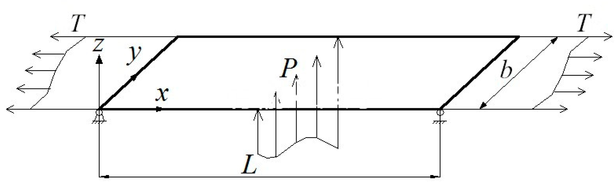
2.1. The Establishment of the Simulation Model

Figure 1 shows a schematic diagram of the SI-FLAT flatness meter measurement platform in a certain 2180 mm tandem cold rolling production line. The middle part of the platform is an airflow channel, and the lower part is connected with an air pump and an air conditioner by pipelines. The eddy current ranging sensor is used for measuring the thin strip amplitude: Its best detection distance range is from 0.1 to 0.2 mm, the rated flow of the fan is 125 m3/min, the detection length of the flatness meter is 1000 mm, and the maximum strip width is 2100 mm.
A related study [9] showed that the strip speed had little effect on the natural frequency of the thin plate, so the influence of speed was not considered in this paper, and the simulation model was simplified as follows:
  • The strip constraints were simplified into two sides with support and two sides without support;
  • The strip and the measurement platform were set as solid wall boundary conditions;
  • The exit pressure of the fluid domain was set as atmospheric pressure;
  • The airflow channel was simplified into a rectangle, which had the same area as the total stomata and the same length as the airflow channel, and the width of the rectangle was calculated as 15.73 mm based on the actual dimensions.
Figure 2 shows a schematic diagram of the strip dynamic model, in which L is the detection length; b is the strip width; T is the tension applied in the strip rolling direction; and P is the airflow excitation load, which is imposed on the fluid–structure interaction interface through the airflow channel.
According to the data in Figure 1 and Figure 2, a simulation geometric model was established by UG (Unigraphics NX 12.0, Siemens PLM Software, Plano, TX, USA). A front view, bottom view, and three-dimensional view of the model are respectively shown in Figure 3a–c, in which h is the strip thickness and c is the distance between the lower surface of the strip and the detection platform. The strip was a single metal material with the elastic modulus E of 210 GPa. The Poisson ratio μ was 0.3, and the density ρ was 7850 kg/m3. In the grid generation of the strip, when the grid size was larger than 0.03 mm, there were big deviations in the calculation results of the amplitude, and the model exhibited a poor convergence. When the grid size was 0.01 or 0.02 mm, the difference between the two amplitude calculation results could be neglected, and furthermore, the calculation time of 0.02 mm was much shorter than that of 0.01 mm. Thus, after comprehensive consideration, the strip was meshed in hexahedral grids with a size of 0.02 mm. Moreover, the strip constraints were simplified into two sides with support and two sides without support. The tension was imposed on the simply supported side, and the flatness stress was imposed on each node of the strip.
The fluid module used the ideal air module in CFX (ANSYS CFX, ANSYS Inc., Canonsburg, PA, USA). The alternating aerodynamic load was imposed on the inlet of fluid, and the atmospheric pressure in the outlet of the fluid was set as the standard atmospheric pressure. Moreover, the grid size of the fluid in the contact area above and under the strip was the same as that of the strip. This was mainly because in the case of dynamic mesh technology, the larger the deviation between the grid size of the fluid above and under the strip and that of the strip, the worse the convergence. In addition, the grid size of the other fluid had little effect on the convergence of the model, so automatic grid generation in the ANSYS Workbench (ANSYS Workbench 17.0, ANSYS Inc., Canonsburg, PA, USA) was used, considering the time cost.
Obviously, the fluid–structure interaction was generated by the interaction of the fluid and the solid, and its analysis included an unsteady calculation of flow field and a transient dynamic calculation of structure. In this paper, the characteristics of fluid–structure interaction in the thin strip under different streams (i.e., alternating aerodynamic loads) were simulated in a large space. The strip vibration calculation used the transient dynamics method in ANSYS, the control equation used the unsteady Reynolds average Navier–Stokes equation, the space used a second-order upwind scheme, the time used the second-order Euler backward-difference scheme, the coupling calculation used dynamic mesh technology, and the turbulence model selected a k-ε model [10,11].
The same physical time step was used in the transient dynamic calculation of structure as well as the unsteady calculation of flow field. According to the frequency of aerodynamic load during the analysis, each pulsation period was 0.1–0.2 s, and the calculation time was set to 0.8 s. Thus, the time step was set to 0.01 s, and this time step could guarantee calculation accuracy and efficiency at the same time. In each physical time step, a sequential solution was adopted: That is, at first the three-dimensional transient flow field was solved, and then the transient dynamic characteristics of structure were analyzed.
By setting a consistent fluid–structure interaction interface and reasonably simplifying the boundary conditions, the model was stably convergent and the calculation time of each simulation condition was about 50 min.

2.2. The Design of the Simulation Conditions

The factors that affect strip amplitude distribution include the strip thickness, strip width, aerodynamic load, tension, flatness defects, etc. The specific width and thickness were chosen according to the actual production to analyze the influences of other factors, and the main influencing factors are shown in Table 1, in which the aerodynamic load P is pulsating load, and a and ω are pulsating load variable parameters.
Typical cold rolling flatness generally includes no wave, the center wave, the double-edge wave, the edge-center composite wave, and the quarter wave [12]. In the actual production, through observation of a large number of the whole coils of strips, it could be found that a coil of strip had a certain flatness change in its full length, but with a short length, it could be considered that the flatness of the strip did not change. Based on a measurement of the SI-FLAT flatness meter in this paper, the measured strip length was 1 m, and this could be treated as the strip flatness approximately not changing.
According to the Saint-Venant principle, the method of applying uneven tensions in the strip length direction cannot truly express the flatness with uneven distributions of the internal tensile stress. Therefore, an uneven temperature was imposed on the strip in this paper, and the desired flatness internal tensile stress was obtained through a thermodynamic analysis of the finite element software. Table 2 shows the expressions of applied uneven temperature [13], where x is the normalized strip width, x [ 1 , 1 ] , and y is the temperature at x. By setting k1 = −24, k2 = 10.8, a comprehensive flatness of 4.5 I could be obtained.
The deviation, which is the difference between the flatness set by the finite element model and the flatness calculated from the amplitude calculation results by the finite element model, is defined as the flatness calculation deviation, and the calculation steps are shown as follows:
(1) An uneven temperature was imposed on the strip, and the internal tensile stress of the strip was calculated by the thermal stress module in ANSYS. Then, the setting flatness using the tensile stress difference method was
ρ 1 ( i ) = 1 μ 2 E ( σ ( i ) σ ¯ ) ,
where ρ 1 ( i ) is the setting flatness using the tensile stress difference method, σ ( i ) is the stress value of the ith measurement area in the strip, σ ¯ is the strip average tensile stress, E is the strip elastic modulus, and μ is the strip Poisson ratio;
(2) The strip amplitude was calculated by the fluid–structure interaction finite element model simulation, and the calculation flatness was obtained by the flatness calculation model of the SI-FLAT flatness meter,
ρ 2 ( i ) = σ ¯ E × { 1 A ( i ) ( 1 A ¯ ) ( 1 A ¯ ) } ,
where ρ 2 ( i ) is the calculation flatness of the simulation results, A ( i ) is the forced vibration amplitude in the ith measurement area of the strip, and ( 1 A ¯ ) is the average value of amplitude reciprocals in each measurement area of the strip;
(3) The setting flatness using the tensile stress difference method was subtracted from the calculation flatness of the simulation results, and the flatness calculation deviation δ could be obtained:
δ = ρ 2 ( i ) ρ 1 ( i ) .

3. Numerical Simulation Results and Analysis

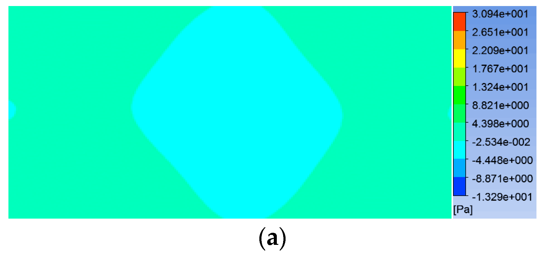
3.1. The Influences of Fluid–Structure Interaction on Strip Amplitude Distribution and Flatness Calculation Deviation

On the one hand, the flatness deviation of the strip was analyzed while ignoring the interaction between the fibrous bundles, and the airflow excitation force was simplified into being the force that directly acted on the strip (called without interaction) [5]. On the other hand, based on the actual situation, the strip and the airflow excitation were in a bidirectional fluid–structure interaction through CFX (called with interaction).
Figure 4 shows the strip amplitude distribution with or without interaction when the strip thickness was 0.8 mm, the width was 1600 mm, the tension was 30 MPa, the injection speed was 1 + sin ( 18 π t ) m/s, and the strip had no flatness defects. It can be seen that the amplitude distributions were obviously different under the two conditions. The two amplitude distributions were both less changed, and the amplitudes were relatively close within 350 mm from the strip midpoint. The closer they were to the edge, the larger the amplitude distribution change and the larger the difference in the two amplitudes. Moreover, the amplitude distribution forms changed oppositely, and the two amplitudes had the biggest difference within 200 mm from the edge.
Putting the strip amplitude from Figure 4 into Equation (2), the strip calculation flatness under the SI-FLAT flatness calculation model could be calculated. As shown in Figure 5, it can be seen that the two strips without initial flatness defects both exhibited uneven flatness, indicating that the calculation results of Equation (2) were biased. At the same time, the flatness forms with or without interactions were obviously different, especially in the case of bidirectional interaction between the strip and the airflow: The strip flatness in the middle was small and uniform, while the flatness on the edge had the biggest difference, exceeding 20 I. On the one hand, the simulation results show the importance of considering the bidirectional fluid–structure interaction: It could be found that the strip flatness distribution with interaction was similar and antisymmetric to the real flatness target curve used in the field (as shown in Figure 6). Thus, the results with interaction were more suitable to the actual situation. The following analyses and calculations only consider interactions. On the other hand, the 20 I did not match the real flatness target curve, which also shows that the flatness calculation deviation must be considered. Therefore, the flatness calculation deviations under different conditions were subsequently analyzed, which provided a theoretical basis for correcting the measurement results of the flatness meter.
Figure 7 shows the pressure cloud picture above and under the strip at a certain time with interaction. It can be clearly seen that the middle position under the strip was the contact area between the airflow and the strip, and the pressure in the contact area showed a uniform distribution in the middle and a gradual decrease on the edge. At the same time, the pressure above the strip was negative in partial middle areas as well as in small areas on the edge, while the pressure in other areas was positive. However, all of the values were very small. The basic reason for the strip vibration was that the pressure difference was different above and under the strip, and which made the amplitude distribute uniformly in the middle and decrease rapidly on the edge was that: In the measurement position, the pressure difference was uniformly distributed along the upper and lower sides of the middle strip, while it decreased along the upper and lower sides of the edge. The edge pressure was especially significantly different from the middle pressure.

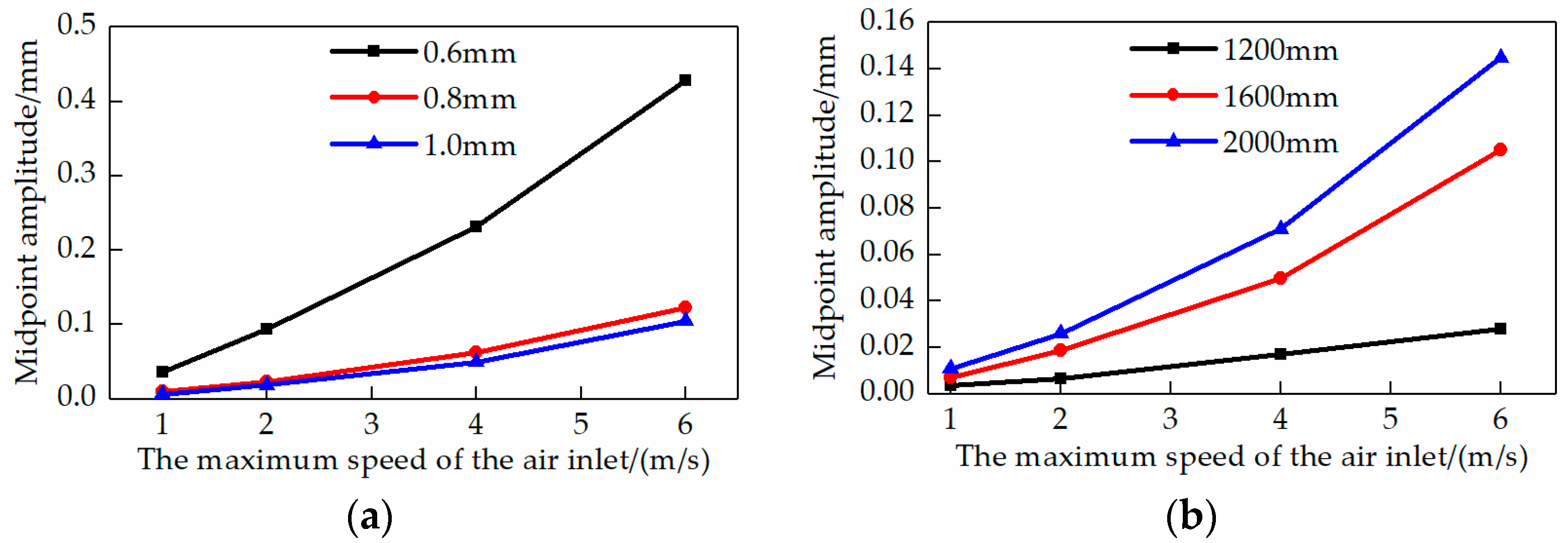
3.2. The Influences of Different Aerodynamic Loads on Strip Midpoint Amplitude and Flatness Calculation Deviation

In actual situations in the field, in order to make the strip amplitude within the optimal measurement range of the sensor, the most commonly used and most important method for adjusting the strip amplitude is to change the speed of the air inlet of the SI-FLAT flatness meter. Thus, first, the influence of different aerodynamic loads on the strip midpoint amplitudes was simulated, which provided a reference for setting the excitation force in the field.
The rated flow of the fan in the SI-FLAT flatness meter was 125 m3/min, and the conversion between the fluid flow and the flow speed is shown in Equation (4):
Q = v × A ,
where Q is the fluid flow, v is the flow speed, and A is the sectional area of the airflow channel.
The rated flow speed of the fan was calculated at 64m/s based on Equation (4), and the actual flow speed was far less than the rated flow speed according to the field data. In the fan speed range that was actually used in field, the midpoint amplitude changes of different thicknesses under different alternating aerodynamic loads (namely the different maximum speeds of the air let) were separately calculated when the width was 2000 mm and the other parameters were unchanged, as shown in Figure 8a. At the same time, the midpoint amplitude changes of different widths under different maximum speeds of the air let were also separately calculated when the thickness was 1 mm and the other parameters were unchanged, as shown in Figure 8b.
Figure 8 shows that, under the same conditions, the thicker the strip, the smaller the amplitude, and the wider the strip, the bigger the amplitude. The reason was that with the strip thickness increasing, the moment of inertia increased and the deflection decreased. With the strip width increasing, the effect between the vertical fibrous bundles decreased and the amplitude increased. Therefore, the size of the alternating aerodynamic load (i.e., changes in the speed of the air let) had a significant influence on the amplitude, so this was an effective amplitude adjustment method.
From Figure 8, it can also be seen that when the strip was microamplitude-vibrated, with the airflow speed increasing, the midpoint displacements of different strip widths and thicknesses increased in the form of a quadratic polynomial, and the determination coefficients R 2 of the fitted quadratic curves were all above 0.99. This was because the alternating aerodynamic loads acted on the lower surface of the strip in the form of wind speed in the airflow channel, and the strip was simplified into the vertical fibrous bundles which did not affect each other, according to the basic theory of material mechanics. In the range of microamplitude vibrations, the excitation force on the fibrous bundles was proportional to the strip deflection, and the excitation force was proportional to the square of the airflow speed, so the displacement of the vibration point increased with the airflow speed in the form of a quadratic polynomial.
Based on an analysis of the influence of different aerodynamic loads on the strip midpoint amplitude, the influence of different aerodynamic loads on the flatness calculation deviation in the width direction was further analyzed. The flatness calculation deviations of the no-defect strip were calculated when a took different values, which was within the aerodynamic loads a + a sin ( ω t ) , as shown in Figure 9. It can be seen that the flatness calculation deviations of the no-defect strip were almost equal under different airflow excitation speeds, which presented a phenomenon similar to Figure 5, where the flatness deviations in the middle strip approached 0 and those on the edge rapidly increased.

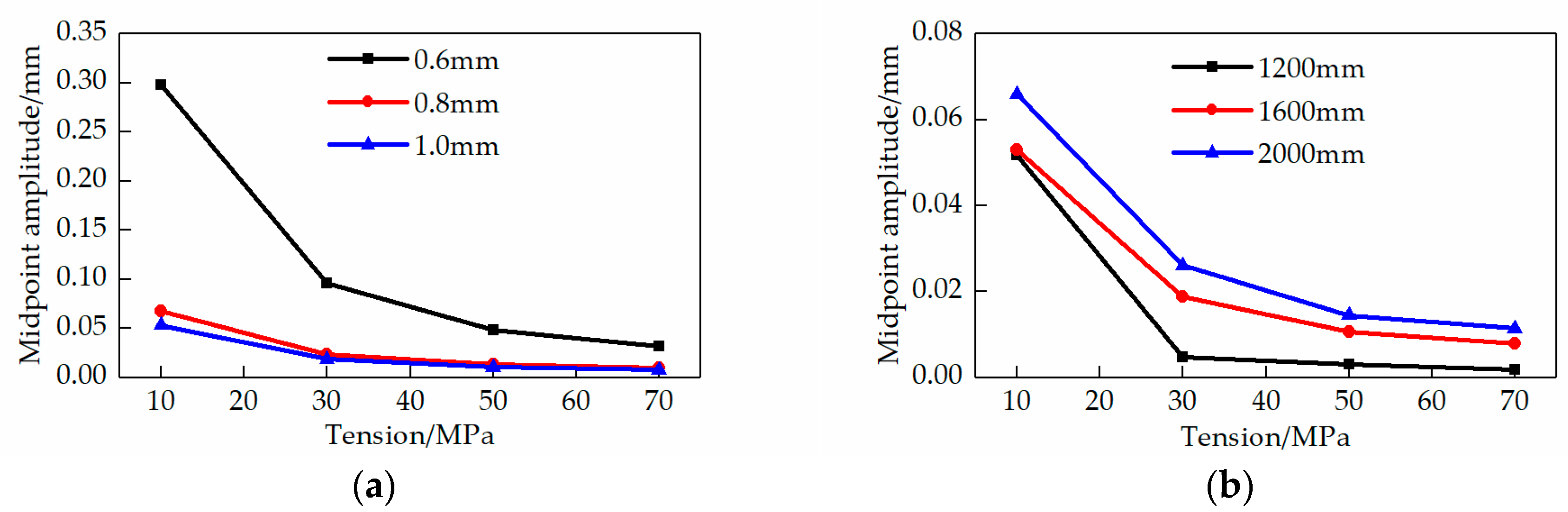
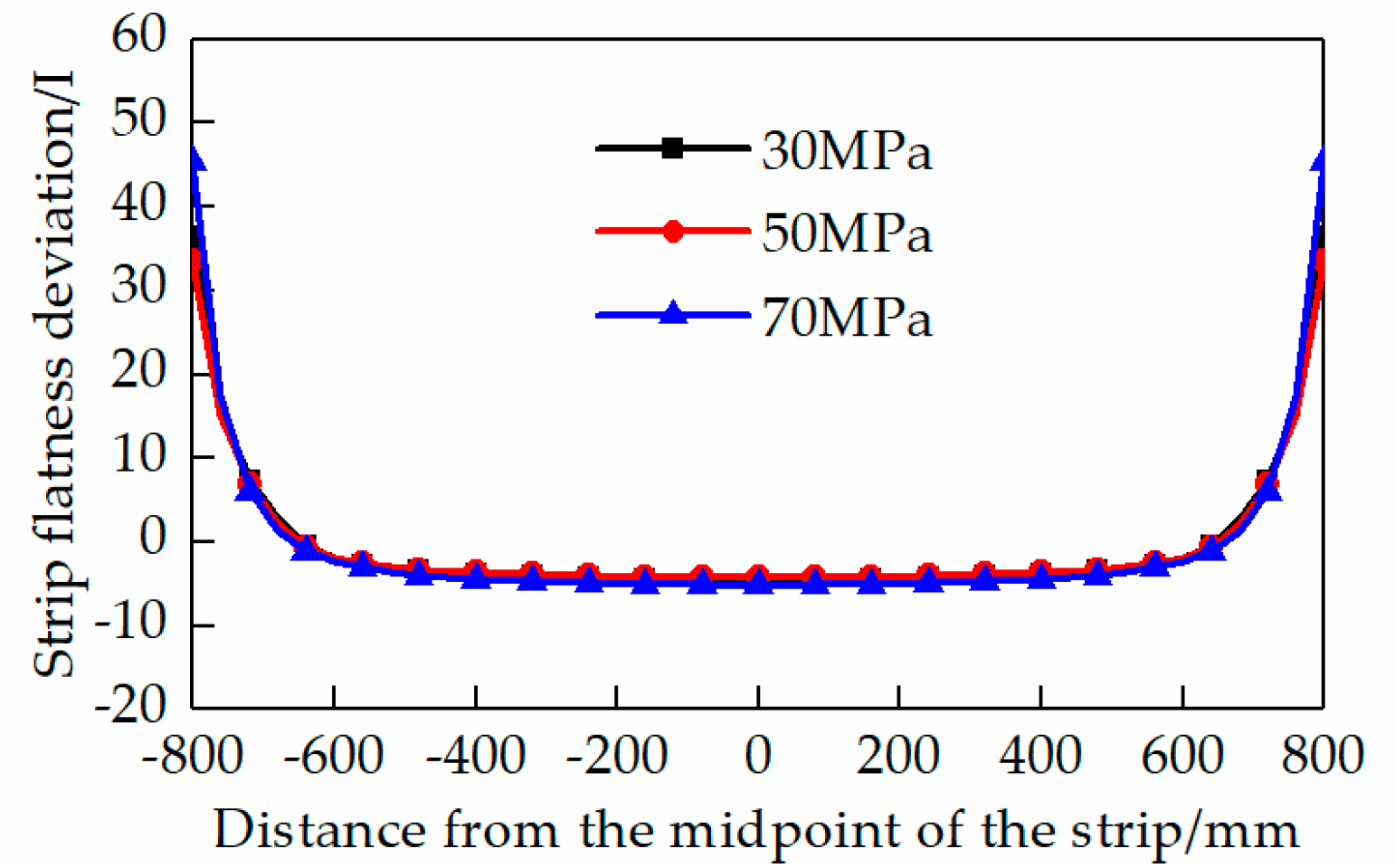
3.3. The Influences of Different Tensions on Strip Midpoint Amplitude and Flatness Calculation Deviation

The SI-FLAT flatness meter detected when the strip was under large tension and maintained no dominant waves [14]. The change in tension not only affected the online buckling, but also directly affected the strip amplitude under the aerodynamic loads.
The midpoint amplitude changes of different thicknesses under different tensions were separately calculated when the width was 2000 mm and other parameters were unchanged, as shown in Figure 10a. At the same time, the midpoint amplitude changes of different widths under different tensions were also separately calculated when the thickness was 1 mm and other parameters were unchanged, as shown in Figure 10b.
It can be seen from Figure 10 that, under the same conditions, the thicker the strip, the smaller the amplitude. However, the larger the strip thickness was, the less obvious the influence of thickness changes on the amplitude were. Midpoint displacements of 0.8 mm and 1 mm in thickness were almost equal in the case of increased tensions. The wider the strip, the larger the amplitude, but with the strip width increasing, the midpoint displacement decreased more slowly.
The influence of changes in tension on the strip amplitude was significant, so changing the tension during detection was also a direct and effective amplitude adjustment method. In the range of microamplitude vibrations, when the tension increased, the displacement of the vibration point decreased exponentially, and the determination coefficients R 2 of the fitted exponential curves were all above 0.99. However, the displacement of the vibration point did not change obviously when the tension was greater than 40 Mpa. In order to achieve the best detection range of the flatness meter, it was necessary to properly adjust the speed of the air inlet.
Figure 11 shows the influence of different tensions on the flatness calculation deviation in the strip width direction. It can be seen that the flatness calculation deviations of the no-defect strip under different tensions presented a similar conclusion to the flatness calculation deviations under different aerodynamic loads.

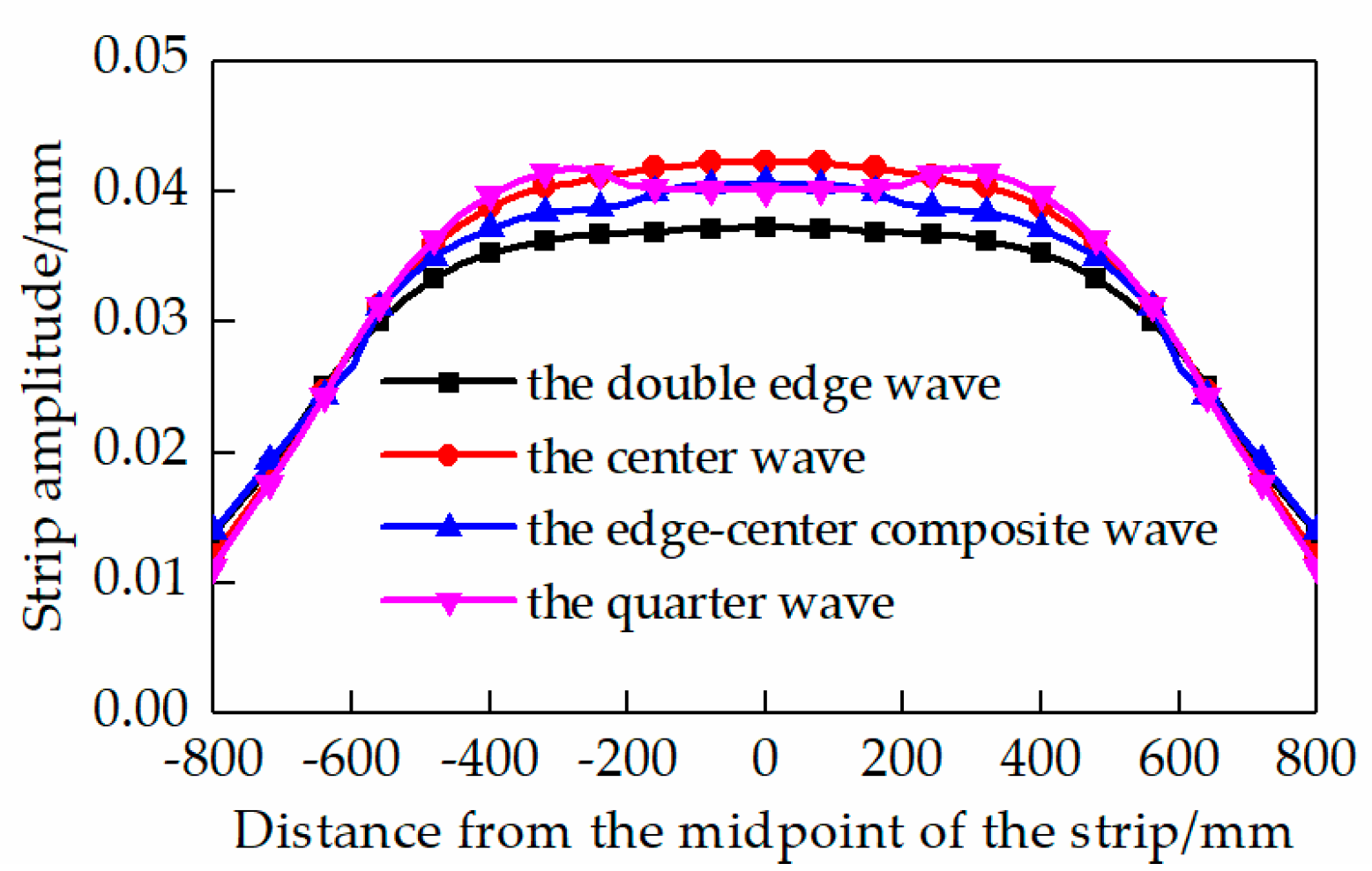
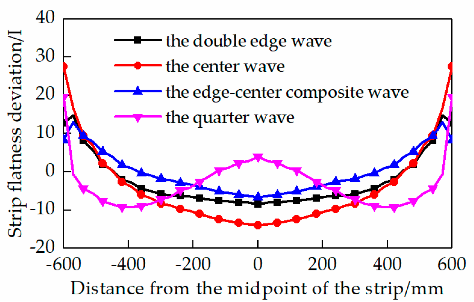
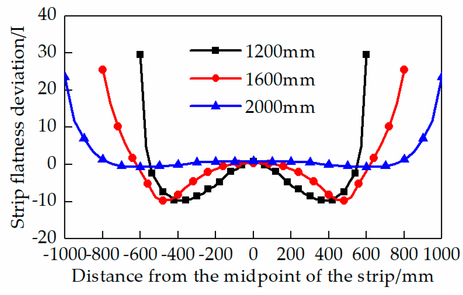
3.4. The Influences of Different Flatness Defects on Strip Amplitude Distribution and Flatness Calculation Deviation

Different flatness defects reflect the characteristics of the strip width direction and have a direct effect on the strip amplitude distribution. Thus, the characteristics of the strip amplitude distributions of the four typical flatness defects as well as the influence of these flatness defects on the flatness calculation deviation are concretely analyzed in this section.
The amplitude distributions along the strip width were calculated when the flatness defects were expressed as the double-edge wave, the center wave, the edge-center composite wave, and the quarter wave. At the same time, the strip width was 1600 mm, the thickness was 0.8 mm, the tension was 25 MPa, the aerodynamic load was 1 + sin ( 18 π t ) m/s, and the flatness value was 4.5 I, as shown in Figure 12.
In Figure 12, first, it can be seen that the amplitudes of all of the waves were large in the middle and decreased along the edge because of the uneven distribution of the excitation force. Second, the amplitude distribution forms along the strip width were different under different waves, concretely shown as follows: Under the double-edge wave and the center wave, the amplitudes in the middle were distributed uniformly, but the difference was large and reached 9.6 μm at its maximum, and the amplitudes on the edge were sharply reduced. The amplitudes on the edge under the double-edge wave and the edge-center composite wave were slightly larger than those under the center wave and the quarter wave, and the maximum difference was 1.7 μm. The amplitude distribution of the edge-center composite wave was appreciably salient in the middle of the strip, and the amplitude on the edge was basically the same as that of the double-edge wave. The amplitude of the quarter wave significantly increased at a quarter distance from the edge. It was considered that, in the case of tension, the compressive stresses of different waves were all offset, so the compressive stress at the original site was about 1 MPa, and the tensile stress increased to about 40 MPa. Meanwhile, the strip was simplified into fibrous bundles that could affect each other along the width, and the fibrous bundles were simplified into Euler beams that were simply supported and pulled at both sides. According to the Euler beam model, the greater the tension is, the smaller the deflection of the beam is. Thus, for the center wave in the middle of the strip, the amplitudes in the areas with waves had a significant increase compared to those in the areas without waves.
Figure 13 shows the flatness deviations of different flatness defects. It can be seen that under different flatness defects, the forms of the flatness deviation changed greatly compared to those of the amplitude. In general, the deviations in the edge were large, and the deviation forms were similar under the double-edge wave, the center wave, and the edge-center composite wave. At the same time, the fluctuation characteristics of the deviations were opposite to the initial flatness deviations, such as with the center wave. It was shown that the double-edge wave occurred in the areas without waves on the edge, and the amplitude decreased in the areas with waves in the middle.
From Figure 12 and Figure 13, it can be seen that the amplitude distribution and the flatness calculation deviation of the quarter wave were the most complicated in the four flatness defects. Therefore, the variation laws of the amplitude and the corresponding calculation deviation of the quarter wave under different conditions should be emphatically analyzed.
Figure 14 shows the amplitude distributions of the strips with the quarter wave of different widths. It can be seen that there was a big difference in the amplitude changes of different widths, concretely shown as follows: When the width increased, the amplitude increased significantly, but the amplitude fluctuation became more and more complicated. Meanwhile, the amplitude in the middle was less than that of a quarter distance from the edge when the strip width was 2000 mm.
Figure 15 shows the corresponding flatness calculation deviations. It can be seen that, when the width decreased, the flatness calculation deviation increased and the change was more violent. The reason was that, with the width decreasing, the strip alternated more violently in the areas with or without waves within the unit width.
Figure 16 shows the amplitude distributions of the strips in different thicknesses with the quarter wave. It can be seen that, when the thickness increased, the amplitude on the edge was almost unchanged, while the amplitude in the middle decreased significantly.
Figure 17 shows the flatness calculation deviations of different thicknesses. It can be seen that the distribution forms of the calculation deviation were similar under different thicknesses: However, when the thickness increased, the calculation deviation increased.
In summary, the strip amplitude distribution and the flatness calculation deviation were different under different initial flatness defects, and for the same flatness defect, the width and the thickness also had great influence on the amplitude distribution and the flatness calculation deviation. Thus, these factors should be considered in the correction of the flatness calculation deviation and the optimization of the target curve.

4. Conclusions

First, the amplitudes of the strip were significantly different with or without interaction, and the amplitude with interaction was more suitable for the actual measurement of the flatness meter. Moreover, in the situation of an interaction, the amplitude distributed uniformly in the middle and decreased rapidly on the edge, which indicated that the detection results should be corrected and compensated. In addition, the simulation results also had a corresponding relation with the target curve, which was used for flatness correction in the field.
Second, the variation laws of the strip midpoint amplitude under different factors were analyzed. This showed that with the alternating aerodynamic load increasing, the midpoint amplitude increased in the form of a quadratic polynomial. However, with the tension decreasing, the midpoint amplitude decreased exponentially. Thus, the results also provide a theoretical basis for reasonably setting the working distance of eddy current sensors.
Finally, the strip amplitude distribution and the flatness calculation deviation under different initial flatness defects were analyzed. This showed that the fluctuation characteristics of the deviation were opposite to the initial flatness deviation. For example, the most complicated quarter wave was deeply analyzed: It could be seen that with the width decreasing or the thickness increasing, the flatness calculation deviation increased and changed more rapidly. Thus, the dimensions of a strip should be considered in the actual flatness calculation deviation correction and the target curve design.

Author Contributions

H.L. led the research work and the writing of the article; G.H. wrote the paper; J.Y. did the FEM analysis; N.L. and J.Z. participated in the discussion of the research.

Funding

This work was supported by “the National Key Technology R&D Program of the 12th Five-year Plan of China” (grant no. 2015BAF30B01) and “the Fundamental Research Funds For the central Universities” (grant no. FRF-BR-16-025A, FRF-TP-15-016A3).

Acknowledgments

The authors thank Wuhan Iron & Steel (Group) Company for the industrial data support.

Conflicts of Interest

The authors declare no conflicts of interest.

References

  1. Li, H.B.; Bao, R.R.; Zhang, J.; Jia, S.H.; Chu, Y.G.; Liu, H.C. Cluster analysis of strip flatness characteristics for ultra-wide cold rolling mills. J. Univ. Sci. Technol. B 2016, 11, 1569–1575. [Google Scholar] [CrossRef]
  2. Yang, G.H.; Zhang, J.; Cao, J.G.; Yan, Q.T.; Chen, X.H.; Jia, S.H. Strip non-contact flatness detection principle and its detection system. Metall. Ind. Autom. 2009, 33, 665–668. [Google Scholar]
  3. Spreitzhofer, G.; Duemmler, A.; Riess, M.; Tomasic, M. SI-FLAT contactless flatness measurement for cold rolling mills and processing lines. Rev. Métall. 2012, 102, 589–594. [Google Scholar] [CrossRef]
  4. Qin, Z. Application of a new cold rolling strip type SI-FLAT in cold tandem mill. Metall. Ind. Autom. 2004, 28, 63–65. [Google Scholar] [CrossRef]
  5. Yang, G.H.; Zhang, J.; Cao, J.G.; Li, H.B.; Huang, Q.B. Relationship between strip amplitude and shape for shapometer based on airflow excitation and eddy current. J. B Inst. Technol. 2015, 35, 671–676. [Google Scholar] [CrossRef]
  6. Li, N.; Kong, N.; Li, H.B.; Zhang, J.; Jia, S.H.; Chu, Y.G.; Liu, H.J. Analysis of fluid-structure interaction vibration based on the detection principle of SI-FLAT flatness measurement systems. J. Univ. Sci. Technol. B 2017, 39, 593–603. [Google Scholar] [CrossRef]
  7. Hu, S.L.; Lu, C.J.; He, Y.S. Numerical analysis of fluid-structure interaction vibration for plate. J. Shanghai Jiaotong Univ. 2013, 47, 1487–1493. [Google Scholar]
  8. Lu, K.; Zhang, D.; Xie, Y.H. Fluid-structure interaction for thin plate with different flow parameters. Proc. Chin. Soc. Electr. Eng. 2011, 31, 76–82. [Google Scholar]
  9. Li, J.; Yan, Y.H.; Guo, X.H.; Wang, Y.Q.; Wei, Y. On-line control of strip surface quality for a continuous hot-dip galvanizing line based on inherent property of thin plate. Chin. J. Mech. Eng. 2011, 47, 60–65. [Google Scholar] [CrossRef]
  10. Zhang, J.P.; Guo, L.; Wu, H.L.; Zhou, A.X.; Hu, D.M.; Ren, J.X. The influence of wind shear on vibration of geometrically nonlinear wind turbine blade under fluid–structure interaction. Ocean. Eng. 2014, 84, 14–19. [Google Scholar] [CrossRef]
  11. Xie, L.; Zhao, X.; Zhang, J. ANSYS CFX Fluid Analysis and Simulation; Electronic Industry Press: Beijing, China, 2012. [Google Scholar]
  12. Yang, G.H.; Zhang, J.; Li, H.B. Transverse distribution law of airflow excitation force for SI-FLAT contactless shapometer. Comput. Aided Draft. Des. Manuf. 2016, 26, 41–47. [Google Scholar]
  13. Bao, R.R. Characteristic Analysis and Control of Complex Strip Flatness in Ultra-wide Cold Strip Mill. Ph.D. Thesis, University of Science and Technology Beijing, Being, China, 2015. [Google Scholar]
  14. Li, N. Study on the Cold Rolled Strip Buckling and Vibration Based on Incompatible Deformation Theory. Ph.D. Thesis, University of Science and Technology Beijing, Being, China, 2017. [Google Scholar]
Figure 1. A schematic diagram of the SI-FLAT flatness meter measurement platform.
Metals 09 00496 g001
Figure 2. A schematic diagram of the strip dynamic model.
Metals 09 00496 g002
Figure 3. Flow field model diagram: (a) front view; (b) bottom view; (c) three-dimensional view.
Metals 09 00496 g003
Figure 4. Strip amplitude distribution with or without fluid–structure interaction.
Metals 09 00496 g004
Figure 5. Strip flatness distribution with or without fluid–structure interaction.
Metals 09 00496 g005
Figure 6. Strip flatness target curve.
Metals 09 00496 g006
Figure 7. Strip pressure distribution above and under the strip. (a) Above the strip; (b) under the strip.
Metals 09 00496 g007aMetals 09 00496 g007b
Figure 8. The midpoint amplitude changes of different strips with maximum speeds of the air inlet. (a) Different thicknesses; (b) different widths.
Metals 09 00496 g008
Figure 9. The effect of airflow excitation speed on the flatness calculation deviation.
Metals 09 00496 g009
Figure 10. The midpoint amplitude changes of different strips with tensions. (a) Different thicknesses; (b) different widths.
Metals 09 00496 g010
Figure 11. The effect of tensions on the flatness calculation deviation.
Metals 09 00496 g011
Figure 12. The strip amplitude distribution of different flatness defects.
Metals 09 00496 g012
Figure 13. The effect of different flatness defects on the flatness calculation deviation.
Metals 09 00496 g013
Figure 14. Amplitude distribution of different widths.
Metals 09 00496 g014
Figure 15. The effect of different widths on the flatness calculation deviation.
Metals 09 00496 g015
Figure 16. Amplitude distribution of different thicknesses.
Metals 09 00496 g016
Figure 17. The effect of different thicknesses on the flatness calculation deviation.
Metals 09 00496 g017
Table 1. Conditions under different combinations of factors.
Influencing FactorsValues
Width b mm1200, 1600, 2000
Thickness h mm0.6, 0.8, 1
Aerodynamic load P m/s a + a sin ( ω t )
Tension T MPa30, 50, 70
Flatness formsno wave, the center wave, the double-edge wave, the edge-center composite wave, the quarter wave
Table 2. Expressions of uneven temperature.
Flatness DefectsExpressions
The center wave y = k 1 2 ( 3 x 2 1 )
The double-edge wave y = k 2 2 ( 3 x 2 1 )
The edge-center composite wave y = k 2 8 ( 35 x 4 30 x 2 + 3 )
The quarter wave y = k 1 8 ( 35 x 4 30 x 2 + 3 )

