Article

Computer-Integrated Platform for Automatic, Flexible, and Optimal Multivariable Design of a Hot Strip Rolling Technology Using Advanced Multiphase Steels

1
Department of Applied Computer Science and Modelling, AGH University of Science and Technology, al. Mickiewicza 30, 30-059 Kraków, Poland
2
Institute for Ferrous Metallurgy, ul. K. Miarki 12, 44-100 Gliwice, Poland
3
CEIT, Paseo de Manuel Lardizabal 15, 20018 Donostia-San Sebastián, Spain
4
ArcelorMittal Maizières Research SA, Voie Romaine, 57280 Maizières-lès-Metz, France
5
Department of Computer Science, AGH University of Science and Technology, al. Mickiewicza 30, 30-059 Kraków, Poland
*
Author to whom correspondence should be addressed.
Metals 2019, 9(7), 737; https://doi.org/10.3390/met9070737
Submission received: 1 May 2019 / Revised: 5 June 2019 / Accepted: 19 June 2019 / Published: 29 June 2019
(This article belongs to the Special Issue Researches and Simulations in Steel Rolling)

Abstract

:
The paper presents the design and implementation of a computer system dedicated to the optimization of a hot strip rolling process. The software system proposed here involves the flexible integration of virtual models of various devices used in the process: furnace, descalers, rolling stands, accelerated cooling systems, and coiler. The user can configure an arbitrary sequence of operations and perform simulations for this sequence. The main idea of the system and its implementation details are described in the paper. Besides the computer science part, the material models describing the rolling parameters, microstructure evolution, phase transformations, and product properties are also presented. Effect of precipitation was accounted for various stages of the rolling cycle. Experimental tests were performed to generate data for identification of the models. These include plastometric tests, two-step compression tests, and dilatometric tests. Following this, physical simulations of rolling cycles were performed on Gleeble 3800 to supply data for the verification and validation of the models. Finally, case studies of modern industrial processes were performed, and the selected results are presented.

1. Introduction

Studying the rolling-related processes by building a digital twin of the hot rolling mill can be described as a multistep workflow involving [1]:
  • Design of a virtual hot rolling mill;
  • Simulation of the rolling process with the parameter study approach;
  • Output data exploration with sensitivity analysis (SA) methods to discover relationships between the rolling mill parameters and the thermo-mechanical properties of the final product.
Each of these steps has different requirements regarding easiness of use, computing power, and process monitoring. Designing and developing of a system supporting this multistep workflow is the main objective of the whole project. Problem of the computer-aided design of the hot strip rolling technology has been in the field of interest of researchers for more than a half-century. The first fundamental works in this field were focused on the development of a thermo-mechanically controlled process (TMCP), which required the development of both metallurgical [2,3] and numerical models [4,5]. Following the development of the computing power, microstructure evolution models were implemented in the finite element (FE) codes, and fully coupled thermal-mechanical-metallurgical simulations became possible [6]. In late 1990s and at the beginning of this century, several detailed process models describing the whole manufacturing cycle were developed [7,8].
The first models developed a half-century ago had serious limitations when applied under conditions different from those under which they were developed (short interpass times, privilege recovery over recrystallization). Current models became more reliable and accurate. The steel industry, nowadays, needs to develop AHSS (Advanced High Strength Steel) grades [9] in a cost-effective way and get them to the market at the earliest, while manufacturing them within the constraints of their mill configuration. This needs progress in terms of modelling performed, i.e., by allowing effective modelling of new tendencies such as, the low coiling temperatures required for hot rolled dual phase (DP) steel. The mentioned model limitations justify the creation of a computer system dedicated to flexible designing and modelling of hot rolling technology. Some of the systems based on hot rolling metallurgical models have been developed and used for defining thermo-mechanical cycles or monitoring mechanical properties. Worldwide experiences are reported in the literature [10,11]. Software packages such as TK-StripCam by ThyssenKrupp Stahl [10], MetModel by Corus [12], MicroStructureMonitor by Siemens [13], VAI-Q strip [11] by Voestalpine and Industrieanlagenbau (VAI), and HSMM [14] by the INTEG process group are available. The system Slimmer commonly used in the industry is described in [4,15]. The authors’ model was applied in [16] for simulation of hot DP strip rolling. All these packages are based on a direct approach. They are not integrated with data/knowledge bases and inverse solutions based on the optimization techniques.
Review of the literature shows that currently available systems accurately predict the deformation behavior for only typical rolling routes. New tendencies in development of rolling strategies, such as high austenite deformations near two-phase region or bainite/martensite evolution in coils, are still a challenge. Thus, over the past few years, more attention has been paid to the models that can predict the microstructural evolution during hot rolling, subsequent cooling and coiling, followed by the prediction of mechanical properties in the room temperature. The goal is usually to predict the microstructure of the materials and to optimize the process conditions to obtain the best combination of strength, ductility, and weldability in the as-rolled product. The computer system VirtRoll, which was originally developed at the AGH University of Science and Technology [17], was further extended within the RFCS (Research Fund for Coal and Steel) project [18], where it was applied to design optimal manufacturing strategies. Description of the upgraded hybrid version of the VirtRoll and showing its capabilities to face all challenges occurring during technology design for new generation multiphase steels is one of the objectives of the present paper. Results of case studies for bainitic and HSLA (High Strength Low Alloyed) steels, as well as for new generation AHSSs, are presented. Testing VirtRoll capability to design routes by taking advantage from the effect of precipitation is the final objective.

2. VirtRoll Hybrid Computer System

The VirtRoll system, which was developed by the Authors within the project [18], combines models, data and knowledge bases, and the inverse approach to design optimal hot strip rolling processes. It allows the design of rolling line composed of basic equipments like furnace, descalers, rolling stands, laminar cooling, ultra-fast cooling devices, coilers, etc. Depending on the selected materials, specific numerical models (see Section 4) can be implemented in the system. The main implementation procedure is based on the workflow idea and is supported by software framework for workflow design, creation, and performance. This approach was integrated with the steel modelling workbench, which is an open software environment, where various models can be linked and run to allow the modular development of integrated model at various stages of the manufacturing. The integration was based on the common data flow model. An overview of the system along with main steps of the workflow is depicted in Figure 1.

2.1. Methodology

The first step of the workflow allows to design a virtual representation of the hot rolling mill including selection of devices, their location, and configuration parameters. The VirtRoll system supports this step by providing a virtual workplace with a graphical drag and drop editor of the rolling mill and a toolbox of available configurable devices. The user can select a project already stored in the system database or prepare a new mill design. Moreover, the user can save the work at any given moment and return to it in the future. The second step is the numerical simulation of the rolling process in a parameter study manner. The user prepares a space with parameters including the material description, configuration of devices, and process variables. Briefly, the parameter study includes:
  • Computational tasks scheduling to high performance computational infrastructures;
  • On-line progress monitoring of the simulations with capability to adjust computing power or extend the parameter study interactively;
  • Collecting simulation results and further analysis.
These functionalities are attained by integrating the VirtRoll system with the Scalarm platform described in [19] and extending it where required.
The third step of the workflow is exploration of the results obtained from simulations. The main objective is to reach a better understanding of the analyzed process and discover advantages and disadvantages of the designed virtual mill regarding final properties of the product. The conducted parameter study provides sufficient data to perform a complete sensitivity analysis and to discover relationship between the setup and results.

2.2. Technology of the System Design

The technology used in this paper is based on three main elements: the graphical user interface (GUI) of the VirtRoll system, the middleware in form of the Scalarm platform, as well as the numerical simulations of the rolling/cooling processes. The GUI created as a web-based module facilitates access from different operating systems and devices. Application of modern web technologies, e.g., AJAX and HTML5, fulfills requirements regarding various operating systems, interactivity, and easiness of use. Information about materials and devices available for the rolling mill designers is stored in the database, see [1] for details. In contrast to web-based high-level solutions, the VirtRoll computing module, used to simulate rolling cycles, was developed as a high performance parallel application. It was designed to be executed on high performance computing (HPC) systems. As it has been mentioned, the Scalarm platform was applied to ensure interoperability between the VirtRoll web-based module and VirtRoll numerical simulations. Both systems follow the lightweight service-oriented architecture (SOA) approach. They are loosely coupled services, deployed on separated hosts, and exchange information with a RESTful-based API (Application Programming Interface) accessible via the HTTP protocol. Security is an important aspect of such integration and HTTPS are used for secure communication between the user and the system and between the system and the Scalarm. Another aspect of the application security is authentication. The OpenID technology was used to provide the single sign-on functionality and to enable users to use their existing accounts. This influences the design of the data structures that are dedicated to store user data like login, password, or other credentials.

2.3. Integration with the Scalarm

Scalarm, which was developed in the Computer Center CYFRONET AGH, Kraków, Poland, is domain-agnostic, i.e., it supports all types of simulations and can be used to conduct experiments from various science disciplines. To date, Scalarm has been utilized to study security forces strategies, parallel programming algorithms, and optimization problems; more information about Scalarm can be found in the authors’ previous works [19]. In the present work, Scalarm is a comprehensive platform for parameter studies. It supports the following three steps, necessary to conduct experiments based on the parameter study:
  • Input space specification—values necessary to be explored are specified for each input parameter and constitute an experiment input parameter space; each element of such space is a vector of values for a single simulation run.
  • Simulation—a single experiment may require substantial computational resources, possibly collected from different infrastructures. Thus, Scalarm provides a reliable middleware layer for the uniform accessing of heterogeneous computational infrastructure.
  • Results collecting and exploration—each simulation returns a set of results describing the process. Scalarm aggregates the results from all the simulations and enables data exploration and visualization with various charts.
Scalarm provides two user interfaces i.e., RESTful API and web-based graphical interface. The former supports the integration of other numerical tools with Scalarm by using the basic command of HTTP protocol. The latter is dedicated to scientists who run simulation codes manually on various infrastructures and would like to facilitate this process. The integration of the VirtRoll system with Scalarm was based on the first of these approaches, which is transparent for end users. The following list describes the most important functionalities delivered by the API for delegation of computing tasks from the client side to actual computational infrastructure: (i) Registration of a simulation scenario; (ii) execution of subsequent experiments; (iii) scheduling of computing tasks, (iv) gathering information about experiment including results; (v) further experiment management.
Besides the provided functionalities, the system offers analysis of non-functional aspects, namely scalability and elasticity of the solutions with regard to efficient parallel execution of simulations and computational resources management. Available APIs were evaluated regarding dynamic resources scaling and providing virtual clusters on demand to execute large-scale numerical simulations, in the context of grid middleware solutions (QosCosGrid, Unicore and gLite) and computing clouds (Amazon Elastic Compute Cloud, Google Compute Engine and Microsoft Windows Azure).

2.4. Database

The design of the database was prepared to be flexible, thus object-oriented MongoDB engine was used. This choice was dictated by the necessity of a flexible data model of the process, i.e., support for new materials and devices characterized by different parameters. The material parameters included in the database compose coefficients in the flow stress models, microstructure evolution models, and phase transformation models and they are combined with the chemical composition of steel. Thermo-physical and thermodynamic parameters are gathered in the database, as well. Details of the database design and all the models describing flow stress, microstructure evolution, and phase transformations are presented in [1] and are not repeated here.
All the parameterized and validated models were saved in the database. Beyond this, the optimal coefficients obtained from the inverse analysis for all models and all steels investigated in [18] were saved, as well. These coefficients are reported in publication [1]. In consequence, the models needed at various stages of the manufacturing cycle are available for a large spectrum of steel grades. Database, which was combined with the VirtRoll system, allows fast and accurate simulations of the hot strip rolling and is a useful tool supporting technology design.

3. Experiments

3.1. Materials and Methods

Three groups of steels were investigated in the project [18]. Few heats were prepared in each group, distinguished by the additions of Nb, Ti, and Mo:
  • HSLA steels with 0.05% C and 1.6% Mn with 0.035% Nb (S401, S408), 0.035% Nb + 0.2% Mo (S403), and 0.035% Nb + 0.09% Ti + 0.2% Mo (S404).
  • Bainitic steels with 0.11% C and 2% Mn with 0.12% Ti + 0.2% Mo (S405), 0.18% Ti + 0.2% Mo (S406), and 0.03% Nb + 0.18% Ti + 0.2% Mo (S407).
  • AHSS with 0.12% C and 2% Mn and with various content of Nb, Ti, and Mo, see [1] for details.
The results for the AHSSs are presented in [1] and are repeated briefly here for the completeness of the paper. Uniaxial compression, two-step compression, and dilatometric tests were used to generate data for the identification of the flow stress, static recrystallization, and phase transformation models. The dynamic recrystallization (DRX) model was identified on the basis of the shape of the flow curves for low strain rates and high temperatures. Details of all the experiments are described in [1].
Validation and verification of the models were performed on the basis of the physical simulations. Plane strain compression (PSC) tests, which allow large plastic deformation and involve the state of strains similar to that in the strip rolling process [20], were used. Thermal and deformation history in the industrial process can be reproduced in the PSC tests. Samples can be quenched after each deformation stage and microstructure can be investigated. Different schedules were investigated for each group of steel grades:
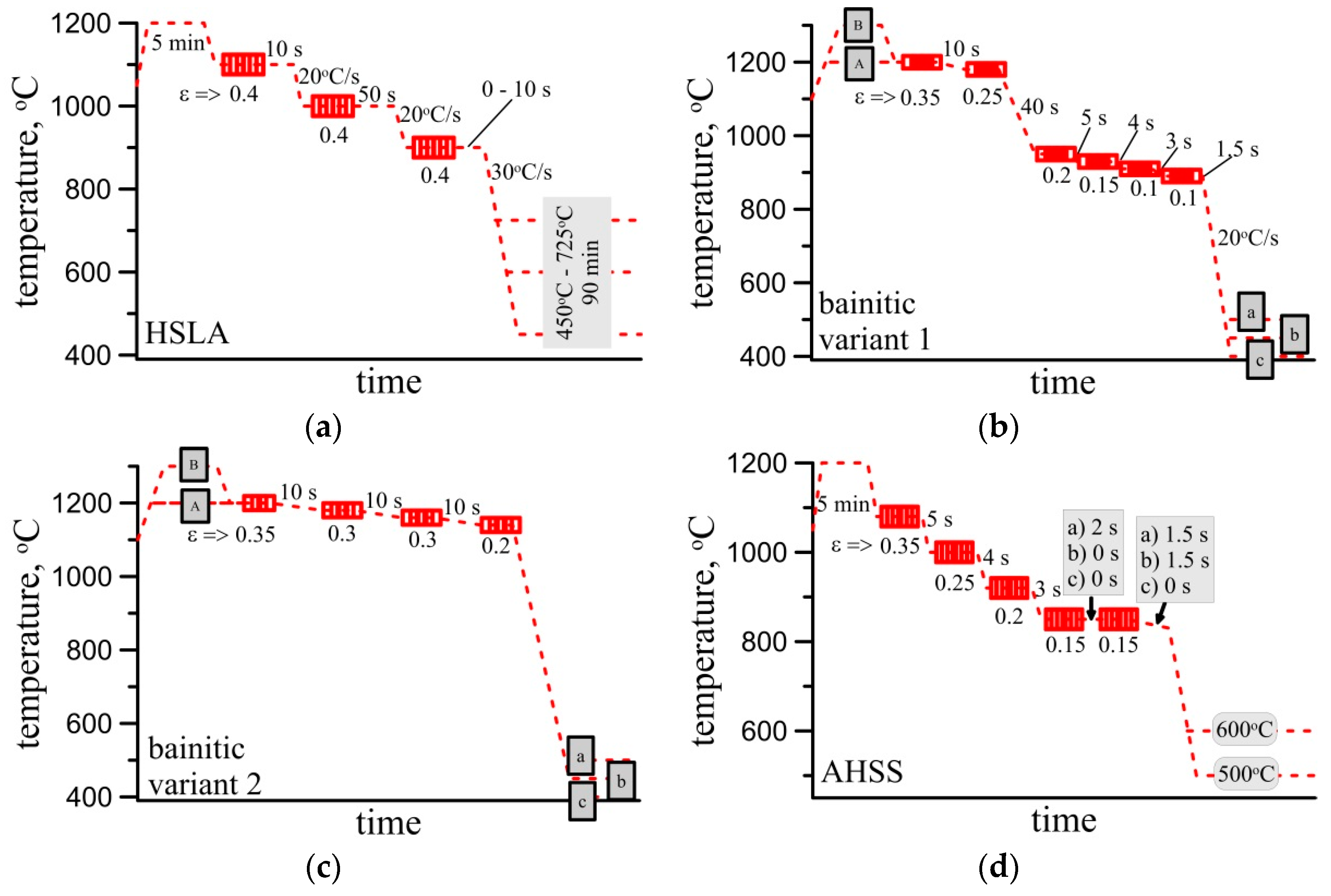
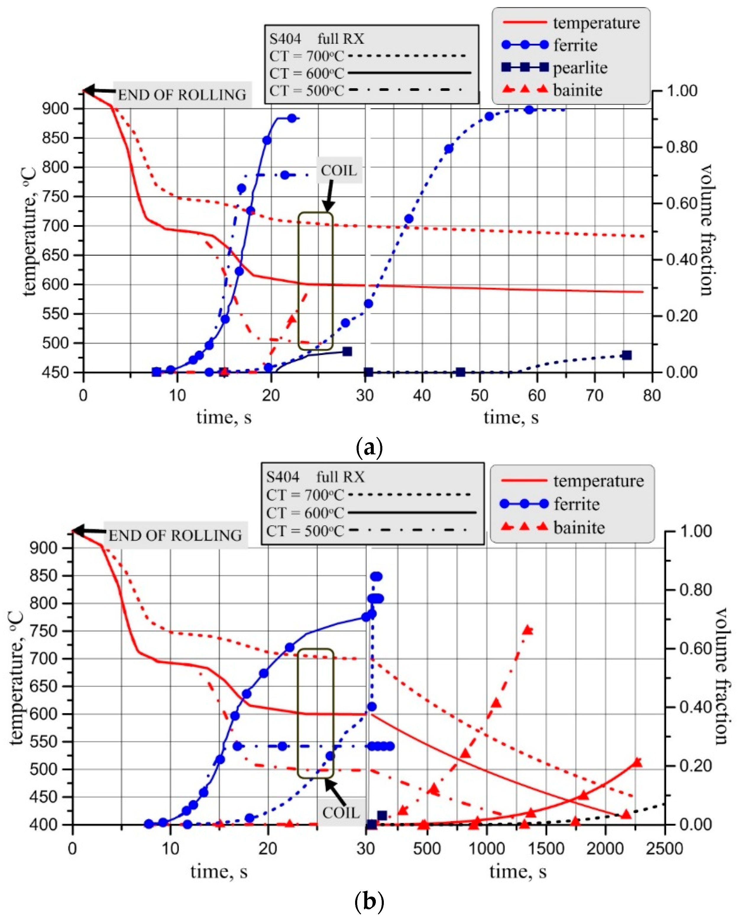
  • HSLA steels: Three passes with the last temperature of 900 °C were considered (Figure 2a). The cooling begun either right after deformation (no recrystallization) or 10 s after deformation (full recrystallization). Cooling from the last deformation temperature to the holding temperature was at the rate of 20 °C/s. Different holding temperatures (400–700 °C) representing cooling in the coil were used for each variant.
  • Bainitic steels: Two variants of physical simulations were considered. In variant 1, presented schematically in Figure 2b, lower temperatures of deformation were applied. Variant 2, presented schematically in Figure 2c, is characterized by higher temperatures of deformation. Two preheating temperatures 1200 and 1300 °C were applied for each schedule, distinguished as A and B variants. Grain size prior to the first deformation (after soaking) was 67 μm for A and 191 μm for B. Cooling from the last deformation temperature to the holding temperature was at the rate of 20 °C/s. Three holding temperatures during cooling, 400, 450, and 500 °C for cooling versions a, b, and c, respectively, were used for each variant.
  • AHSS: Three schedules described in [1] were considered (Figure 2d): The reference schedule (a), the shortest interpass time between the two last deformations (b), and the shortest time between the last deformation and accelerated cooling (c). It allowed to distinguish the austenite microstructure and deformation at the beginning of phase transformations. The coiling temperatures (CT) of 500 and 600 °C were simulated for each schedule.
In each schedule, coiling was reproduced by holding the samples for 90 min in constant temperature, followed by slow cooling in the furnace at 1 °C/s to the room temperature. After performing the tests, the samples were cut for the microstructure characterization (Section 3.2) and mechanical properties measurement (Section 3.3).

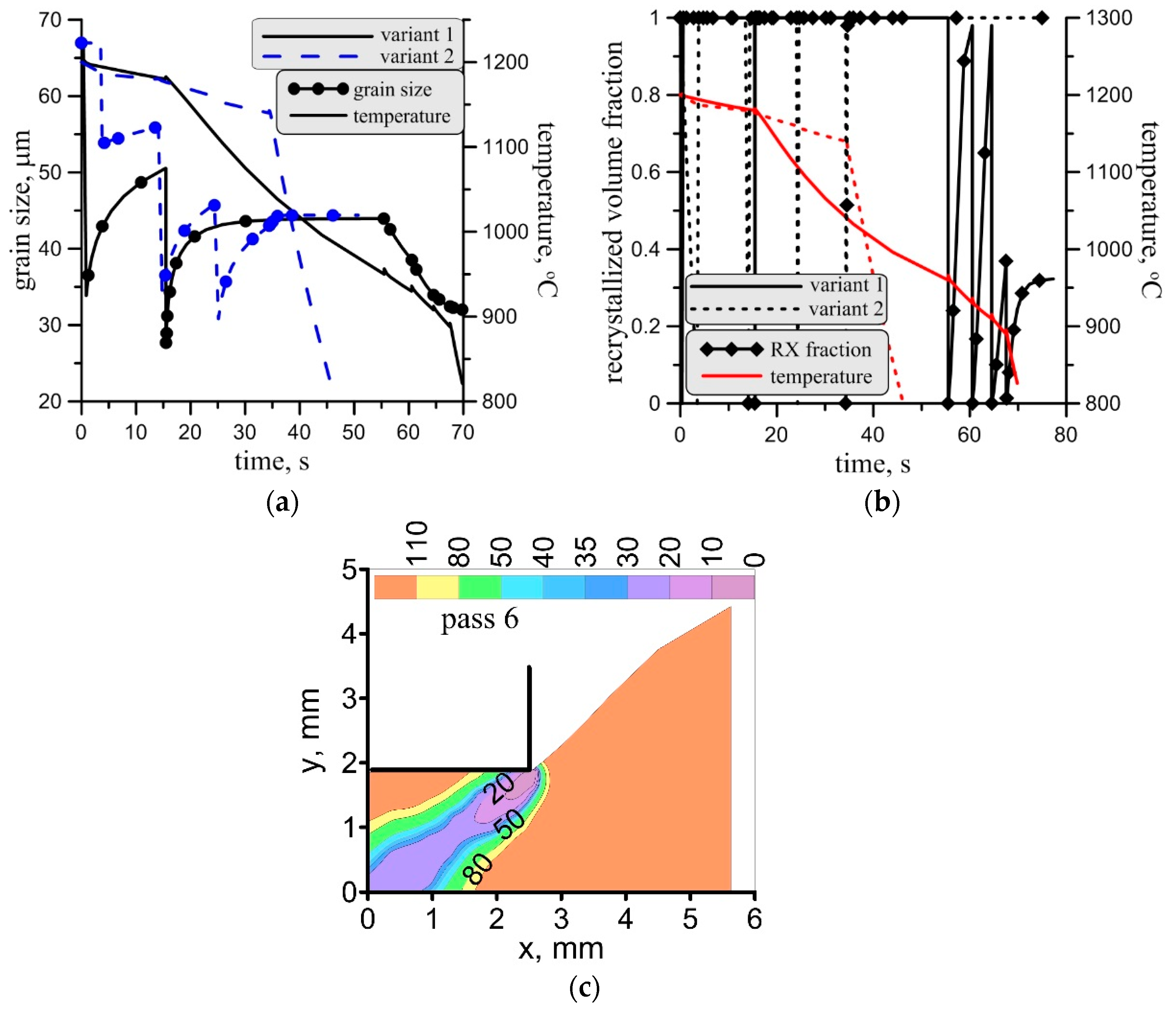
3.2. Microstructures

Samples were quenched at various stages of the process and microstructure was analyzed. Full set of micrographs is presented in [18] and the most important results and conclusions are discussed below.
HSLA steels. All micrographs are presented in the report [18]. Typical FEG-SEM (Field Emission Gun Scanning Electron Microscope) micrographs corresponding to S401 (Nb) and S404 (Nb–Mo) steels, obtained for different coiling temperatures, are shown in Figure 3. In Nb steel, when a high CT is applied, the microstructure is composed by polygonal ferrite (PF) and pearlite (Figure 3a). A combination between quasipolygonal ferrite (QF) and granular ferrite (GF) is formed when coiling temperature decreases (see Figure 3c,e). Different microstructures were observed for S404 (Nb–Mo) steel. For the highest CT, Figure 3b shows that apart from PF, martensite–austenite (MA) microconstituent is obtained. At the intermediate CT of 600 °C, the microstructure is mainly formed by a mixture of QF and GF, even if MA islands are also observed in Figure 3d. Conversely, at the lowest CT of 500 °C (Figure 3f), a fine microstructure of QF and GF units is formed, and no presence of MA regions retained between the transformed phases was detected. It is evident that the presence of non-polygonal transformation products is higher when Mo is added, causing an additional grain refinement.
Optical micrographs corresponding to S404 (Nb-Mo) steel and coiling temperatures of 700 and 600 °C are shown in Figure 3b,d,f. Ferritic matrix is revealed with dark color, while MA islands appear as light color. The morphology and size of the islands differs considerably depending on the coiling temperature. The reduction of coiling temperature results in the formation of finer MA regions (see Figure 3). The microstructural characterization has been extended to S403 (Ti–Mo) steel [18]. As in S404 (Nb–Mo) steel, in S403 the presence of Mo promotes the formation of MA islands at high (700 °C) and intermediate (600 °C) coiling temperatures. However, at a lower coiling temperature of 500 °C, the size of the mentioned MA island is significantly lower.
Bainitic steels. Typical microstructures of the samples subjected to the physical simulation of the rolling process are shown in Figure 4 for variant 1 and in Figure 5 for variant 2. The prior austenite grain size following the last deformation (sample quenched with water) was around 34 μm for steel S405, 30 μm for steel S406, and 48 μm for steel S407. Generally, the microstructure of the steel S406 samples contains allotrimorphic ferrite (<10%), degenerated upper and lower bainite, and blocky martensite. The highest amount of blocky martensite was observed in the S407 steel containing niobium. Microstructures of the samples from steel S405 show that, generally, holding at the highest temperature of 500 °C results in a coarser microstructure and higher blocky martensite fraction compared to holding at 450 and 400 °C. Variant 2 is characterized by the highest last deformation temperature of 1140 °C and the microstructures of the samples subject to all cooling schedules are characterized by smaller size of both, bainitic ferrite and hard martensite particles. Moreover, the distribution of structure constituents is more homogeneous in this case.
AHSS. Based on the different simulated schedules (Figure 2d), microstructures and mechanical properties characterization were performed. Detailed results can be found in [1,18]. Briefly, for the whole samples, ferrite is the main constituent of the microstructure (from 60% to 90% depending on the microalloying and tests conditions). Pearlite and/or martensite are the remaining components of the microstructure. No significant effect of the schedule (a, b, or c) has been observed mainly due the fact that austenite is already highly non-recrystallized for the reference rolling schedule and that the rate of cooling was probably too low (50 °C/s). Interrupted trials, which were performed to observe the austenite microstructure before the two last deformations, revealed recrystallization of the austenite and the average grain size was around 70 µm (Figure 6). In every case, austenite was highly deformed with a quite important grain size leading to similar final microstructures (fine but quite heterogeneous microstructures), see Figure 7.
Analysis of the microstructures for all samples [18] allowed the following conclusions. For Nb steel, volume fraction of ferrite varies from 75% for CT of 500 °C to 85–90% for CT of 600 °C. The addition of Mo (NbMo steel) leads to a lower ferrite volume fraction at the level of 60% for a CT of 500 °C and 70% for CT of 600 °C. Similar observations regarding the effect of molybdenum were made by comparison of the Ti steel and the TiMo steel. The relative fine ferrite microstructure with the grain size at the level of 1–3 μm was obtained for all steels and coiling temperatures.

3.3. Mechanical Properties

PSC samples were large enough to be cut into small samples for tensile tests and hardness measurements. Discussion of results is summarized below.

3.3.1. HSLA

Tensile tests data for all samples were used to determine the effect of the coiling temperature on the mechanical properties, see Section 3.1. Measured yield strength and elongation for various CT are shown in Figure 8. Different strength levels are clearly distinguished depending on the microalloying elements. The highest tensile properties were achieved for S403 steel (Ti–Mo), followed by S404 (Nb–Mo), and S401 (Nb). Looking at the evolution of yield strength, in the steel containing only Nb, it remains approximately constant for the entire range of coiling temperatures. Similar behavior is observed for the tensile strength evolution. However, a different trend can be highlighted when Mo is added (S403 and S404). It is observed that the addition of Mo in Nb microalloyed steels results in increased tensile properties (yield strength), what can be observed mainly at intermediate (600 °C) and low coiling temperature (500 °C). Addition of Mo induces the formation of non-polygonal phases. Such modification of microstructure increments strength through a substructure formation, increases the dislocation density and presence of fine precipitates. The highest yield and tensile strength values are reached at the coiling temperature of 600 °C. This trend can be associated with the presence of a higher fraction of fine precipitates at intermediate coiling temperature (600 °C) in both S404 and S403 steels.
Conversely, the influence of chemical composition on the elongation is almost negligible (see Figure 8b). This suggests that the higher tensile properties reached for the S403 (Ti–Mo) steel do not deteriorate elongation.

3.3.2. Bainitic Steels

The effect of low temperature of deformation (variant 1) compared to high temperature of deformation (variant 2) on the properties of experimental steels is shown in Figure 9 for S405 and S406. Some diversification of strength of the samples is observed depending on the holding (coiling) temperature, such as decreasing the holding temperature results in yield strength decrease and elongation increase, but the lowest strength was obtained for the holding temperature of 450 °C (variants b). Steel S406 (0.18Ti) performs better in terms of strength versus ductility relation. Similar results were obtained for S407 (0.03Nb, 0.18Ti) with slightly lower elongation, which was due to the higher amount of blocky martensite in this steel. The most plausible explanation of all the observation may be connected to the fact that longer time of thermo-mechanical processing results in more intense precipitation of TiC in the austenite. This, however, lowers the precipitation strengthening effect of TiC in bainitic ferrite, see [18] for details.

3.3.3. AHSS

Results of the yield strength measurements are shown in Figure 10. Globally, higher mechanical properties were obtained for a CT of 600 °C. The highest level of these properties was obtained for the TiMo grade and at a CT of 600 °C. The difference of mechanical properties between no-Mo and Mo grades is dedicated to higher fractions of hard phases in the former. In some cases, important gap between mechanical properties was observed without significant variations in the microstructure suggesting an important effect of precipitation strengthening, which seems more pronounced for Ti grades.

4. Models

Multiphysics and multiscale approach was used in the VirtRoll system. Thermal-mechanical coupling was applied in the macro scale. The metallurgical models are responsible for microstructure evolution and phase transformations. These models were solved in the micro scale and full coupling with the macro scale was applied, see Figure 11. Metallurgical models receive information about current local strains, stresses, and temperatures and return transformed volume fraction (X) to the mechanical model and heat due to recalescence (Qrec) to the thermal model.

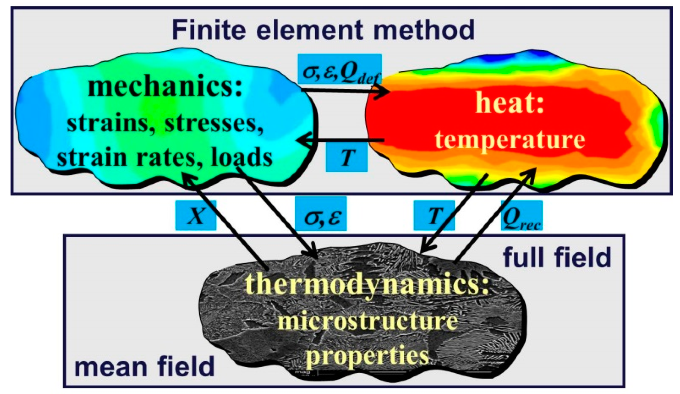
4.1. Mechanical and Thermal Models

Originally, the finite element (FE) model described in [7] was used to calculate mechanical and thermal parameters. Even if a simple stationary FE model with a coarse mesh is used, the computing time for simulation of a single pass is about 2–3 min. Since in the optimization task several passes have to be simulated to calculate one value of the goal function, the search was made for alternative models that can accelerate calculations. The metamodel, which allows for significant decrease in the computing time, is such an alternative. The surface response method was used in the present work to calculate mechanical parameters of the rolling process. Due to the fact that the material flow stress is the main factor, which decides about the accuracy of calculation of forces and torques, the emphasis was put on the accurate identification of the flow stress model. Inverse analysis for the results of the compression tests was performed for each material in the database (Section 3.1 and [18]) and the coefficients in flow stress models were identified. The inverse algorithm described in [21] was applied. Relation between the flow stress (σp) and the average pressure (pav) in rolling has to account for the so called “friction hill” and this relation was described by the metamodel, which follows the concept of Sims [22], who introduced parameter Q representing average pressure-to-flow stress ratio (Q = pav/(p), where a = 2/ 3 ). The data generated by numerous FE calculations for different reductions (r = (h1h2)/h1), roll radii (R) and friction coefficients (μ), were used to find the coefficients in the polynomial function Q = f(r,R,μ). Sensitivity analysis showed that by combining together the effect of geometrical variables in one variable Δ, which is the shape factor of the roll gap (Δ = hav/ld, where hav = (h1 + h2)/2—the average thickness, ld = R h 1 r —the length of the arc of contact, h1 and h2—the entry and the exit thicknesses, respectively), the number of the independent variables can be decreased. Analysis of the results of the FE simulations showed that for a wide range of roll gap parameters the relationship between Q and Δ is linear. Similar approach was used to calculate strain distribution along the thickness of the strip. Approximation of the results of the FE simulations yielded the following equations:
F = σ p l d w ( 1 + 0.572 μ Δ )
ε ( y ) = 2 3 ln ( h h 1 ) [ 1 + 3 ( 0387 y Δ y max ) 2 ]
where, F—rolling force, w—width of the strip, h—strip thickness in the current location, y—coordinate through the thickness with the origin in the strip center, ymax—half of the thickness in the current location.
Remaining rolling parameters, including roll torque, power, and current of the motor are calculated on the basis of the rolling force using conventional equations [17]. Mechanical model is coupled with the thermal model, which is FE non-stationary solution of the heat transfer equation in the plane perpendicular to the rolling direction. The solution domain is moving with the actual strip velocity. The boundary conditions are applied according to the actual cross-section location.

4.2. Material Models

Flow stress, microstructure evolution, and phase transformation models are described in [1] and are not repeated here. As it is seen in Figure 11, metallurgical models of various complexity can be used in the micro scale (either mean field or full field models). Since short computing times are crucial for the design of such processes, only mean field models were used in VirtRoll [1]. Values of coefficients in all the material models for all the investigated steels, which were determined using inverse analysis of plastometric, 2-step compression and dilatometric tests, are given in [1], as well.
Various models describing mechanical properties, including conventional models developed in the second half of the 20th century, e.g., [5], and new models accounting for the effect of precipitation and dedicated to HSLA and AHSS grades, were investigated in this project. The following relation between mechanical properties and the coiling temperature in °C for the HSLA steels was proposed on the basis of approximation of the results of physical simulations described in Section 2:
Re = a 0 + a 1 T c + a 2 T c 2
Rm = b 0 + b 1 T c + b 2 T c 2
where: Re—yield stress, Rm—ultimate tensile strength, both in MPa.
The coefficients in Equations (3) and (4) for the HSLA steels are given in Table 1.
The next model was developed to account for the effect of precipitates in the AHSSs. Assuming summation of various contributions, the yield stress is calculated as:
Re = σ s s + σ g s + σ ρ + σ M A + Δ σ p r e c
where, σss, σgs, σρ, σMA, σprec—contributions of the solid solution, grain size, dislocations, presence of secondary phases, and fine precipitations, respectively.
Contribution of the solid solution depends on the steel chemical composition:
σ s s = σ 0 + 32.3 [ Mn ] + 83.2 [ Si ] + 11 [ Mo ] + 354 [ N f r e e ] 0.5
where, σ0—stress due to lattice resistance or solution hardening or some grain size effects.
Remaining contributions (σgs, σρ, and σMA) are calculated from the equations described widely in the literature and reported also in [1]. The approach reported in [23] was used to calculate the contribution of the grain size. In the proposed model, the precipitation hardening effect does not require information on precipitates size or density. In this model the contribution of precipitation on the total stress depends on the Ti and Nb content and is calculated from the following integral equation:
Δ σ p r e c = K 1 exp [ 1 K 2 lg ( 0 T d T K 4 ) ] K 3
where, M—Taylor factor, b—length of the Burgers vector, G—shear modulus, ρ—dislocation density, fi—low (2° < θi < 15°) and high (θi > 15°) angle boundary fractions, θi— misorientation angle, d 2 o —unit size considering the low angle misorientation criterion, fMAMA volume fraction.
The effect of the thermal path in Equation (7) is accounted for by integration with respect to time. Start temperature for precipitation is calculated from the phase transformation model. Coefficient K1 in Equation (7) is 129.5 and 286 for 0.035% Nb steel and 0.13% Ti steels, respectively. Coefficients K2 = K3 = 2 for both steels. Coefficient K4 is defined as:
K 4 = 10 16 T exp ( 28000 R T )
All the material models mentioned in this Section were implemented into the VirtRoll system data base and simulations of the selected hot strip rolling processes for the investigated steels were performed.

5. Results

5.1. Verification and Validation of the Models

The validation of the roll force and rolling torque models is presented in [18], where good agreement between the measured and calculated parameters was obtained. In the present paper, particular emphasis was put on adjusting the models to be capable to simulate advanced hot rolling routes proposed in the project. The following aspects were of particular importance:
  • Capability to predict material behavior and product properties accounting for different finish rolling temperatures.
  • Decrease of the manufacturing costs by lower alloying elements and improvement of properties using increased cooling capacity—ultra fast cooling (UFC) systems.
  • Capability to predict product properties for multi-phase microstructure, accounting for the properties and morphology of the component phases.
To reach these goals, two sets of simulations were performed. In the first set, PSC tests described in Section 3 were simulated and the results were used for verification and validation of the models. In the second set, physical PSC simulations were reproduced in the VirtRoll system. However, in the deformation the same roll pass schedule was used for all steels. The slab thickness was 40 mm and the following reductions were applied in the subsequent passes: 0.43, 0.4, 0.31, 0.29, 0.25, and 0.18. It gave final thickness of the strip equal to 4mm. The difference between various schedules was in the applied cooling systems.
Numerical simulations of all physical tests in Section 3 were performed using FE model. Authors’ FE code described in [24] was applied. PSC test is characterized by strong inhomogeneity of strains and temperatures, therefore, problems with the interpretation of results of the tests had to be solved. The shape coefficient Δ = h/w (sample thickness-to-die with ratio) changes during the test, which involves changes in the inhomogeneity of deformation. Thus, investigation of the material in the center of the sample, assuming that strains and temperatures at that location are close to the nominal ones, was the commonly used approach. FE simulation of the tests accounted for the heterogeneous character of the deformation and helped in interpretation of the results. All variants of the multi-stage tests in Figure 2 were simulated, and selected results for bainitic steel S405 are presented. Analysis of the strains was performed first, see Figure 12, in which homogeneous strains (εh = 2/ 3 ln(hi/hi+1, where, hi, hi+1—sample height before and after pass i) were compared with strains calculated by the FE code in the center of the sample. It is seen that the latter are higher. The retained strains, which remained due to not complete recrystallization between the passes, are shown in this figure as well. The effect of retained strain is large for variant 1, while it is not observed in variant 2.
Prediction of the microstructure evolution was the next objective. Results of simulations of grain size evolution during the tests in the center of the sample are shown in Figure 13a. Variant 1 leads to much finer grains at the beginning of phase transformations (after the last deformation). Changes of the recrystallized volume fraction are shown in Figure 13b. Full recrystallization was predicted at all stages of the variant 2. On the contrary, partial recrystallization was predicted at the two final stages of the variant 1. In consequence, phase transformations in this variant occur in the non-recrystallized austenite. Distribution of the grain size after last pass of the variant 1 is shown in Figure 13c. This figure confirms strong inhomogeneity of the test.
Predictions of the grain size were compared with the measurements. The grain size was measured in the area 2 mm up from the horizontal axis of symmetry, where the strains are close to the nominal strains in the test. In the case of the bainitic steel S405 comparison of measurements and calculations yielded 35 and 33 μm for the variant 1 and 56 and 63 μm for the variant 2, for calculations and measurements, respectively. Verification of the grain size predictions was performed for all steels and all tests in the project and good accuracy of material models was confirmed.
Simulations of the PSC tests confirmed good predictive capabilities of the material models in the VirtRoll system. In further simulations this system was applied to a conventional hot strip mill with six stands in the finishing train.

5.2. Various Finishing Rolling Temperatures

Typical hot strip rolling mill composed of the furnace, reverse rouging stand, six stand continuous finishing train, laminar cooling and coiler was considered. The laminar flow cooling system is composed of two sections with 40 boxes in each section, see [25] for details. The length of each box is 1 m. The sections are divided into eight zones of three types: intensive, normal, and trimming zone. Distance between the sections is d = 20 m. Schematic illustration of this laminar cooling system is shown in Figure 14. Maximum heat transfer coefficient for each zone of the laminar water cooling was calculated on the basis of equation proposed in [8]. This heat transfer coefficient decreased proportionally with the water flux decrease.
The simulations were performed for all investigated steels, but the results for the bainitic steel S406 only are presented. The strip thickness after the last stand was h6 = 4 mm, strip width was w = 2000 mm, and the velocity in the last stand was v6 = 7 m/s. Two cases were considered, conventional with the finish rolling temperature of 950 °C (case 1) and a new route assuming additional fast cooling devices before stands 5 and 6 (case 2). Calculated time–temperature profiles for both variants are shown in Figure 15a and changes of the austenite grain size are shown in Figure 15b. These data were used as the starting point for simulations of two laminar cooling strategies with coiling temperature 500 and 600 °C. The former is presented in Figure 15a. A typical laminar flow cooling (LFC) system was applied. It was satisfactory to obtain assumed CT of 500 and 600 °C for the considered thickness and velocity of the strip.

5.3. Various Coiling Temperatures

The objective of this set of simulations was to investigate the effect of the coiling temperature in a wide range. The simulations were performed for all steels in the project. Additionally, simulation for the bainitic and HSLA steels was performed for recrystallized (case 1) and not recrystallized (case 2) austenite after rolling. All results for the HSLA NbTiMo steel S404 are shown in Figure 16a. Ferritic-pearlitic microstructure was obtained for the CT 700, 650, and 600 °C. Further decrease of the coiling temperature leads to an increase of the bainite volume fraction in the microstructure [26]. Ferrite transformation is faster but the volume fraction of the ferrite is smaller for the not-recrystallized austenite. Selected example of calculated kinetics of transformation is shown in Figure 17a. Similar results for the bainitic 0.18%Ti–0.2%Mo steel S406 are shown in Figure 16b and Figure 17b. Ferritic–pearlitic microstructure was obtained for the CT = 700 °C and not-recrystallized austenite. Decrease of the coiling temperature leads to an increase of the bainite volume fraction in the microstructure. Similarly to S404, the ferrite transformation is faster but the volume fraction of the ferrite is smaller for the not-recrystallized austenite. Some martensite occurs for the recrystallized austenite and CT = 700 °C. Selected example of calculated kinetics of transformation is shown in Figure 17. Influence of the coiling temperature on the kinetics of transformation is clearly seen in Figure 17a,b.
Following this, selected results for coiling temperature 650 and 550 °C for all steel grades in the project are presented in Figure 18. Ferritic–pearlitic microstructure was obtained for HSLA and AHSS grades and CT = 650 °C while ferrite and bainite was obtained at this coiling temperature for the bainitic steels. Ferritic–bainitic microstructure was obtained for all grades and CT = 550 °C. The strongest effect of microalloying elements was observed for the bainitic steels. In the HSLA grades, addition of Mo caused only slight increase in the pearlite (for CT = 650 °C) or bainite (for CT = 550 °C) volume fraction. In the bainitic steels an addition of Nb + Ti + Mo gave the lowest content of the bainite. In the AHSS grades and CT = 550 °C addition of Ti gives lower volume fraction of the bainite than addition of Nb.
For higher coiling temperature ferritic pearlitic microstructure was obtained for all AHSS and HSLA grades. Some bainite was predicted for bainitic steels. The effect of the microalloying on the phase composition was small for all grades. For lower coiling temperature ferrite with some bainite was obtained for the HSLA grades. Addition of molybdenum or titanium caused an increase in the bainite volume fraction. Ferrite with 35–45% of bainite was obtained for the AHSS grades. The largest bainite volume fraction was obtained for the Nb steel only. Ferrite bainite and martensite was obtained for the bainitic steels. Decrease in the titanium content caused an increase in bainite and martensite in the microstructure.

5.4. Optimization of the Laminar Flow Cooling (LFC) System

Three optimization tasks were implemented into the VirtRoll system, with the following objectives: (i) Uniform distribution of temperature along the strip after rolling, (ii) specific phase fractions after cooling in a coil, and (iii) specific distribution of temperature along the strip before coiling, which allows to minimize microstructure heterogeneity. Only the second task is presented below. The optimization variables are water fluxes on cooling boxes in laminar cooling and rolling schedule in finishing mill, which influences austenite grain size before cooling. The problem is multidimensional and requires the nature-inspired optimization method.
The particular objective of the optimization was to design the cooling technology, which gives the required volume fractions of phases. An example of the optimization for the AHSS11 steel is presented below. The objective was to obtain 30% of hard constituents (martensite and bainite) and minimum of the bainite in steel. Coiling temperature above 400 °C was the constraint. The following objective function was defined:
Φ = w B M ( F B + F M 0.3 ) 2 + w B F B 2
where, wBM, wB—weights, FB, FM—volume fractions of the bainite and martensite, respectively.
In Equation (9) the weights wBM = 0.7 and wB = 0.3 were used. Three cases are presented: case A with v6 = 7 m/s and h6 = 4 mm, case B with v6 = 7 m/s and h6 = 3 mm, and case C with v6 = 5 m/s and h6 = 4 mm. Full recrystallization of the austenite before laminar cooling was assumed. Optimal water flux in all zones for the three cooling cycles is given in Table 2. The final values of the objective function (11) are given in the last column of this table. Since current cooling system does not allow to avoid any bainite in the microstructure in the case C, the final value of the objective was larger for that case. Figure 19 shows temperature changes and kinetics of transformations calculated for the three cases.

5.5. Effect of Precipitation on Mechanical Properties

The model that predicts mechanical properties of strips was tested. Contribution of precipitates to the increase of the yield stress of the AHSS grades was calculated using Equation (7) for cooling schedules characteristic for the hot strip mill. The result is presented in Figure 20. It is seen that contribution of precipitates is larger for the steels containing titanium. These simulations show capabilities of the VirtRoll system to predict properties of strips after rolling and coiling.

6. Conclusions

VirtRoll capabilities can be summarized as follows. It enables optimization of semi product and product properties in metal forming, which due to the application of innovative materials in connection with advanced production technologies, is highly sophisticated nowadays. Prediction of material properties after rolling and cooling usually requires expensive, long-lasting experimental trials, which do not guarantee identifying the optimal technological parameters. The VirtRoll model-based computer system joins functionality of numerical simulations, material modelling, multi-scale modelling, inverse analysis and optimization to minimize costs of design of manufacturing technologies, and maximize semi and final product properties. The system is equipped with advanced numerical models for new generation steels (AHSS, modern bainitic steels, HSLA). The models were identified on the basis of experiments described in Section 3. VirtRoll combines the developed models with database, knowledge base, and inverse solution coupled with optimization techniques in one hybrid computer system. The main advantages and unique functionalities of the system can be summarized as follows:
  • The user friendly interface (GUI), which is usable for engineers who are not IT experts.
  • Advanced physical and numerical models to predict behavior of advanced steels.
  • Guidelines for unconventional production methods.
  • A graphical drag and drop editor that supports flexible design of rolling mill.
  • Database and knowledge base, which essentially support the design of rolling technology.
  • Sensitivity and inverse analyses to support flexible design of strip rolling technology.
  • Combining developed models, database, knowledge base, and inverse into one hybrid computer system.
The case studies presented in the paper confirmed VirtRoll accuracy and reliability, as well as its capability to predict phase composition after various manufacturing routes.

Author Contributions

Conceptualization: all authors; experiments: R.K., P.U., N.I., I.G., R.J.; software: K.B., Ł.R., J.K.; identification: M.P.; validation: K.B., Ł.R., M.P.; simulations: K.B., Ł.R., M.P.; discussion of results: all authors; writing—original draft preparation: M.P.; writing—review and editing: all authors; supervision: Ł.R.; project administration: J.K.

Funding

This research was funded by European Commission, Research Fund for Coal and Steel (RFCS), grant number RFSR-CT-2013-00007.

Conflicts of Interest

The authors declare no conflict of interest.

References

  1. Bzowski, K.; Kitowski, J.; Kuziak, R.; Uranga, P.; Gutierrez, I.; Jacolot, R.; Rauch, L.; Pietrzyk, M. Development of the material database for the VirtRoll computer system dedicated to design of an optimal hot strip rolling technology. Comput. Methods Mater. Sci. 2017, 17, 225–246. [Google Scholar]
  2. Novillo, E.; Cotrina, E.; Iza-Mendia, A.; Lopez, B.; Gutierrez, I. Factors limiting the achievable ferrite grain refinement in hot worked microalloyed steels. Mater. Sci. Forum 2005, 500, 355–362. [Google Scholar] [CrossRef]
  3. Nanba, S.; Kitamura, M.; Shimada, M.; Katsumata, M.; Inoue, T.; Imamura, H.; Maeda, Y.; Hattori, S. Prediction of microstructure distribution in the through-thickness direction during and after hot rolling in carbon steels. ISIJ Int. 1992, 32, 377–386. [Google Scholar] [CrossRef]
  4. Beynon, J.H.; Sellars, C.M. Modelling microstructure and its effects during multipass hot rolling. ISIJ Int. 1992, 32, 359–367. [Google Scholar] [CrossRef]
  5. Hodgson, P.D.; Gibbs, R.K. A mathematical model to predict the mechanical properties of hot rolled C-Mn and microalloyed steels. ISIJ Int. 1992, 32, 1329–1338. [Google Scholar] [CrossRef]
  6. Pietrzyk, M. Finite element based model of structure development in the hot rolling process. Steel Res. 1990, 61, 603–607. [Google Scholar] [CrossRef]
  7. Pietrzyk, M. Through-process modelling of microstructure evolution in hot forming of steels. J. Mater. Process. Technol. 2002, 125, 53–62. [Google Scholar] [CrossRef]
  8. Uranga, P.; Fernandez, A.I.; López, B.; Rodriguez-Ibabe, J.M. Modeling of austenite grain size distribution in Nb microalloyed steels processed by thin slab casting and direct rolling (TSDR) route. ISIJ Int. 2004, 44, 1416–1425. [Google Scholar] [CrossRef]
  9. Matlock, D.K.; Krauss, G.; Speer, J.G. New microalloyed steel applications for the automotive sector. Mater. Sci. Forum 2005, 500, 87–96. [Google Scholar] [CrossRef]
  10. Lotter, U.; Schmitz, H.-P.; Zhang, L. Structure of the metallurgically oriented modelling system TK-StripCam for simulation of hot strip manufacture and application in research and production practice. J. Phys. IV France 2004, 120, 801–808. [Google Scholar]
  11. Andorfer, J.; Auzinger, D.; Hirsch, M.; Hubmer, G.; Pichler, R. VAI-Q strip-an online system for controlling the mechanical properties of hot rolled strip. In Proceedings of the IFAC Workshop on Automation in Mining, Mineral and Metal Processing, Cologne, Germany, 1–3 September 1998; pp. 325–330. [Google Scholar]
  12. Trowsdale, A.J.; Randerson, K.; Morris, P.F.; Husain, Z.; Crowther, D.N. MetModel: Microstructural evolution model for hot rolling and prediction of final product properties. Ironmak. Steelmak. 2001, 28, 170–174. [Google Scholar] [CrossRef]
  13. Loffler, H.; Doll, R.; Poppe, T.; Sorgel, G.; Holtheuer, U.; Zouhar, G. Control of mechanical properties by monitoring microstructure. AISE Steel Technol. 2001, 1, 44–47. [Google Scholar]
  14. Ibrahim, M.; Shulkosky, R. Simulation and development of Advanced High Strength Steels on a hot strip mill using a microstructure evolution model. HSMM Appl. AHSS 2007, 1, 1–12. [Google Scholar]
  15. Donnay, B.; Herman, J.C.; Leroy, V.; Lotter, U.; Grossterlinden, R.; Pircher, H. Microstructure evolution of C-Mn steels in the hot deformation process: The STRIPCAM model. In Proceedings of the Modelling of Metal Rolling Processes, London, UK, 9–11 December 1996; Beynon, J.H., Ingham, P., Teichert, H., Waterson, K., Eds.; Institute of Metals: London, UK; pp. 23–35. [Google Scholar]
  16. Kuziak, R.; Pietrzyk, M. Physical and numerical simulation of the manufacturing chain for the DP steel strips. In Proceedings of the Steel Research International Special Edition Conference, ICTP, Aachen, Germany, 25–30 September 2011; pp. 756–761. [Google Scholar]
  17. Rauch, L.; Bzowski, K.; Kuziak, R.; Kitowski, J.; Pietrzyk, M. The off-line computer system for design of the hot rolling and laminar cooling technology for steel strips. J. Mach. Eng. 2016, 16, 27–43. [Google Scholar]
  18. Pietrzyk, M.; Larzabal, G.; Uranga, P.; Isasti, N.; Jacolot, R.; Rauch, L.; Kuziak, R.; Diegelmann, V.; Kitowski, J.; Gutierrez, I.; et al. Virtual Strip Rolling Mill VirtRoll; European Commission Research Programme of the Research Fund for Coal and Steel, Technical Group TGS 4, Final Report from the Project RFSR-CT-2013-00007; European Commission: Luxembourg, 2017.
  19. Krol, D.; Wrzeszcz, M.; Kryza, B.; Dutka, L.; Kitowski, J. Massively scalable platform for data farming supporting heterogeneous infrastructure. In Proceedings of the 4th International Conference on Cloud Computing, GRIDs, and Virtualization, IARIA Cloud Computing, Valencia, Spain, 27 May–1 June 2013; pp. 144–149. [Google Scholar]
  20. Wong, S.F.; Hodgson, P.D.; Thomson, P.F. Comparison of torsion and plane-strain compression for predicting mean yield strength in single-and multiple-pass flat rolling using lead to model hot steel. J. Mater. Process. Technol. 1995, 53, 601–616. [Google Scholar] [CrossRef]
  21. Szeliga, D.; Gawąd, J.; Pietrzyk, M. Inverse analysis for identification of rheological and friction models in metal forming. Comput. Methods Appl. Mech. Eng. 2006, 195, 6778–6798. [Google Scholar] [CrossRef]
  22. Sims, R.B. The calculation of roll force and torque in hot rolling mills. Proc. Inst. Mech. Eng. 1954, 168, 191–200. [Google Scholar] [CrossRef]
  23. Iza-Mendia, A.; Gutierrez, I. Generalization of the existing relations between microstructure and yield stress from ferrite–pearlite to high strength steels. Mater. Sci. Eng. A 2013, 561, 40–51. [Google Scholar] [CrossRef]
  24. Pietrzyk, M. Finite element simulation of large plastic deformation. J. Mater. Process. Technol. 2000, 106, 223–229. [Google Scholar] [CrossRef]
  25. Pietrzyk, M.; Kusiak, J.; Kuziak, R.; Madej, L.; Szeliga, D.; Golab, R. Conventional and multiscale modelling of microstructure evolution during laminar cooling of DP steel strips. Metal. Mater. Trans. B 2014, 46B, 497–506. [Google Scholar]
  26. Jacolot, R.; Huin, D.; Marmulev, A.; Mathey, E. Hot rolled coil property heterogeneities due to coil cooling: Impact and prediction. Key Eng. Mater. 2014, 622–623, 919–928. [Google Scholar] [CrossRef]
Figure 1. An overview of a system-supporting study on the workflow of the hot strip rolling processes.
Metals 09 00737 g001
Figure 2. Simulated rolling schedules for HSLA steels (a), bainitic steels (b,c), and AHSS grades (d).
Metals 09 00737 g002
Figure 3. Typical FEG-SEM micrographs corresponding to S401 (Nb) steel (a,c,e) and S404 (Nb–Mo) steel (b,d,f), coiled at 700 °C (a,b), at 600 °C (c,d), and 500 °C (e,f).
Metals 09 00737 g003
Figure 4. Sample images of the microstructure for heat S405 (a,c,e) and S406 (b,d,f) at plane strain compression (PSC) deformation, variant 1a (a,b), variant 1b (c,d), and variant 1c (e,f).
Metals 09 00737 g004
Figure 5. Sample images of the microstructure for heat S405 (a,c,e) and S406 (b,d,f) at PSC deformation, variant 2a (a,b), variant 2b (c,d) and variant 2c (e,f).
Metals 09 00737 g005
Figure 6. Microstructure before the next to last deformations for the Nb steel (a) and the NbMo steel (b).
Metals 09 00737 g006
Figure 7. Selected microstructures for the Nb steel (a,c) and the TiMo steel (b,d) with a coiling temperature of 500 °C (a,b) and 600 °C (c,d); rolling schedule (a) in Figure 2d.
Metals 09 00737 g007
Figure 8. Yield strength (a) and elongation (b) of HSLA steels after various coiling temperatures.
Metals 09 00737 g008
Figure 9. Yield strength (a) and elongation (b) of bainitic steels after various variants of physical simulation.
Metals 09 00737 g009
Figure 10. Yield strength of AHSS samples for various coiling temperatures and variants a, b, and c in Figure 2d.
Metals 09 00737 g010
Figure 11. The idea of the multiphysics modelling of metal forming, σ—stress, ε—strain, T—temperature, Qdef—heat generated due to plastic work, Qrec—heat generated due to transformations, X—volume fractions of phases.
Metals 09 00737 g011
Figure 12. Homogeneous strains (εh), strains in the center of the sample calculated by the finite element (FE) code and retained strains for bainitic steel variant 1 (a) and variant 2 (b).
Metals 09 00737 g012
Figure 13. Changes in the temperature and the grain size (a) and the recrystallized volume fraction (b) in the center of the sample during both investigated variants for bainitic steel and distribution of the grain size after the last pass of the variant 1 (c).
Metals 09 00737 g013
Figure 14. Schematic illustration of the laminar cooling system for steel strips. Number of boxes in each zone as well as the maximum water flux in various zones are given in the figure.
Metals 09 00737 g014
Figure 15. Time temperature profiles (a) and grain size changes (b) for cases 1 and 2, and kinetics of the transformations for the cooling temperature 500 °C (c) and 600 °C (d).
Metals 09 00737 g015
Figure 16. Effect of the coiling temperature on the volume fractions of phases for the HSLA NbTiMo steel S404 (a) and bainitic TiMo steel S406 (b).
Metals 09 00737 g016
Figure 17. Kinetics of transformation for S404 (a) and S406 (b) grades for various coiling temperatures.
Metals 09 00737 g017
Figure 18. Phase composition of various steel grades after coiling at 650 °C (a) and 550 °C (b).
Metals 09 00737 g018
Figure 19. Temperatures and kinetics of transformations for the three optimal cooling schedules: (a) h6 = 4 mm and v6 = 7 m/s, (b) h6 = 3 mm and v6 = 7 m/s, (c) h6 = 4 mm and v6 = 5 m/s.
Metals 09 00737 g019
Figure 20. Contribution of precipitates to the increase in the yield stress of the AHSS grades calculated using Equation (7) for cooling schedules characteristic for the hot strip mill.
Metals 09 00737 g020
Table 1. The coefficients in equations describing mechanical properties of the HSLA steels.
Steela0a1a2b0b1b2
S401 (Nb)−951.414.7938−0.004−671.314.068−0.0034
S403 (Nb + Mo)−4214.216.442−0.0136−4380.517.247−0.0143
S404 (Ti + Mo)−3197.912.994−0.0111−3184.213.085−0.0111
Table 2. Water flux (m3/h) in each zone of the laminar cooling for the cycles A, B, and C.
Cycle1 I2 I3 N4 N5 I6 I7 N8 TΦ
A156180135001803002400.015
B10512096001262251680.015
C9010569090126216660.04

