Hot Rolling Simulation System for Steel Based on Advanced Meshless Solution


1
Laboratory for Simulation of Materials and Processes, Institute of Metals and Technology, Lepi pot 11, 1000 Ljubljana, Slovenia
2
Laboratory for Fluid Dynamics and Thermodynamics, Faculty of Mechanical Engineering, University of Ljubljana, Aškerčeva 6, 1000 Ljubljana, Slovenia
*
Author to whom correspondence should be addressed.
Metals 2019, 9(7), 788; https://doi.org/10.3390/met9070788
Submission received: 23 May 2019
/
Revised: 8 July 2019
/
Accepted: 14 July 2019
/
Published: 16 July 2019
(This article belongs to the Special Issue Researches and Simulations in Steel Rolling)
Abstract
:In this work, a rolling simulation system for the hot rolling of steel is elaborated. The system is capable of simulating rolling of slabs and blooms, as well as round or square billets, in different symmetric or asymmetric forms in continuous, reversing, or combined rolling. Groove geometries are user-defined and an arbitrary number of rolling stands and distances between them may be used. A slice model assumption is considered, which allows the problem to be efficiently coped with. The related large-deformation thermomechanical problem is solved by the novel meshless Local Radial Basis Function Collocation Method. A compression test is used to compare the simulation results with the Finite Element Method. A user-friendly rolling simulation application has been created for the industrial use based on C# and .NET framework. Results of the simulation, directly taken from the system, are shown for each type of the rolling mill configurations.
Keywords:
rolling; steel; numerical simulation; slice model; grooves; radial basis functions; meshless method1. Introduction
The rolling of steel has always been an important research subject due to a variety of rolled products in use by humankind. It requires an interdisciplinary knowledge of steel metallurgy, deformation theory, and heat transfer. Until the 1970s, understanding of rolling was mainly based on experimental knowledge. As a result, there have been many empirical relations developed [1,2,3], with some still in use for making reasonable predictions of the process [4,5]. Material process modelling and simulation took place right after the development of suitable numerical methods and extensive use of the computers. The first numerical formulation of plasticity was introduced using the Finite Element Method (FEM) in 1962 [6]. Later, the first elastoplastic analysis of plane strain and plane stress problems was done in 1973 [7]. The first rigid-plastic rolling simulation was done in 1982 in Japan [8], and the first multipass rolling simulation was done in 1992 [9]. A detailed history chart of the rolling simulation progress can be found in Reference [10]. Meshless Methods (MM), an alternative to FEM that do not require meshing and do not experience problems with large element distortions, represent one of the most fast-developing fields of computational mechanics. Several strong and weak formulations of MM with different trial and weight functions have been applied to solid mechanics problems, such as element-free Galerkin method [11], finite point method [12], and local Petrov-Galerkin method [13]. A comprehensive description of these methods, together with assessment of their characteristics for solid mechanics, can be found in [14]. MM are found various applications, as well as in the simulation of material forming, starting from the early 1990s. A review of these applications is discussed in [15].
In this paper, recent developments of our comprehensive rolling simulation system, which includes a rolling-specific and user-friendly man-machine interface, MM solution procedure, and a comprehensive set of technologically important graphical outputs for simulating different types of rolling mills, is explained. The system was previously able to simulate schedules with flat, round [16], and non-symmetric grooves [17]. The upgrades of the system, which allow the system to simulate the reversing rolling mill process, are of a particular focus in the present paper. Rolling schedules are distinguished as flat, round, or reversing rolling types. Each type may consist of multiple rolling schedules. Material model, roll gaps, and type of the grooves, as shown in Figure 1, are all user-defined, and this helps the user to make his own sensitivity studies. Another major importance of this paper is to provide the reader with both the details of the physical model, as well as the details of the numerical solution, which are rare to see in recent rolling publications. The reason is that a vast majority of the rolling simulations employ well-known and well-optimized commercial FEM-based codes.
The present rolling simulation system involves coupled thermal and mechanical governing equations, defined on a 2D plane strain deformed physical domain. The calculations are made for one computational slice at a time that follow one after another through the rolling path. The thermomechanical equations are solved in a coupled way using meshless Local Radial Basis Function Collocation Method (LRBFCM). This method uses the unknown fields interpolated by Radial Basis Functions (RBF) through the collocation points, which are smartly distributed over the computational domain and boundary. For each unknown at a collocation point, the interpolation is done by considering only its neighboring points, which form a local influence domain. LRBFCM has been previously shown to be a successful method to solve complex multi-physics problems [18] and thermo-elasticity [19]. A slice model assumption has been used for rolling simulations, since the pioneering application of FEM [20]. LRBFCM was first employed in a rolling simulation using a hypothetic elastic material [21] and later using the von-Mises plastic flow rule [22]. Both material models have been applied to multiple rolling schedules. Recently, simulations with non-symmetric groove types were validated with the industrial results [17]. In the present paper, a reversing rolling mill is simulated using a slice model assumption and a meshless solution procedure. The reverse rolling schedules usually take place before finishing rolling mill. The reverse rolling mill reductions are usually very high, and it is possible for the change in rolling direction to be accompanied with 45 or 90 degrees of rotation between the passes, and the number of the passes could be very high. The main contribution of this work is the demonstration of the simulation of these possibilities. Thus, the present rolling simulation system allows for the most complete rolling mill virtual path design, tuning of rolling parameters, and their optimization.
Later in this paper, the physical model, solution procedure, numerical implementation, compression test comparison of our meshless approach with FEM, and the simulation results for flat, round, and reversing mills are shown.
2. Solution Method
The slice model assumption, governing equations, corresponding initial and boundary conditions, and the numerical solution is explained in this section.
2.1. Slice Model
Rolling of steel is a very complex 3D solid mechanics problem. Therefore, the numerical simulation of rolling requires an extremely high computational power and time, proportional with the desired accuracy. In order to optimize the computational time, allowing the technologist many alternative simulations in a short time, a 2D slice physical model is chosen and schematically depicted in Figure 2. The deformation for any slice toward the rolling direction obeys the homogeneous plane strain assumption [1,9]. This assumption is also known as homogeneous compression, in which the planes remain planes as described by Lenard [15]. The material flow is constant, and the slice model assumption becomes more realistic, as the slices are positioned very close to each other over the contact length. The increased rolling-direction velocity of the deformed slice is proportional to the decrease in the slice area.
2.2. Governing Equations
The coupled thermal and mechanical governing equations that follow are solved in their strong form, consistent with the collocation meshless solution procedure used. The adjacent thermal and mechanical boundary conditions depend on the position in the rolling mill.
2.2.1. The Thermal Model
Heat transfer equation for the slice is defined as
where ρ, cp, T, t, k, stand for density, specific heat, temperature, time, thermal conductivity, and internal heat generation rate due to deformation, defined as
where η is Taylor-Quinney parameter, defining the amount of work turning into heat, is effective stress, and is effective strain. At the boundaries of the computational domain, boundary condition of the third type is applied,
Boundary is divided into contacting and non-contacting parts. At each of these parts, a corresponding heat transfer coefficient h is defined. It takes into account the mechanical contact to the roll in the contacting part. Otherwise, the convection and the radiation to the environment of the rolling mill are taken into account in h. If a part of the boundary coincides with the symmetry axis, then at this boundary, the heat flux is set to 0 W/m2. Accordingly, the reference temperature Tref is also adjusted depending on the contacting and non-contacting status of the boundary part. The solution of Equation (1) also requires knowledge of the initial temperature distribution.
2.2.2. The Mechanical Model
The mechanical equilibrium in steady state is
where L is the 2D derivative operator matrix, is the stress vector, and is the body force vector, neglected in the present rolling context. This equation may also be written in terms of displacement vector u using the stiffness matrix C, consisting of Young’s modulus and Poisson ratio for elastic material or effective stress-effective strain relation for plastic material [23].
Any point at the boundary of a slice can be subject to prescribed displacement or traction
where n is the unit normal vector. The thermal and the mechanical models are coupled through temperature depended material properties which effect the deformation behavior.
2.3. Thermomechanical Solution Procedure
Nowadays, FEM is the most commonly used numerical method for solving engineering solid mechanics problems. This may be due to the existence of many available successful commercial and open-source applications. However, there are many other novel ways of solving partial differential equations numerically, such as Lattice-Boltzmann methods, particle methods, and a huge spectrum of other meshless methods. The MM, employed in the present paper [19], is new compared to FEM. However, it is also capable of successfully solving large deformation problems.
The temperature field in the thermal model and the displacement vector components in the mechanical model are discretized and solved in the following way. The solution is for all rolling type variants is based on the 2D Cartesian coordinate system. Instead of a grid generation over the computational domain such as in FEM, collocation nodes without any special geometrical connectivity are located over the domain and at the boundaries. An unknown scalar or vector component field θ(p) at position p = pxix + pyiy (px, py are Cartesian components and ix, iy are orthonormal Cartesian base vectors) is interpolated with multiquadric RBF Ψ(p) over neighboring (N = 5) nodes in the thermal model, and (N = 7) nodes in the mechanical model, as shown in Figure 3, together with the augmented first order (Np = 3) polynomials ϑ(p)
xmax and ymax are the maximum horizontal and vertical distances between the considered nodes. px0, py0 are the coordinates of the central node inside the influence domain, c is the multiquadric shape parameter, set to 32 in the present simulations. The collocation thus reads
The first partial derivatives are obtained from the interpolation as follows
Similarly, the second partial derivatives can also be obtained. Explicit solution of the governing equation of the thermal model is considered
The temperature field in the thermal model is interpolated in sense of Equation (8)
Depending of the collocation node position, discrete form of boundary or governing equation is written together with the neighboring nodes. This process is repeated for each local influence domain for each time step. The unknown collocation coefficients () are determined through the equation values and the same coefficients are used for the temperature value interpolation inside each local influence domain. More details of this solution are described in [24].
In the mechanical model, collocation is applied to the displacement vector components
The governing equations and the boundary conditions are rewritten in discrete form for each collocation node by considering its neighboring points. In this paper, the 3 × 3 stiffness matrix C introduced in Equation (5), is used as defined in [25]. A system of equations with dimension 2N × 2N and N is the number of the collocation nodes, is assembled to solve the displacement field U from
B is the adjacent vector which contains the boundary values. This equation, however, may not be always trivial to solve due to nonlinear plastic material properties (). The solution matrix A may contain the unknown displacement, which is yet to be solved. In this case an iterative solution is applied. Commercial FEM codes use Newton-Raphson or modified Newton-Raphson method for the convergence of the solution. This requires partial derivatives of the left side of the equilibrium to create an additional Jacobian matrix. The iterative solution chosen here is the direct iteration due to its implementation and solution simplicity. At each iteration step j, the material properties are linearized and updated until converge is achieved in the following form
The scheme of the direct iteration is shown in Figure 4. An effective stress-effective strain relation is required for the iterative solution.
2.4. Collocation Node Distribution
A 2D physical domain is defined as a cross-section of the initial steel strand to be rolled. Collocation nodes are distributed uniformly at the beginning in the case that the initial slice geometry allows this. Otherwise, iterative Elliptic Node Generation (ENG), elaborated in [26], is used.
However, when the diamond-like groove shapes are used in the rolling schedule, the strand is rotated 45 degrees before the passes. If there is also a quarter symmetry, the physical domain becomes a triangle instead of a rectangle. A mapping algorithm based on ENG is used to transform the uniformly distributed nodes on a rectangle to a triangular configuration as demonstrated in Figure 5.
3. Simulation Results
The represented rolling simulation system is written in C# and compiled in Microsoft Visual Studio Express 2015 for Windows desktop and works with Microsoft .NET framework version 4.0 or above. An additional Math.Net version 3.8.0 library is linked in the code for efficient solving of the systems of equations. All simulations in the present paper (including those with FEM for verification) have been run on i7 2.6 GHz processor platform with 16 GB memory, which typically requires 1 h CPU time for a rolling simulation.
A comparison of the present solution procedure with FEM code Deform 2D [27] is made in Section 3.1 in terms of deformation and internal heat generation as an addition to the many test cases run previously. The material properties used in this comparison are given in Appendix A. Afterwards, simulation of 3 different rolling schedules is considered and presented. A flat rolling schedule for slab rolling is given in Section 3.2. Afterwards, in Section 3.3, a schedule consisting of oval and round grooves is tackled to obtain a round billet at the end. The third schedule, given in Section 3.4, represents a reversing rolling mill, where the billet passes through the same rolling stand back and forth and is in-between rotated for 45 or 90 degrees.
In the current version of the simulation system, deformation in each pass is analyzed individually using a single material model. It is not possible to experimentally determine the change in the material properties after each roll pass. However, the reduction rates are quite high, and rolling takes place at very high temperatures. In the present simulations, we assumed that the critical strain to activate dynamic recrystallization is reached at each pass, respectively. The contact time at the first pass is around 0.05 s and decreases after each roll pass. This leads to very high strain rates, which are the main triggers of the dynamic recrystallization together with the high temperatures. Nevertheless, more sophisticated material models that will include also strain hardening can be added in the future.
All necessary data for reconstruction of the rolling process in this paper are given in the description of the examples and in Appendix A.
3.1. Comparison of the LRBFCM Solution with FEM in Terms of Deformation and Internal Heat Generation
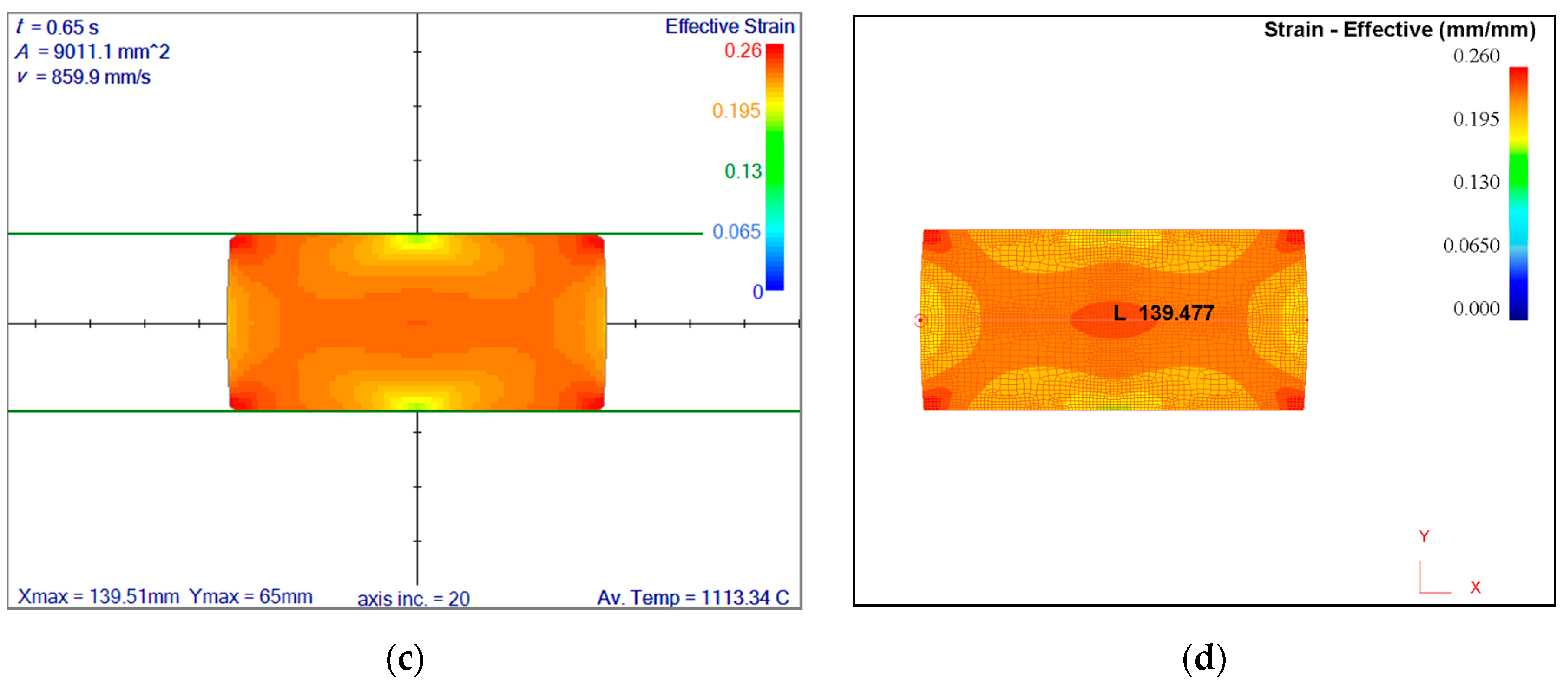
A fair comparison of FEM and LRBFCM is achievable for simple benchmark tests in practice. The LRBFCM algorithms used in this rolling simulation system have been previously compared extensively with the analytical solutions, such as bending of a cantilever beam [16], bending of a beam by uniform load [28], expansion of a cylindrical tube [28], linear compression-tension example [28], and hole in an infinite plate [16]. A systematic assessment of the MM solution procedure was based on a spectrum of relevant comparisons with the well-established FEM: Compression and tension test [16], flat rolling comparison [21], oval rolling comparison [28], width spread comparison [21], and convective cooling example [16]. In this paper are the previous comparisons, complemented in terms of internal heat generation as a consequence of the plastic deformation. A flat rolling situation is chosen to make a comparison between LRBFM and FEM results. Initial cross-section of the steel bloom is 126 × 81 mm and the effective stress-effective strain relation is defined as . The strand is compressed (reduced) from 85 mm to 65 mm height in 0.65 s. A uniform temperate field with 1100 °C is assumed initially. The Coulomb model of friction is applied at the contact surfaces with the coefficient of friction 0.1, based on the experimental results for hot rolling of steel [1]. Thermal insulation is assumed at the boundaries and the only temperature increase is based on the internal heat generation. After the deformation, the size is calculated to be 139.51 × 65 mm by LRBFCM and 139.48 × 65 mm by FEM. Comparisons of deformed shapes and temperature increase are shown in Figure 6. The maximum temperature increase is approximately 15 degrees in both cases. Five-hundred forty-four collocation nodes are used in the present meshless method in Figure 6c, and 950 quadrilateral finite elements are used in Figure 6d. The computational time spent by both numerical methods for solving the above described test is comparable, i.e., 20 CPU seconds.
The stability of meshless method and FEM is very hard to compare directly due to the background optimization process of the commercial FEM code, such as the one employed here for comparison. It has been observed that a FEM based simulation may slightly change the boundary conditions in order to obtain more stable results. It is also possible to encounter instability issues during LRBFCM simulations that are in the present system automatically adjusted. Therefore, it may be necessary to adjust several simulation parameters to increase the stability. These parameters are primarily the density of the vertical and the horizontal node distribution, slice position increments toward the rolling direction, and redistribution of the collocation nodes after a completed roll pass. When the reduction is expected to be high, then it is better to slightly reduce the node density on the reduction axis. If the length of the roll contact will extend from a point to an important part of the boundary, then it is better to set the default incremental slice movement from 5 mm to 1 mm or even less. This action, done automatically, increases the computational time, as well as the numerical stability. Such fine slice movement is typically used when a square to oval or round schedule is simulated, like that shown in Figure 9. When two consecutive rolling stands with the same orientation, such as vertical-vertical or horizontal-horizontal, are used in the schedule, then it is better to redistribute the collocation nodes in between these passes. In both methods, redistribution of the collocation nodes or remeshing is not desired, but it is a necessity in order to continue with the large deformation simulations.
In both simulations, ideal plastic material model with von-Mises flow rule is considered and the same yielding function is used. The nonlinear material model requires iterative solution for each deformation step. FEM code uses Newton-Raphson approach, while the LRBFCM model presented here uses direct iteration due to its simplicity and compatibility with the meshless solution procedure. The discretization of the physical domain is done by quadrilateral elements in FEM and collocation nodes in LRBFCM. It is much easier to distribute the collocation nodes over a domain and slightly move them when necessary as compared to the remeshing procedures employed in FEM. Adding or removing of the computational nodes where it is needed is a quite simple process in the present MM.
3.2. Rolling Simulation Results 8 Flat Rolls
A flat rolling schedule is chosen for demonstration of the simulation system and the results are given in terms of effective strain fields as show in Figure 7. The initial size of the steel slab is 200 × 48 mm, and five of eight rolls are horizontal and flat. Three vertical rolls have specific groove shapes, as seen in figures with groove surface lines. All the contacting groove surface lines, starting from the first contact until the last contact, are drawn. There are 1915 collocation nodes uniformly distributed, and all the rolls have 460 mm diameter. The effect of coefficient of friction on deformation during each roll pass is also studied. The same rolling schedule, as shown in Figure 7, is used, and the results are demonstrated in Figure 8. There is noticeable influence on deformation parameters as the stand number increases. However, during the first a few passes, the effect is low.
3.3. Rolling Simulation with 7 Oval Rolls
The second demonstration of the rolling simulation system is shown for simulating round schedules, which consists of seven passes (oval, oval, round, oval, round, oval, round) with the roll diameter 460 mm. There are 1365 collocation nodes uniformly distributed over the initial slice. The main difference between the flat and the oval/round simulations is the node distribution, which is the case of oval distributions based on ENG. ENG yields very stable results, especially for local interpolation such as the present one, since the orthogonality in-between the neighboring nodes is as high as possible and the nodes are positioned on imaginary lines perpendicular to the boundary surface. If the boundary surface is round or oval, which is the case in round rolling, it is not possible to simulate this type of rolling without redistributing the colocation nodes. Simulation results in terms of displacement field at each pass are shown in Figure 9, where a billet with an initial cross-section 72 × 72 mm is rolled into a circular bar with 40 mm diameter.
3.4. Rolling Simulation of Reversing Rolling Mill with 10 Passes
In the previous two simulations, the slice positions and positions of the rolling stands were known and determined before the simulation starts. However, for reversing rolling mill, the actual travelled distance and time of the slice can only be determined after each deformation step. There are altogether 10 passes and the simulation results are separated into two sections. The first section includes the first five passes and the second section includes the passes from six to 10.
3.4.1. Selection of the Position in the Reversing Rolling
The reversing rolling mill simulation differs much from the finishing rolling mill simulation, especially when the slice model is considered. Changing the rolling direction at each pass creates a difference in slice’s position and time relation. A user-defined option with three choices is considered in the simulation system, as demonstrated in Table 1.
3.4.2. Reversing Rolling Mill Simulation–First Section
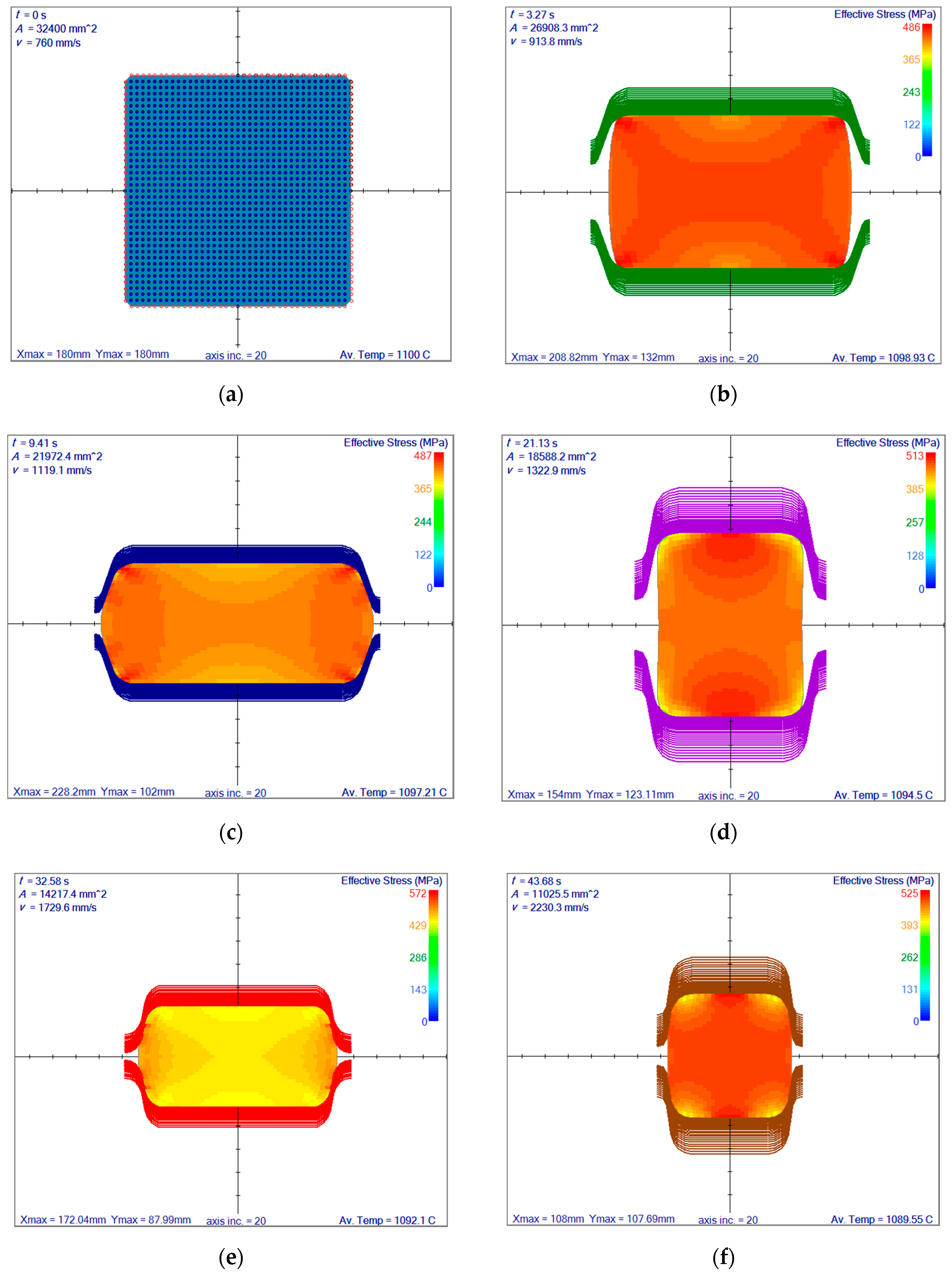
A billet with 180 × 180 mm is chosen to be reverse rolled. Reversing rolling mills, where large deformation rates are applied, are usually considered as a preconditioning rolling stage before the continuous finishing rolling mill. In this section, the strand passes through the same roll with diameter 800 mm back and forth five times and is rotated three times starting from the second pass. The rolling schedule is explicitly as follows. First pass: Forward direction, rotation 0 deg; second pass: Backward direction, rotation 0 deg; third pass: Forward direction, rotation 90 deg; fourth pass: Backward direction, rotation 90 deg; fifth pass: Forward direction, rotation 90 deg. There are 1521 collocation nodes considered, and the results are shown in terms of effective stress in Figure 10. Multiple groove contact lines are drawn starting from the first until the last contact. Each line belongs to one computational step and the amount of reduction may be seen from those lines.
3.4.3. Rotation in between the First and Second Sections
In the first section of reversing rolling mill simulation, the roll has 800 mm diameter. However, in the second section, the roll diameter is 150 mm smaller (650 mm) and the rolling schedule is different. Mostly diamond shape grooves are used, and therefore, the billet is rotated 45 deg at the beginning as demonstrated in Figure 11. For the numerical stability, collocation nodes are redistributed based on ENG algorithm after the rotation as shown in Figure 5b.
3.4.4. Reversing Rolling Mill Simulation–Second Section
This section is the continuation of the first part of the reversing rolling mill. However, in this section, the orientation of the grooves is different than the ones used in the first section. Therefore, the billet is rotated 45 deg before it enters this section, as shown in Figure 11. In between each pass, the billet is again rotated 90 deg with 6 s of rotation time. The rolling schedule is explicitly as follows. Sixth pass: Backward direction, rotation 45 deg; seventh pass: Forward direction, rotation 90 deg; eighth pass: Backward direction, rotation 90 deg; ninth pass: Forward direction, rotation 90 deg; tenth pass: Backward direction, rotation 90°. The strand is rotated back 45 deg at the end of the simulation to observe the final shape. There are 1365 collocation nodes are distributed over the domain after the 45 deg of rotation shown in Figure 11. Effective stress field at each pass may be seen in Figure 12, as well as the final shape, which is 60.55 mm square. A 3 m-long undeformed strand elongates after rolling to 27.37 m.
A sensitivity study based on the temperature field of a slice at the end of the simulation is shown in Figure 13. A comparison of three slice position options, as described in Table 1, is made. The same rolling schedule is considered with the same material properties. Even though the total deformation and time are the same for each simulation, positions of the deformations are different. This leads to a different cooling history and different heat loss at the end for each initial slice position.
4. Discussion
Simulation results in Figure 6, together with many previously compared thermomechanical simulations [16,21,28], show that the novel meshless solution procedure is behaving consistently in comparison with FEM. The deformation is almost the same and temperature interpolation is similar. However, the solution procedure is completely different. The solution procedure differs from FEM in the fact that it is very simple, and it can be straightforwardly extended to 3D, since no geometrical elements are present. An important feature of the presented rolling simulation system is that it is developed by taking into account the needs of the rolling technologists. They may design their own new virtual rolling schedules and optimize them before actual rolling. The initial temperature, material properties, heat transfer coefficients, roll gaps, and groove types may be changed in the simulation. The present research started by developing a flat rolling simulation only. A flat rolling schedule in Figure 7 is simulated, as well as many other flat rolling schedules, by this application. Round schedules are added into the database, and at that moment, it was seen that a node generation algorithm is necessary. ENG is implemented due to its applicability to curved boundaries. For almost all the round and reversing schedules, ENG is used at least once. Here, stability is a big issue, as a large number of collocation nodes usually increase the stability. However, the deformation steps should be reduced with the increased number of the nodes. This substantially increases the computational time.
Different groove types are used in the simulations, but they can be grouped into three categories: Flat, oval, and round. For example, the simulation results shown in Figure 6 took 25 s to complete, the first rolling example took 13 min, and the reversing rolling mill simulation took 51 min to simulate. The highest reduction rates are achieved during the reversing rolling mill simulations. Especially during the first part where the reduction rates are ranging between 38% and 23%. The stress fields in this first part are higher than in the second part where the reduction rates are between 12% and 22%.
The convergence of the LRBFCM with the increase of the number of collocation nodes has been previously demonstrated based on the known analytical solutions [16,28]. The idea here is an efficient simulation system to give the user a complete understanding of what to expect during each roll pass and at the end of the schedule as a final product. A comparison of simulation results with the industrial results has been recently published [17]. There, an error in the schedule design has been simulated and validated by the industrial results. The corrections have been computationally proposed a-priori and a-posteriori approved by defect-free shape. In the simulations, up to 2000 collocation nodes are used for each slice. If the groove has a complex shape, then it is better to increase the number of the collocation nodes, but at the same time, it is necessary to excessively decrease the slice position increments. So, if the user wants to increase the numerical stability, he first needs to reduce the incremental deformation at each time, in other words he needs to reduce the incremental slice movement. Afterwards, he should increase the number of collocation nodes to a higher value. Based on our experience, increasing only the collocation nodes without decreasing incremental slice movement will not lead to more stable results. Otherwise it is not possible to obtain stable results. The least sensitive case is the flat rolling, where the user has a large range of simulation parameters to choose that yield stable results.
The reversing rolling mill simulation capability is added in the present paper, and examples are shown in Figure 10 and Figure 12. ENG is again used here after the second pass and just before the sixth pass. The slice position is chosen as “center” in the simulation results. The total number of computational slices is usually between 1000 and 2000. When there is no contact with the roll surface, only the thermal model is employed, and an incremental slice distance is chosen usually four or five times larger than when there is a contact.
The ongoing research of the authors is microstructure coupling into the macroscale rolling simulation system. The node-based interpolation of the deformation field makes the microstructure implementation easy to handle. For each node, whether the critical strain and time for static or dynamic recrystallization have been reached is checked. Furthermore, empirical grain growth or fractional recrystallization equations are used, and a grain size field may be obtained for each slice. This is another reason why the present meshless method is very suitable for such coupled macro-micro numerical simulation.
5. Conclusions
In this paper, a rolling simulation system, capable of simulating flat, round, and reversing rolling mills is elaborated. Solution procedure is based on meshless LRBFCM, where interpolation of an unknown filed is done through collocation nodes distributed over the computational domain. A slice model assumption is considered to reduce the system of equations to 2D and the solution procedure is repeated for each slice position until the end of rolling. The LRBFCM solution is very simple to implement, since it does not require any background integration like the previous meshless approaches in the field. This simulation system is capable of reading multiple rolling schedules grouped into flat, round, and reverse rolling. The results are shown for a desired slice in terms of displacement vector field, temperature field, effective strain, and effective stress field.
The represented simulation system is developed specifically for hot rolling industrial use. It skips all the time-consuming engineering efforts for creating the geometries and meshing, like in the commercial codes. It is very easy to add new rolling schedules, and the results are usually obtained in less than one hour. The principal use of the system is to a-priori avoid mistakes in the roll pass design. Any user-defined grooves may be implemented, and a systematic sensitivity study of their shapes is obtained very easily. It is shown here that an efficient rolling simulation code may be developed without using any commercial code or library due to the simple implementation of the node-based meshless methods. The simulation system can also be coupled with artificial intelligence [29,30] for automatic optimization with respect to different criteria.
The macro simulation capabilities are in the process of being upgraded to 3D with microstructure models to be able to widen the rolling analysis and to have a better understanding of the final product’s microstructure and properties.
Author Contributions
B.Š. provided “Conceptualization and Methodology”, U.H. provided “Software Development and Validation”.
Funding
This research was funded by Slovenian Grant Agency, grant numbers P2-0162 and L2-9246 and Štore-Steel Company (www.store-steel.si).
Conflicts of Interest
The authors declare no conflict of interest. The funders had no role in the design of the study; in the collection, analyses, or interpretation of data; in the writing of the manuscript, and in the decision to publish the results.
Appendix A
| Heat transfer coefficient to air | hair | 20 | W/m2·K |
| Heat transfer coefficient to roll | hroll | 10,000 | W/m2·K |
| Thermal conductivity of steel | λ | 29 | W/m2·K |
| Specific heat of steel | cp | 630 | J/kg·K |
| Initial rolling speed | ventry | 0.76 | m/s |
| Ambient temperature | Tair | 25 | °C |
| Roll surface temperature | Troll | 500 | °C |
| Initial slice temperature | Tinitial | 1100 | °C |
| Taylor-Quinney parameter | η | 0.9 | - |
| Time step | Δt | 10−4 | s |
| Coefficient of friction | μ | 0.1 | - |
| Material model | Mpa | ||
| Distance between rolling stands | - | 3 (for the first five rolling stands), 4.5 (after fifth rolling stand) | m |
| Exit distance of the billet in reversing rolling mill | - | 1 | m |
References
- Lenard, J.G.; Pietrzyk, M.; Ceser, L. Mathematical and Physical Simulation of the Properties of Hot Rolled Products, 1st ed.; Elsevier: Oxford, UK, 1999. [Google Scholar]
- Roberts, W.L. Cold Rolling of Steel; Marcel Dekker Inc.: New York, NY, USA, 1978. [Google Scholar]
- Roberts, W.L. Hot Rolling of Steel; Marcel Dekker Inc.: New York, NY, USA, 1983. [Google Scholar]
- Sims, R.B. The calculation of the roll force and torques in hot rolling mills. Proc. Inst. Mech. Eng. 1954, 168, 191–200. [Google Scholar] [CrossRef]
- Wusatowski, Z. Hot rolling: A study of drought, spread and elongation. Iron Steel 1955, 28, 49–54. [Google Scholar]
- Gallagher, R.H. Stress analysis of heated complex shapes. J. Am. Rocket Soc. 1962, 32, 700–707. [Google Scholar] [CrossRef]
- Marcel, P.V.; King, L.P. Elastic-plastic analysis of two-dimensional stress systems by the finite element method. IJMS 1967, 9, 143–155. [Google Scholar] [CrossRef]
- Mori, K.; Osakada, K.; Oda, T. Simulation of plane-strain rolling by the rigid plastic finite element method. Int. J. Mech. Sci. 1982, 24, 519–527. [Google Scholar] [CrossRef]
- Glowacki, M.; Kedzierski, Z.; Kusiak, H.; Madej, M.; Pietrzyk, M. Simulation of metal flow, heat transfer and structure evolution during hot rolling in square-oval-square series. J. Mater. Process. Technol. 1992, 34, 509–516. [Google Scholar] [CrossRef]
- Kikuma, T.; Yamada, K. Progress of Finite Element Simulation for Rolling Processes. In Proceedings of the 7th International Conference on Numerical Methods in Industrial Forming Process, Toyohashi, Japan, 18–20 June 2001. [Google Scholar]
- Belytschko, T.; Lu, Y.Y.; Gu, L. Element-free Galerkin methods. Int. J. Numer. Methods. Eng. 1994, 37, 229–256. [Google Scholar] [CrossRef]
- Onate, E.; Idelsohn, S.; Zienkiewicz, O.C.; Taylor, R.L. A finite point method in computational mechanics. Int. J. Numer. Methods. Eng. 1996, 39, 3839–3866. [Google Scholar] [CrossRef]
- Atluri, S.N.; Zhu, T. A new meshless local Petrov-Galerkin approach in computational mechanics. Comput. Mech. 1998, 22, 117–127. [Google Scholar] [CrossRef]
- Chen, Y.; Lee, J.D.; Eskandarian, A. Meshless Methods in Solid Mechanics; Springer: New York, NY, USA, 2006. [Google Scholar]
- Cueto, E.; Chinesta, F. Meshless methods to the simulation of material forming. Int. J. Mater. Form. 2013, 8, 25–43. [Google Scholar] [CrossRef]
- Hanoglu, U.; Šarler, B. Simulation of hot shape rolling of steel in continuous rolling mill by local radial basis function collocation method. Comp. Model. Eng. 2015, 109, 447–479. [Google Scholar] [CrossRef]
- Hanoglu, U.; Šarler, B. Rolling simulation system for non-symmetric groove types. Procedia Manuf. 2018, 15, 121–128. [Google Scholar] [CrossRef]
- Vertnik, R.; Mramor, K.; Šarler, B. Solution of three-dimensional temperature and turbulent velocity field in continuously cast steel billets with electromagnetic stirring by a meshless method. Eng. Anal. Bound. Elem. 2019, 104, 347–363. [Google Scholar] [CrossRef]
- Mavrič, B.; Šarler, B. Local radial basis function collocation method for linear thermoelasticity in two dimensions. Int. J. Numer. Method H. 2015, 25, 1488–1510. [Google Scholar] [CrossRef]
- Lenard, J.G. Primer on Flat Rolling, 1st ed.; Elsevier: Oxford, UK, 2017. [Google Scholar]
- Hanoglu, U.; Šarler, B. Thermo-mechanical analysis of hot shape rolling of steel by a meshless method. Procedia Eng. 2011, 10, 3173–3178. [Google Scholar] [CrossRef]
- Hanoglu, U.; Šarler, B. Multi-pass hot rolling simulation using a meshless method. Comput. Struct. 2018, 194, 1–14. [Google Scholar] [CrossRef]
- Chen, W.F.; Han, D.J. Plasticity for Structural Engineers; Springer: New York, NY, USA, 1988. [Google Scholar]
- Vertnik, R.; Šarler, B. Meshfree local radial basis function collocation method for diffusion problems. Comput. Math. Appl. 2006, 51, 1269–1282. [Google Scholar] [CrossRef]
- Kobayashi, S.; Oh, S.; Altan, T. Metal Forming and Finite Element Method; Oxford University Press: New York, NY, USA, 1989. [Google Scholar]
- Thompson, A.J.F.; Soni, B.K.; Weatherill, N.P. Handbook of Grid Generation; CRC: Tallahassee, FL, USA, 1999. [Google Scholar]
- DEFORM 2D, Scientific forming technologies corporation, Version 10.1. 2009. Available online: http://www.deform.com (accessed on 23 May 2019).
- Hanoglu, U. Simulation of Hot Shape Rolling of Steel by a Meshless Method. Ph.D. Thesis, University of Nova Gorica, Nova Gorica, Slovenia, 2015. [Google Scholar]
- Kovačič, M.; Šarler, B. Genetic programming prediction of the natural gas consumption in a steel plant. Energy 2014, 66, 273–284. [Google Scholar] [CrossRef]
- Kovačič, M.; Stopar, K.; Vertnik, R.; Šarler, B. Comprehensive electric arc furnace electric energy consumption modeling: A pilot study. Energies 2019, 12, 2142. [Google Scholar] [CrossRef]
Figure 1.
Different types of rolls: (a) flat, (b) round, and (c) non-symmetric.

Figure 2.
Scheme of the slice model and rolling layout. Area A, time t, position z, and velocity v, are calculated for each slice.
Figure 2.
Scheme of the slice model and rolling layout. Area A, time t, position z, and velocity v, are calculated for each slice.

Figure 3.
Domain and boundary discretization example with local influence domains consisting of five or seven nodes.
Figure 3.
Domain and boundary discretization example with local influence domains consisting of five or seven nodes.

Figure 4.
Direct iteration procedure.

Figure 5.
(a) Regular vs. (b) ENG node distribution.

Figure 6.
(a) Local Radial Basis Function Collocation Method (LRBFM) result vs. Finite Element Method (FEM) result when there is no heat flux at the boundaries, uniform temperature filed at the beginning. The increase in temperature is achieved by internal heat generation due to plastic deformation. Initial size: 126 × 81 mm, compressed to 65 mm height. (b) The comparison of final shapes after the deformation. Effective strain fields are calculated by LRBFCM (c) and FEM (d).


Figure 7.
Flat rolling simulation results in terms of effective strain fields. (a) Initial size, (b) after first pass, (c) after second pass, (d) after third pass, (e) after fourth pass, (f) after fifth pass, (g) after sixth pass, (h) after seventh pass, (i) after eighth pass.
Figure 7.
Flat rolling simulation results in terms of effective strain fields. (a) Initial size, (b) after first pass, (c) after second pass, (d) after third pass, (e) after fourth pass, (f) after fifth pass, (g) after sixth pass, (h) after seventh pass, (i) after eighth pass.


Figure 8.
Simulation results calculated at each pass in terms of (a) maximum effective strain, (b) maximum effective stress. The increasing effect of the coefficient of friction is seen toward the end of the rolling schedule.
Figure 8.
Simulation results calculated at each pass in terms of (a) maximum effective strain, (b) maximum effective stress. The increasing effect of the coefficient of friction is seen toward the end of the rolling schedule.


Figure 9.
Oval rolling simulation results in terms of displacement fields. (a) After first pass, (b) after second pass, (c) after third pass, (d) after fourth pass, (e) after fifth pass, (f) after sixth pass, (g) after seventh pass.
Figure 9.
Oval rolling simulation results in terms of displacement fields. (a) After first pass, (b) after second pass, (c) after third pass, (d) after fourth pass, (e) after fifth pass, (f) after sixth pass, (g) after seventh pass.


Figure 10.
Reversing rolling mill simulation where the billet is rotated 90 degrees after each pass, starting from the second pass and 6 s of rotation time is considered. Results are shown in terms of effective stress field. (a) Initial size, (b) after first pass, (c) after second pass, (d) after third pass, (e) after fourth pass, (f) after fifth pass.

Figure 11.
Rotation of 45 degrees before the second part of the reversing rolling simulations.

Figure 12.
Second part of the reversing rolling mill simulation, where the roll diameter used is 650 mm before and after the billet is rotated 45 deg. In between the passes, it is rotated 90 deg. Results are shown in terms of effective stress filed. (a) After sixth pass, (b) after seventh pass, (c) after eighth pass, (d) after ninth pass, (e) after tenth pass, (f) final shape with temperature field.


Figure 13.
Temperature filed comparisons at the end of the reversing rolling simulation. Different initial slice positions are chosen and compared.
Figure 13.
Temperature filed comparisons at the end of the reversing rolling simulation. Different initial slice positions are chosen and compared.


Table 1.
Demonstration of computational slice positions during reversing rolling mill simulation.
| Head | Centre | End |
|---|---|---|
| Initial slice | Initial Slice | Initial Slice |
 |  |  |
| First roll | First roll | First roll |
 |  |  |
| Second roll | Second roll | Second roll |
 |  |  |
© 2019 by the authors. Licensee MDPI, Basel, Switzerland. This article is an open access article distributed under the terms and conditions of the Creative Commons Attribution (CC BY) license (http://creativecommons.org/licenses/by/4.0/).
Share and Cite
MDPI and ACS Style
Hanoglu, U.; Šarler, B. Hot Rolling Simulation System for Steel Based on Advanced Meshless Solution. Metals 2019, 9, 788. https://doi.org/10.3390/met9070788
AMA Style
Hanoglu U, Šarler B. Hot Rolling Simulation System for Steel Based on Advanced Meshless Solution. Metals. 2019; 9(7):788. https://doi.org/10.3390/met9070788
Chicago/Turabian StyleHanoglu, Umut, and Božidar Šarler. 2019. "Hot Rolling Simulation System for Steel Based on Advanced Meshless Solution" Metals 9, no. 7: 788. https://doi.org/10.3390/met9070788
Note that from the first issue of 2016, this journal uses article numbers instead of page numbers. See further details here.