Parametric Robust Control of the Multivariable 2 × 2 Looper System in Steel Hot Rolling: A Comparison between Multivariable QFT and H_∞

Abstract

Two robust mutlivariable controllers, H_∞ and a decentralized quantitative feedback theory (QFT), are designed in the frequency domain for the 2 × 2 looper system in a steel hot rolling mill to keep stability in the presence of parametric uncertainties. The H_∞ controller is designed by using the mixed sensitivity approach, while the multivariable decentralized QFT is designed by the extension of the sequential loop closing method presented elsewhere. Stability robustness conditions are verified in the frequency domain, while simulations in time domain are carried out to evaluate the controllers and compare their performance along with that of proportional + integral (PI) and single input single output (SISO) QFT controllers designed earlier. The QFT controller shows the best balance among the performance indicators analyzed here; however, at the expenses of using higher power in one of the control inputs.

1. Introduction

A hot strip mill (HSM) is a process that rolls steel slabs into coiled strips. The finishing mill (FM), where the strip takes the final thickness, is the most critical process in an HSM because of the great number of variables involved, interactions between them, and hence its modeling complexity and uncertainty [1,2]. On the other hand, as with many other industrial processes, the environment is highly noisy.

The FM has to attain desired strip thickness and finishing temperature, therefore, controlling these variables and those that have an impact on them is highly important. Most FMs are controlled by proportional + integral (PI) control strategies, which are not designed to compensate for the above-mentioned difficulties. During the past two decades, control of relevant aspects related to thickness has been an active research topic in the literature [3,4,5,6,7,8]. Special attention has been paid to the looper system variables, tension and looper angular position, owing mainly to their great influence on strip thickness and finishing temperature [2]. Several control approaches for these variables with the aim of achieving stability and performance in the presence of uncertainties and interactions have been proposed.

H_∞ control schemes were proposed for thickness and mass flow loops to achieve robustness in the presence of sensor failures [9]. A 2 × 2 multivariable robust parametric H_∞ controller was designed for thickness and looper angular position [10]. Two H_∞ robust controllers for strip tension were presented; one of them designed using Lyapunov–Krasovskii method and LMIs and the other by the conventional 2-Riccati-equation based method [11]. Chen et al. proposed a discrete-time H_∞ robust controller [12]; while a two nested closed loop scheme, a decoupling decentralized control and an H_∞ robust controller, was presented in [13].

Hearns and Grimble [14] proposed an inferential control designed by the quantitative feedback theory (QFT) technique for strip tension control. The same authors [15] have presented a control based on QFT technique for the looper system, however, the standard approach found in the literature [16,17] was modified for that particular application.

Two single loop QFT parametric robust controllers for strip tension and looper angular position were designed [18]. Tests under parametric uncertainty have been conducted within a 2 × 2 scheme of the looper system, comparison with conventional PI controllers have also been carried out. A single loop parametric robust QFT controller for strip thickness was also designed [19]. It was also tested in a 2 × 2 scheme together with the looper angular position presented in [18] and performance was compared with that of PI controllers.

Although the present work is concerned with those techniques using a fixed linear robust controller in the frequency domain, it is worth mentioning that model based predictive controllers (MPC) [20,21,22,23] as well as non-linear techniques [24,25] have been applied to the looper system.

As shown by the above survey, there is as great concern about achieving robustness and interaction rejection for the looper system in an HSM by H_∞ and QFT control design techniques. Hence, anticipating potential applications on an actual HSM, it would be worthwhile to evaluate the techniques and compare their performance using controllers designed by standard approaches commercially available in control design software tools such as MATLAB. Thus, in this work, two multivariable parametric robust controllers are designed, QFT and H_∞, for the multivariable 2 × 2 looper system. As far as the author knowledge is concerned, MIMO QFT controllers have not been applied to the looper system in an HSM. The QFT controller is designed by the decentralized QFT control technique for multivariable processes (mvQFT) as given in Yaniv [26] using the MATLAB/QFT toolbox; while the H_∞ controller was designed by the mixed sensitivity approach and the standard 2-Riccati-equation solution using the MATLAB HINF function. The controllers are also compared with PI controllers, which are the current controllers in most HSMs worldwide, and the two SISO QFT controllers presented in [18], when applicable; evaluating in this way, the potential benefits of compensating for interactions and parameter uncertainty. The multivariable linearized HSM model presented and experimentally validated in Obregon et al. [2] has been built in Simulink to perform time domain tests.

The paper is organized as follows. Section 2 describes briefly the model used in this work. Section 3 presents the fundamentals of the QFT and H_∞ control techniques. Section 4 deals with the controllers designed for the looper system. In Section 5 the simulation results are presented and discussed, and finally, Section 6 presents the conclusions.

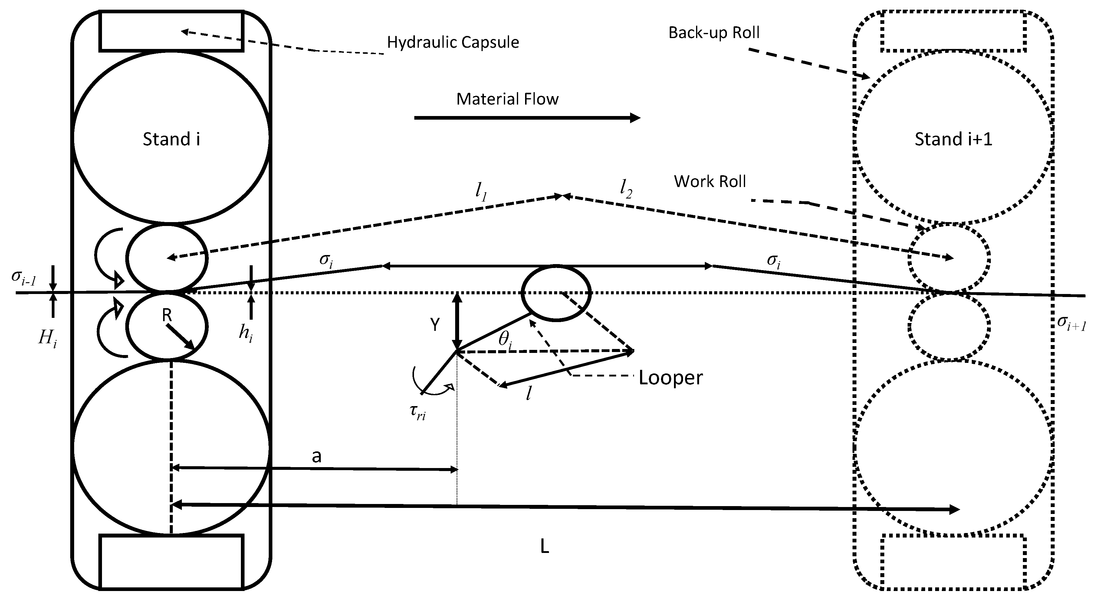
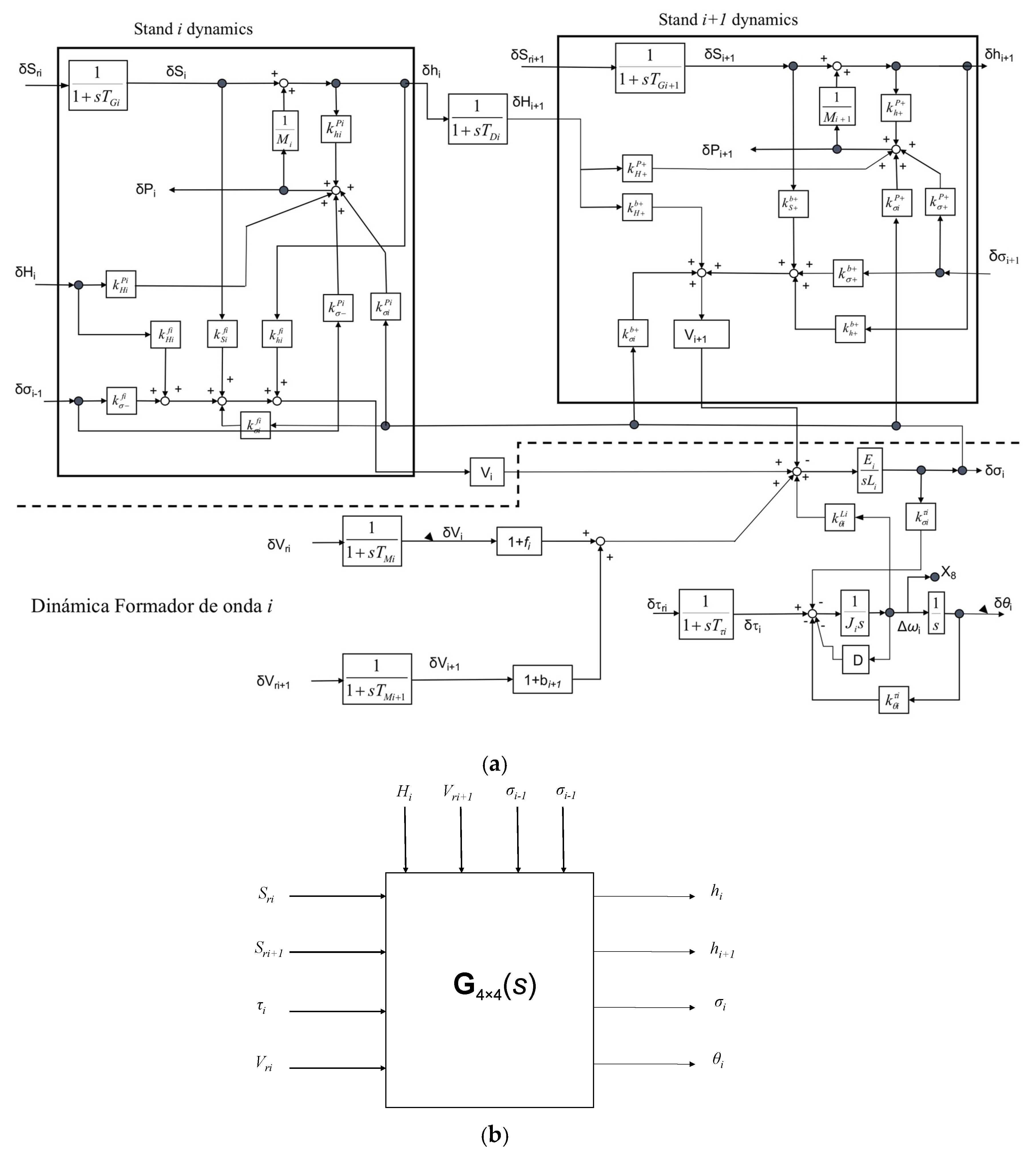
2. FM Multivariable Model

Two FM contiguous stands, i and i + 1, and the lopper i between them were represented by a linear 4 × 4 multivariable model [2]. The assumption of a linear behavior is realistic, since the mill operates under small signal regime once the steel bar has been threaded.

Figure 1 is a schematic representation of the two modeled stands, while the model block diagram is shown in Figure 2a. To validate the model, it was built in Simulink and tests were performed with data from the real mill, concluding that it was a good approximation of the process [2]. To derive the model some blocks were represented directly in Laplace while the nonlinear static relations involved were linearized around an operating point. The operating conditions were defined according to the rolling practice of the most commonly rolled product in stands 3 (i) and 4 (i + 1). In Figure 2a, δ denotes small perturbation; the symbol $K_x^y$ denotes a static gain obtained from linearization, this being $\frac{\partial y}{\partial x}$ evaluated at the operating conditions; a plus symbol (+) or a minus symbol (−), on either the superscript or the subscript of $K_x^y$ denote i + 1 and i − 1 stands respectively. The symbology is shown in

Table 1. Variables and physical parameters.

Variable	Symbol	Units	Parameter	Symbol	Units
Stand i hydraulic cylinder position reference	Sri	m	Stand i mill modulus	Mi	N/m
Stand i + 1 hydraulic cylinder position reference	Sri+1	m	Stand i + 1 mill modulus	Mi+1	N/m
Stand i roll linear velocity reference	Vri	m/s	Steel Young’s modulus at operating temperature	Ei	N/m2
Looper i torque reference	τi	Nm	Looper i roll radius	r	m
Stand i exit thickness	hi	m	Distance between stand i and i + 1 backup roll centers	Li	m
Stand i entry thickness	Hi	m	Steel density	ρ	Kg/m3
Stand i + 1 exit thickness	hi+1	m	Looper i momentum of inertia	Ji	Kgm2
Stand i − 1 exit tension	σi−1	N	Looper i friction	Di	Nm/rad/s
Stand i roll linear velocity	Vi	m/s	Stand i cylinder position regulator time constant	TGi	s
Stand i + 1 roll linear velocity reference	Vri+1	m/s	Stand i + 1cylinder position regulator time constant	TGi+1	s
Stand i exit tension	σi	N	Time constant of delay approximation between hi y Hi+1	TDi	s
Stand i + 1 exit thickness	σi+1	N	Stand i work roll speed regulator time constant	TMi	s
Looper i length	li	m	Stand i + 1 work roll speed regulator time constant	TMi+1	s
Looper i angular position	θi	Radians	Looper i torque regulator time constant	Tτi	s
Stand i roll separation force	Pi	N	Stand i forward slip	fi	-
Stand i + 1 roll separation force stand i + 1	Pi+1	N	Stand i + 1 backward slip	bi+1	-

.

The four model outputs are: (1) stand i exit strip thickness (h_i), (2) stand i + 1 exit strip thickness (h_i+1), (3) strip tension (σ_i), and (4) looper i angular position (θ_i). Their corresponding control inputs according to the conventional coupling are: (1) position reference for stand i hydraulic cylinder (S_ri), (2) position reference for stand i + 1 hydraulic cylinder (S_ri+1), (3) torque reference for looper i motor (τ_ri), and (4) speed reference for stand i motor (V_ri). The stand i input thickness (H_i), the speed reference for stand i + 1 motor (V_ri+1), the stand i − 1 tension (σ_i−1), and the stand i + 1 tension (σ_i+1) are considered to be perturbations. A remark is worthwhile here, although V_ri+1 is the drive speed reference for the stand i + 1 motor, it is the control input for θ_i+1 controlled by the upstream controller; however, it may cause variations on σ_i, acting as a perturbation for the looper i controller. Figure 2b shows the model representation in one block.

In this work, two robust controllers for the 2 × 2 looper system will be designed. The reduced 2 × 2 plant is a 5th order matrix transfer function (TFM) with one pair of complex poles. The TFM G(s) of the linearized system is given by:

$$\left[\begin{array}{c}{\sigma }_i\\ {\theta }_i\end{array}\right]=\mathbf{G}\left(s\right)\left[\begin{array}{c}{\tau }_i\\ V_{ri}\end{array}\right],$$

(1)

where

$\mathbf{G}\left(s\right)=\left[\begin{array}{cc}{g}_{11}\left(s\right)& g_{12}\left(s\right)\\ g_{21}\left(s\right)& g_{22}\left(s\right)\end{array}\right]$ and

$$\begin{gathered} g_{11}\left(s\right)=\frac{-107.8s^2-52.83s}{s^5+9.129s^4+1939s^3+1.124\times {10}^4{s}^2+8495s+1336} \\ {g}_{21}\left(s\right)=\frac{12.12s^2+49.4s+16.45}{s^5+9.129s^4+1939s^3+1.124\times {10}^4{s}^2+8495s+1336} \\ {g}_{12}\left(s\right)=\frac{81.59s^3+44.32s^2+1.606\times {10}^{4}s+7873}{s^5+9.129s^4+1939s^3+1.124\times {10}^4{s}^2+8495s+1336} \\ {g}_{22}\left(s\right)=\frac{1.578\times {10}^{4}s-7737}{s^5+9.129s^4+1939s^3+1.124\times {10}^4{s}^2+8495s+1336} \end{gathered}$$

Six parameters are considered to be uncertain, owing to the huge complexities involved on the parameter uncertainty identification, being generally subject to measurement uncertainties and noise, the uncertainty regions will be assumed to have a given size depending on each parameter as explained below.

A large uncertainty was assumed to be of ±20% around the operating value. This was assigned to two physical parameters E_i and D due to the following reasons. In [2], E_i was taken from the ASM manual [27], however, only values up to 400 °C are provided. The strip temperature between stands 3 and 4 in the HSM of study is approximately 800 °C, E_i value was extrapolated by using the slope between the last two points provided. Notwithstanding, since E_i decreases more rapidly above 400 °C [27], the slope should be steeper and hence a large uncertainty was assumed. On the other hand, D was experimentally tuned, assuming as well to have a large uncertainty. J_i was calculated from the looper geometry and it was considered to have a medium size uncertainty of ±10%. The gains $K_{{\theta }_i}^{L_i}$, $K_{{\sigma }_i}^{{\tau }_i}$, and $K_{{\theta }_i}^{{\tau }_i}$ were calculated from linearization of well-established nonlinear relations as well as rolling practices long-accepted in the real-life mills; therefore, they were considered to be bounded within a small uncertainty region of ±5%.

Figure 3a shows the largest and the smallest singular values in the frequency domain of the TFM G(s), denoted by $\overline{\sigma }\left(\mathbf{G}\left(s\right)\right)$ and $\underset{\_}{\sigma }\left(\mathbf{G}\left(s\right)\right)$ respectively. $\overline{\sigma }\left(\mathbf{G}\left(s\right)\right)$ and $\underset{\_}{\sigma }\left(\mathbf{G}\left(s\right)\right)$ are the largest and smallest possible gains for all input directions at each frequency. Five values uniformly distributed within each parameter uncertainty region were considered; given the six uncertain parameters aforementioned 5⁶ different plants are obtained. Figure 3b shows $\overline{\sigma }$ for all the 5⁶ plants. It can be seen that the largest behavior deviation is between 30 and 70 rad/s.

3. Methodology

3.1. Multivariable Decentralized Robust QFT Controller

The QFT robust control technique was originally proposed for single-input single-output (SISO) systems and it is aimed to keep stability and performance in the presence of parametric uncertainties [16,17]. The parametric uncertainty is modeled as a set of plants {∏} in which every particular plant G(s)∈∏ is generated by a given set of parameter values.

A finite and sufficiently large number of plants G(s)∈∏ is plotted in the frequency domain by using the Nichols chart for some determined working frequencies. A collection of points represents the frequency response of the plotted plants at any given working frequency. The outer points delimit an uncertainty area on the Nichols chart called “templates”. Considering the two-degrees of freedom unity feedback closed loop scheme of Figure 4, assuming the scalar case, the closed loop transfer function can be expressed as:

$$T\left(s\right)=\frac{G\left(s\right)K\left(s\right)}{1+G\left(s\right)K\left(s\right)}F\left(s\right)$$

where K(s) and F(s) are the controller and the prefilter transfer functions respectively, and T(s) should remain stable for all G(s)∈∏.

The closed loop system should also satisfy the following conditions:

• for tracking specifications:

  $$a\left(\omega \right)\le \left|T\left(j\omega \right)\right|\le b\left(\omega \right),\forall \omega \mathrm{and}G(\mathrm{s})\in \prod$$

  (2)

  where 0 ≤ |a(ω)|< |b(ω)| ∀ ω.
• and for disturbance rejection specifications:

  $$\left|S\left(j\omega \right)\right|\le d\left(\omega \right),\forall \omega \mathrm{and}G(\mathrm{s})\in \prod$$

  (3)

  where S is the sensitivity function to output disturbances.

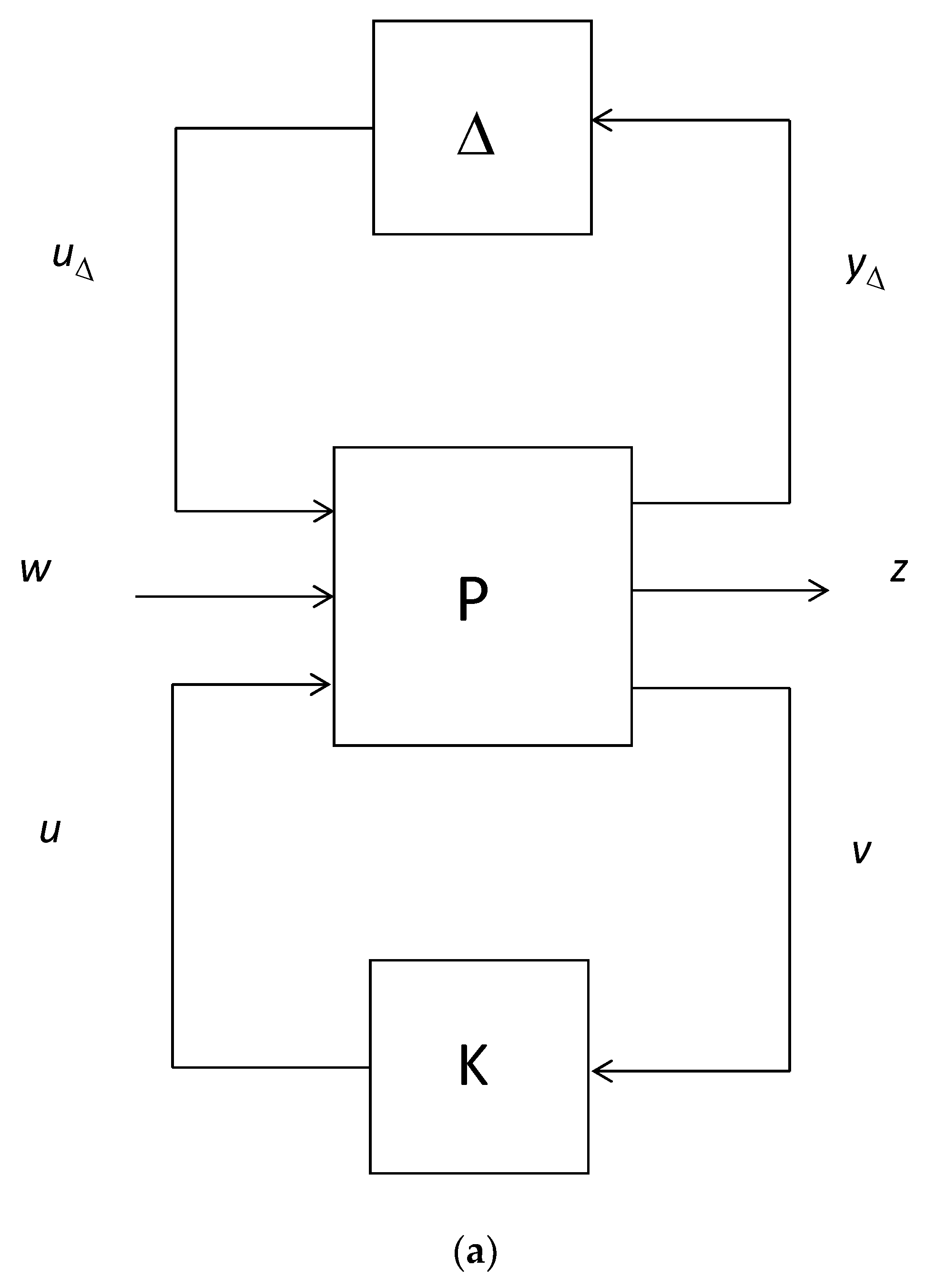
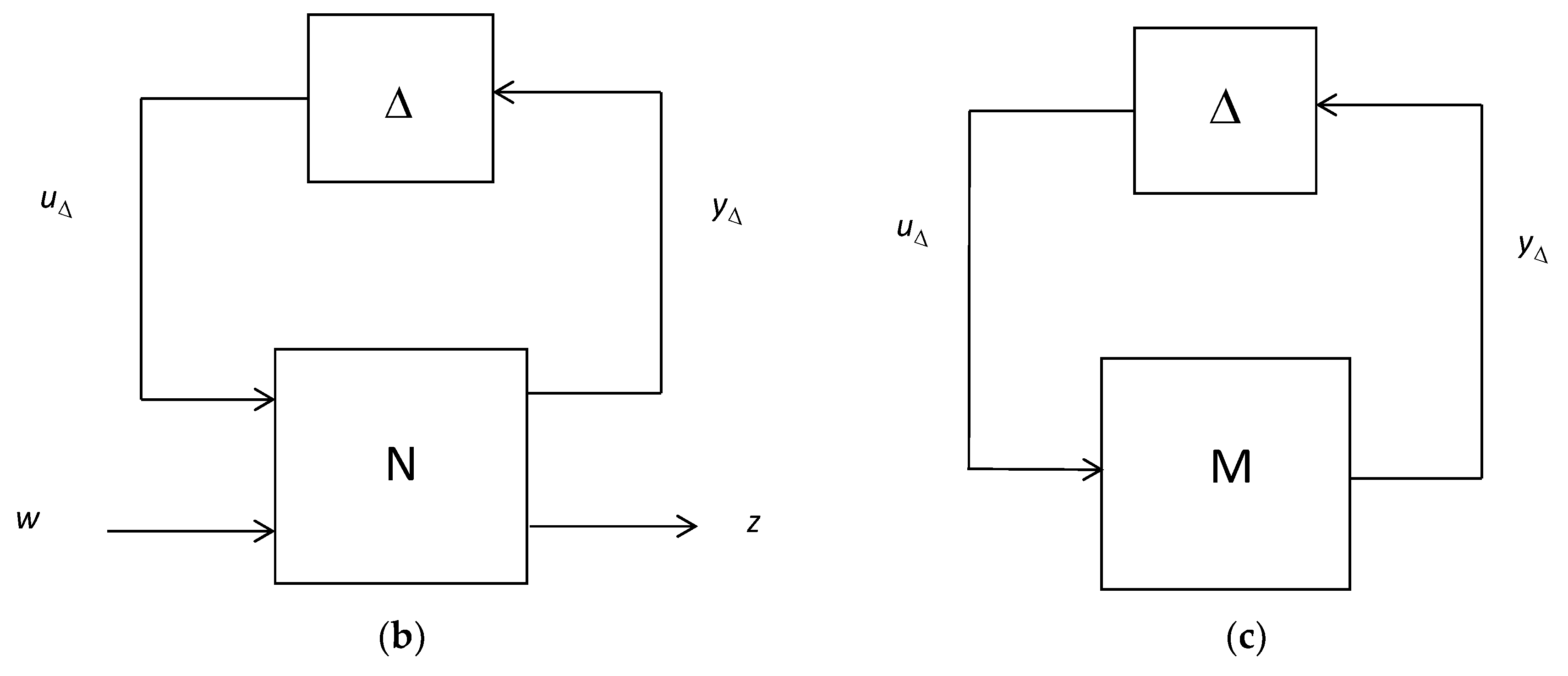
A nominal plant G₀(s)∈∏ is arbitrarily chosen, then, by using the so-called M-circles, specification boundaries are obtained for the nominal open loop (L₀(jω)) at each working frequency. The controller K(s) is designed by loopshaping such that the nominal plant is above the boundaries; however, the technique ensures all the possible open loops conformed by K(s) and all the plants within the template (L(jω)) fulfill conditions given in Equations (1) and (2).

For an n × n multi-input multi-output (MIMO) system, assuming a diagonal controller, the problem was replaced by n × n single loops [16,17]. The method was further developed using iteratively the sequential loop closing technique [26]. In this work, this method is used to design a decentralized mvQFT controller for the looper system.

Given a multivariable two-degrees of freedom closed loop scheme (Figure 4) with G∈∏ the plant TFM, ∏ the set of uncertain MIMO plants, and K and F the controller and prefilter TFMs respectively, the complementary sensitivity TFM is given by:

$$T=GK{(I+GK)}^{-1}F,$$

(4)

should remain stable ∀ G∈∏.

Assuming a square n × n plant G, the conditions given in Equations (1) and (2) are extended for multivariable systems as follows:

$$a_{ij}\left(\omega \right)\le \left|t_{ij}\left(j\omega \right)\right|\le b_{ij}\left(\omega \right),\forall \omega \mathrm{and}\mathbf{G}\left(\mathrm{s}\right)\in \mathbf{\prod },$$

(5)

and

$$\left|1+L_i^n\right|\ge D_i\left(\omega \right),\forall \omega \mathrm{and}\mathbf{G}\left(\mathrm{s}\right)\in \mathbf{\prod },$$

(6)

where i = 1, …, n, j = 1, …, n, t_ij is the (i, j) element of T, and Lⁿ_i is the i-loop transfer when only the i-loop is open.

It has been shown that by using the sequential loop closing method, condition (5) is fulfilled, and for condition (6) to be satisfied, the recursive procedure proposed in [26] is sufficient. Such procedure was used in this work.

3.2. H_∞ Robust Controller

The H_∞ controller is designed by the mixed-sensitivity approach, which is based on the general control problem scheme depicted in Figure 5a. The general control problem scheme is built from the conventional control scheme given in Figure 4, assuming F = I. In Figure 5a, w represents the external inputs, z is the output vector with the functions to be minimized, P is the generalized or augmented plant TFM, K is the controller TFM and Δ is a block diagonal matrix representing the uncertainties with ‖Δ‖_∞≤1. Assuming again a square n × n MIMO plant G(s), the dimensions of P are multiples of n. The structure of P greatly depends on the particular control problem definition, a typical definition would be as follows. w and z are usually taken as w = [r d]^T and z = [e u y]^T, since r, d, e, u and y, are all vectors of dimension n, w is a vector of dimension 2n and z is a vector of dimension 3n. Note that u is the plant (G) input and it might be, as in this case, both, input and output of P, see Figure 4 and Figure 5a. On the other hand, v is the controller (K) input, which is e, hence it is a vector of dimension n. Now assuming q sources of uncertainties, u_Δ and y_Δ are vectors of dimension qn. With this considerations, P would be a matrix of (q + 3 + 1)n × (q + 2 + 1)n. P, in general, is an array of n × n blocks expressed in terms of G, 0_n×n or I_n×n, depending on the particular input/output relations [28].

The problem is to find a controller that minimizes the H_∞ norm of the closed-loop transfer function from w to z. For analysis purposes the controller can be incorporated and the scheme shown in Figure 5b is obtained. The closed loop transfer function is given by:

$$F_{zw}\left(N,\mathsf{\Delta }\right)=N_{22}+N_{21}\mathsf{\Delta }{(I-N_{11}\mathsf{\Delta })}^{-1}{N}_{12},$$

(7)

For stable nominal open loop system and Δ, the only source of instability in Equation (10) is the term (I-N₁₁Δ)⁻¹, therefore, for robust stability in the presence of unstructured uncertainties, it is sufficient to analyzed the so-called “M-Δ structure” with M = N₁₁, and depicted in Figure 5c.The condition for robust stability in the presence of unstructured uncertainties [28] is given by:

‖M‖_∞<1 with ‖Δ‖_∞≤1,

(8)

In this work, the parametric uncertainty will be represented by an unstructured output multiplicative uncertainty, then Equation (8) becomes:

‖W₁TW₂‖_∞<1 with ‖Δ‖_∞≤1,

(9)

where W₁ and W₂ are the uncertainty weights.

The H_∞ mixed-sensitivity problem is to find a controller such that:

$${\Vert \begin{array}{c}{W}_{P}S\\ W_{U}KS\\ W_{T}T\end{array}\Vert }_{\infty }<1,$$

(10)

with W₂ = I and W₁ = W_T, W_P is the nominal performance specification and W_U is the plant input weight.

4. Controller Designed

The controllers will be designed to attain stability in the presence of parametric uncertainties for the 2 × 2 looper system assuming null inputs on S_ri and S_ri+1, see Figure 2b; note that the feedback blocks from σ_i to V_i are still taken into account, see Figure 2a. Six parameters will be considered to be uncertain, as mentioned in Section 2, however, bounded within a region around the parameter operating value. It is worth noting that the design methods used here assume uncertain time-invariant parameters.

The QFT technique models the parametric uncertainty in the frequency domain; hence, to allow a straight comparison, the parametric uncertainty will be modeled in the frequency domain as well for the H_∞ controller design. On the other hand, the controllers will be designed separately searching for the best performance that can possibly be achieved with each technique.

In this work, as in most works on looper control, it is assumed that tension measurement is available, even though it is not usually the case [21,25]. Nonetheless, the parametric uncertainty as modeled here, the plant templates in QFT and a diagonal output multiplicative uncertainty in H_∞ compensate, until certain extent, for the uncertainties introduced by the lack of tension measurements [14,27,29]; representing this a progress with respect to the currents controllers (PI) in the actual mills. Further study on this topic is left for future work.

4.1. mvQFT Robust Controller Design for the Looper System

As mentioned, QFT is a frequency domain design technique based on Nichols charts. The design procedure is iterative, and it is usually given in five steps.

Step #1. Specification definition.

The stability robustness specifications are given as follows:

0 ≤ t₁₁ ≤ 2 and 0 ≤ t₂₂ ≤ 1.9,

(11)

While the performance specifications that produced the best results given in terms of S were the following:

$$S\left(s\right)\le \left[\begin{array}{cc}0.03\frac{s^3+64s^2+748s+2400}{s^2+14.4s+169}& 0.75\\ 5.2& 0.045\frac{s^3+64s^2+748s+2400}{s^2+14.4s+169}\end{array}\right],$$

(12)

Note that Equation (6) may be obtained from Equation (12).

Step #2. Template generation.

The working frequencies are first selected to plot the frequency response of g^l_uu(jω), which is the diagonal element of G^l∈∏, where G^l is is a square TFM as assumed in [26], l is a finite integer (1, 2, 3, …, v) denoting a given set of parameter values, see Section 2 and Figure 3b, and v is the total number of sets. This method does not guaranty the worst-case plant to be included; hence it was decided to use an exhaustive number of sets. As mentioned, five values uniformly distributed within each parameter uncertainty region were considered; given the six uncertain parameters aforementioned, v is equal to 5⁶. Therefore, a template is the plot of 15,625 points, corresponding each to every particular G^l∈∏ at any given working frequency. Only the templates for g^l_uu(jω) are needed, hence, for the sake of briefness, the plots are not shown here, however they can be found in [18], where it can be seen that the largest templates, meaning the largest uncertainty regions are consistent with Figure 3b. Since the procedure is iterative, the working frequencies were readjusted, the final selected working frequencies in rad/s were: 0.1, 2, 7, 36, 43, 45, 68, 105, 1000, and 3000.

Step #3. Specification boundaries generation.

The specifications boundaries for stability robustness and disturbance rejection are generated in this step; global boundaries are obtained, which are the union of all the particular boundaries for every specification at every working frequency. They are shown in Figure 6, for the sake of briefness they are shown along with L_0u (u = 1, 2, in this case) designed in the next step.

Step #4. Controller Design.

The controller has been designed by loop-shaping in the Nichols Chart by adding poles and/or zeros such that the close-loop system is stable and L₀ is above the specification boundaries at each frequency. In this step the recursive design procedure, mentioned in Section 3.1 and given in [26], is executed assuming F = I. L₀₁ and L₀₂ for the final design are shown in Figure 6.

Step #5. Specification fulfillment verification.

Specification fulfillment is verified in the frequency domain. In Figure 7a,b plots of |t_ii(jω)| and |s_ij(jω)| are shown. As can be seen in the plots, the specifications are met.

4.2. H_∞ Robust Controller Design for the Looper System

As mentioned, since the mvQFT technique models the parametric uncertainty in the frequency domain, they will also be modeled in the frequency domain for the application of the H_∞ technique to allow a more direct comparison. The uncertainty will be modeled as unstructured output multiplicative uncertainty with a scalar weight, assuming a disk shape uncertainty region. Using this method, the H_∞ technique has some disadvantage since only the radius magnitude is required, while QFT is taking into account the specific uncertainty shape, being thus the uncertainty modeling method used here for the H_∞ technique more conservative.

The disk shape uncertainty region radius magnitude can be expressed as:

$$l_0\left(\omega \right)={}_{G^l\in \mathsf{\pi }}{}^{max}\overline{\sigma }\left[\left(G^l\left(j\omega \right)-G_0\left(j\omega \right)\right)G_0{(j\omega )}^{-1}\right]$$

where G^l is as defined above.

The scalar uncertainty weight should be chosen such that:

w_O(jω) ≥ ι_O(ω); ∀ ω

Figure 8a shows the plot of ι_O(ω) and w_O(jω) used for the design, it can be noticed that they are consistent with Figure 3b. Because a scalar weight is used, in Equations (9) and (10) W_T = W₁ = I_2×2w_O, thus, condition (9) can be expressed as

$$\overline{\sigma }\left(T\right)<\frac{1}{\left|w_o\left(j\omega \right)\right|},\forall \omega \mathrm{with}\Vert \mathsf{\Delta }{\Vert }_{\infty }\le 1,$$

(13)

while in Equation (10), W_P would be given as:

$$W_P\left(s\right)=\left[\begin{array}{cc}\frac{4\times {10}^3}{\raisebox{1ex}{$s$}\!\left/ \!\raisebox{-1ex}{${0.01}^{+1}$}\right.}& 0\\ 0& 2.24\times {10}^3\frac{2.5s+1}{\raisebox{1ex}{$s$}\!\left/ \!\raisebox{-1ex}{${0.01}^{+1}$}\right.}\end{array}\right]$$

and W_U = I_2×2w_U(jω), where

$$w_U\left(s\right)=2\times {10}^3\frac{\raisebox{1ex}{$s$}\!\left/ \!\raisebox{-1ex}{$10$}\right.+1}{\raisebox{1ex}{$s$}\!\left/ \!\raisebox{-1ex}{$1\times {10}^3+1$}\right.}$$

Several designs with different w_O(s), W_P(s), and w_U(s) were performed trying to get the best results. W_P(s), and w_U(s) were kept simple to get simpler controllers. It is worth mentioning that using Equation (12) in W_P(s) did not produce a stabilizing H_∞ controller. As can be seen in Figure 8b, condition (13) is not fulfilled. Notwithstanding, in order to get the best response, the design was taken to the limits of $\raisebox{1ex}{$1$}\!\left/ \!\raisebox{-1ex}{$\left|{\iota }_O\left(\omega \right)\right|$}\right.$, instead of w_O, which would be a more realistic representation of the uncertainty set. The controller obtained was a 26th order TFM; however, it was possible to reduce the order to 13th applying balred MATLAB© (R2017a, MathWorks, Natick, MA, USA) function without a noticeable detriment on performance.

5. Simulation Results and Discussion

In this section, simulation results in the time domain are presented and discussed. The controllers designed in previous section are tested, their performance is compared with each other and with that of SISO PI and SISO QFT [18] controllers designed earlier. Three close loop control systems were created in Simulink with the implementation of the model of Figure 3a built earlier [2] as the plant. Step responses of the MIMO 2 × 2 closed loop systems for the controllers above designed are simulated, S_ri and S_ri+1 were set to zero. Although the controllers would operate under a small signal regime in a real HSM, they are tested by step responses since these are standard test signals. The step inputs applied were equal in magnitude to the operating value of the corresponding input variables; while the outputs were normalized to the operating value of the corresponding output variable. Five scenarios are considered for the simulation tests:

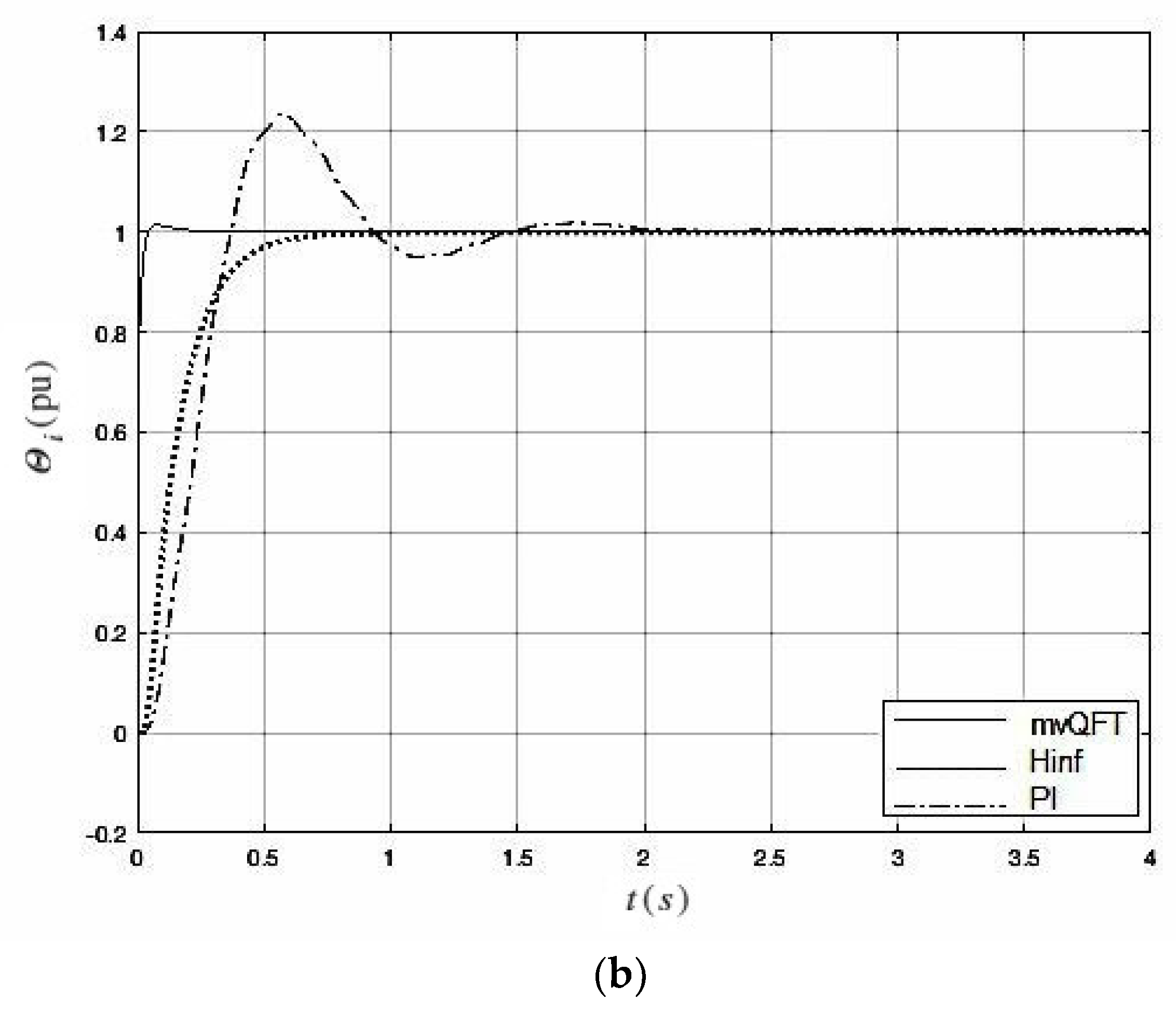
• Nominal Condition Test (N-test). Step responses of the nominal closed loop systems are obtained.
• Decupling Test (D-test). A step is applied on one reference input while the other remains zero, thus the impact of each reference input on the cross-coupling output is tested. The cross-coupling output response provides a measure of the column diagonal dominance of the closed loop system, i.e., the decoupling capabilities. Here, the value of such a response is referred to as “interaction level” (IL) and it is expected to be low. IL from θ_iref to σ_i is denoted as θ_i→σ_i, while σ_i→θ_i denotes that from σ_iref to θ_i. The nominal plant is used for this test. Although, in practice there are no standard limits for IL, in this work, an IL above 10% is considered to be undesirable.
• Parametric Uncertainty Test (U-test). Initially, each parameter takes a random value within its uncertainty region, changing randomly every 2s during the simulation time to allow the response to settle and confirm convergence. The methods used above to model the parametric uncertainties do not guarantee stability for the worst case; therefore, the parameters change randomly to test the system stability under the largest possible number of parameter value combinations (not under parameter variation, since the control techniques used here assume time-invariant uncertain parameters). During these tests, the perturbations inputs remain zero.
• Perturbation Test (P-test). This test is performed with the perturbation signals enabled, while the parameters remain constant on their operating values. Real signals of σ_i−1 and σ_i+1 were collected from the HSM and used for these tests. H_i and V_ri+1 were not available, hence sinusoidal signals are used to simulate them, taking each one a random frequency value between 0 Hz and 7 Hz independently. Their frequencies remain constant during the simulation time.
• Uncertainty and Perturbation Test (P+U-test). The conditions of U-test and P-test are combined.

For the sake of briefness, results for the N-test, D-test and P+U-test are shown only. The P+U-test was run a number of times due to its random nature and some of the results with the most critical responses were selected to be shown.

As mentioned, real signals of σ_i−1 and σ_i+1 were collected from the HSM, since the mill operates under small perturbation, some small perturbation tests were also run using the real σ_i-1 and σ_i+1 and simulated H_i and V_ri+1, obtaining similar results to those shown here. The perturbation signal frequency range for the P-tests and P+U-test was selected based on a Fourier analysis of several signals collected from the real mill, including σ_i−1 and σ_i+1.

Figure 9a,b shows the N-test responses.

Table 2. N-test step response characteristics.

Controller	σi			θi
	Mp	tp	ts	Mp	tp	ts
PI	43.4%	0.52 s	1.97 s	23.5%	0.56 s	1.364 s
H∞	null	null	1.012 s	null	null	0.55 s
mvQFT	42%	3.5 × 10−3 s	0.23 s	1.4%	0.075 s	0.32 s

shows the step response characteristics for each controller, the best characteristic by column is highlighted in bold characters. In Table 2, M_p is the maximum overshoot, t_p the time at which the maximum overshoot is presented, and t_s is the settling time using the 2% criterion. As can be seen, the best system in terms of M_p and t_p is that with the H_∞ controller, while in terms of t_s the mvQFT controller is the best. Note that the mvQFT controller presents a very short duration overshoot. It should be mentioned as well that the PI controllers were designed for the SISO loops, showing better responses when tested as such. In [18] the SISO QFT controller responses for the N-test are not presented, however they showed slower responses with larger M_p than H_∞ and mvQFT controllers. SISO QFT controllers also showed better responses when tested under SISO conditions.

The D-test responses are depicted in Figure 10a,b. Figure 10a shows θ_i→σ_i and Figure 10b shows σ_i→θ_i.

Table 3. Interaction levels.

Controller	σi→θi		θi→σi
	Transient	Steady State	Transient	Steady State
PI	−0.042	1.5 × 10−3	1.066	−0.5 × 10−3
H∞	0.8 × 10−3	null	0.24	null
mvQFT	−0.051	0.83 × 10−3	0.33	−0.03

shows the largest IL of each response during the transient and in steady state. The best IL by column is in bold characters. As can be seen, the H_∞ controller shows better decoupling capabilities than the mvQFT and PI, as expected since it is a full matrix MIMO TFM; however, the ILs with the mvQFT are satisfactory, less than 0.1 (10%). On the other hand, IL θ_i→σ_i with the PI controller is 1.066 pu (106.6%), which is unacceptable. The SISO QFT controllers in [18] showed higher interaction levels than H_∞ and mvQFT controllers, while in the case of θ_i→σ_i was even larger than that presented by PI controllers.

Figure 11 shows one of the most representative results of the P+U-Test. As can be seen, the responses with PI and H_∞ controllers show oscillations caused by the perturbation signals; the amplitudes are 130% and 87% larger with the PI controllers, for σ_i and θ_i respectively. The mvQFT have considerably better perturbation rejections. In Figure 11, the influence of the parameter changes can only be appreciated in σ_i response as some smaller and faster oscillations than those caused by the perturbations. This is consistent with the U-Test (not shown), the impact of the parameter changes is larger for σ_i than for θ_i. As can be seen in [18] the results for the P+U-Test are improved by the H_∞ and mvQFT controllers with respect to the response of the SISO QFT controllers.

In general, the controllers provide absolute stability robustness for the parameter combinations tested. However, the relative stability margins are significantly better for the mvQFT controllers, while the PI controllers showed the worst ones. In fact, in some tests run with PI controllers, the σ_i loop responses showed M_p values as high as 50%. For the parameter combinations tested here, the mvQFT controller showed better balance between M_p, t_p, t_s, IL and robustness than H_∞, PI, and SISO QFT [18] controllers; however, this is at the expenses of using greater power. The control signal power values for the three controllers are shown on

Table 4. Control input power.

Controller	τri	Vri
PI	4.5 × 10−12	3.6 × 10−9
H∞	4.5 × 10−12	5.4 × 10−9
mvQFT	3.7	6.8 × 10−9

. As can be seen, the power of τ_refi with mvQFT controller is significantly higher than the other control signals. This makes evident the need for the introduction of some control input power limitation criteria in the mvQFT controller designed in future.

A great disadvantage of the H_∞ control designed method used here is that a high order full matrix multivariable controller is produced, while the mvQFT is a diagonal TFM of 3rd order. As mentioned, different designs using different weighting function were tested, however there was not a significant impact on the H_∞ control order neither in the power requested by the mvQFT controller. Therefore, these problems should be particularly study in future.

6. Conclusions

Two multivariable robust controllers in the presence of parametric uncertainties for the 2 × 2 looper system were designed. These were a decentralized MIMO QFT and an H_∞ controllers, the former had not been applied before for the looper system. The parametric uncertainty was modeled in the frequency domain for both methodologies. The robustness conditions were verified in the frequency domain and time domain simulations were carried out. The performance of the design controllers was compared with each other and along with that of a PI controller and SISO QFT controllers designed earlier. In general, all controllers provided absolute stability robustness. The MIMO QFT controller showed the best balance among all performance indicators analyzed here: maximum overshoot, settling time, disturbance rejection, and interaction levels for different parameter sets; however, at the expense of using greater power on the looper torque control input. The results presented here showed the potential benefits brought by considering uncertainty and systems interactions during the controller designed stage, in this case by MIMO QFT and an H_∞ control techniques. There are some issues to addressed in future: (i) the design of H_∞ controllers of lower order than those designed here, (ii) to limit the power of the plant input for QFT technique, (iii) to study and overcome the problem of lack of tension measurement, and (iv) comparison with other techniques such as MPC and LMIs.

References

1. Roberts, W.L. Flat Processing of Steel; Marcel Dekker: New York, NY, USA, 1988; pp. 1–196. [Google Scholar]
2. Obregon, A.; Mendiola, P.; Evers, P.K.; Cavazos, A.; Leduc, L. Linear Multivariable Dynamic Model of a Hot Strip Finishing Mill. Proc. IMechE Part I J. Syst. Control Eng. 2010, 224, 1007–1021. [Google Scholar] [CrossRef]
3. Okada, M.; Murayama, K.; Urano, A.; Iwasaki, Y.; Kawano, A.; Shiomi, H. Optimal Control System for hot strip finishing mill. Control Eng. Pract. 1996, 6, 1029–1034. [Google Scholar] [CrossRef]
4. Cuzzola, F.A. A multivariable and multi-objective approach for control of hot-strip mills. J. Dyn. Syst. Meas. Contr. 2006, 128, 856–868. [Google Scholar] [CrossRef]
5. Zhan, M.; Yang, W.; Wang, S. Dual perturbation AGC design based on QFT/μ controller in hot strip rolling process. In Proceedings of the 29th Chinese Control Conference, Beijing, China, 29–31 July 2010; TCCT: Beijing, China, 2010; pp. 5682–5686. [Google Scholar]
6. Hyun-Hee, K.; Sung-Jin, K.; Min Cheol, L. The development of flying touch hot rolling control method based on SMCSPO. In Proceedings of the IEEE Conference on Advance Itelligent Mechatronics, Banf, AB, Canada, 12–15 July 2016; IEEE: New York, NY, USA, 2016; pp. 334–338. [Google Scholar]
7. Peng, W.; Yafeng, J.; Chen, S.; Zhang, D. Rolling characteristics analysis and dynamic roll force locking strategy for hot strip mill. J. Cent. South Univ. Sci. Tech. 2017, 48, 1492–1498. [Google Scholar]
8. Asano, K. Applications of model-driven control in steel processes. In Proceedings of the IFAC 18th World Congress, Milano, Italy, 28 August–2 September 2011; IFAC: Laxenburg, Austria, 2011; pp. 12096–12101. [Google Scholar]
9. Hearns, G.; Grimble, M.J. Multivariable control of a hot strip finishing mill. In Proceedings of the IEEE American Control Conference, Albuquerque, Mexico, 4–6 June 1997; IEEE: New York, NY, USA, 1997; pp. 3775–3779. [Google Scholar]
10. González Palacios, K.Y.; Cavazos González, A. Control robusto multivariable de espesor de cinta de acero y posición del formador de onda en un molino de laminación en caliente mediante H. In Proceedings of the IEEE Congreso Internacional sobre Innovación y Desarrollo Tecnológico, Cuernavaca, Mexico, 7–9 Septembre 2016; IEEE: Morelos, México, 2016; pp. 1–6. [Google Scholar]
11. Yu, C.; Wang, H.; Jing, Y. Tension control in hot strip process based on LMI approach. In Proceedings of the 23rd Chinese Control and Decision Conference, Mianyang, China, 23–25 May 2011; IEEE: New York, NY, USA, 2011; pp. 1424–1427. [Google Scholar]
12. Chen, J.X.; Yang, W.D.; Sun, Y.G. H control of looper tension control systems based on a discrete time model. J. Iron Steel Res. Int. 2013, 20, 28–31. [Google Scholar] [CrossRef]
13. Zhe, Y.; Ding, L.; Xiaoli, C.; Rui, W.; Fucai, Q.; Gang, Z. Decentralized robust decoupling control for looper tension and height system. In Proceedings of the 34th Chinese Control Conference, Hangzhou, China, 28–30 July 2015; IEEE: New York, NY, USA, 2015; pp. 1–6. [Google Scholar]
14. Hearns, G.; Grimble, J.M. Inferential control for rolling mills. IEEE Proc. Ctrl. Theory Appl. 2000, 147, 673–679. [Google Scholar] [CrossRef]
15. Hearns, G.; Grimble, J.M. Quantitative Feedback Theory for Rolling Mills. In Proceedings of the IEEE International Conference on Control Applications, Glasgow, UK, 18–20 September 2002; IEEE: New York, NY, USA; pp. 367–372. [Google Scholar]
16. Horowitz, I. Quantitative Feedback Theory. IEE Proc. Ctrl. Theory Appl. 1982, 129, 215–226. [Google Scholar] [CrossRef]
17. Sidi, M.J. Design of Robust Control Systems: From Classical to Modern Practical Approach; Krieger Publishing Company: Malabar, FL, USA, 2001; pp. 149–247. [Google Scholar]
18. Don Juan Ríos, O.A.; Rojas Lugo, E.A.; Cavazos González, A. Control robusto paramétrico QFT del sistema del formador de onda en un molino de laminación en caliente. Cienc. Ergo-Sum 2016, 23, 35–48. [Google Scholar]
19. Pliego Reyes, N.L.; Cavazos González, A. Control robusto del espesor de la cinta de acero en un molino de laminación en caliente mediante teoría de retroalimentación cuantitativa. In Proceedings of the Congreso Nacional de Control Automático, Monterrey, Mexico, 4–6 October 2017; AMCA: Mexico City, Mexico, 2017; pp. 213–219. [Google Scholar]
20. Choi, I.S.; Rossiter, J.A.; Fleming, P. An application of the model based predictive control in a hot strip mill. In Proceedings of the 11th IFAC Symposium on Automation in Mining, Mineral and Metal Processing, Nancy, France, 8–10 September 2004; IFAC: Laxenburg, Austria, 2004; pp. 131–136. [Google Scholar]
21. Choi, I.S.; Rossiter, J.A.; Fleming, P. Looper and tension control in hot rolling mills: A survey. J. Process Control 2007, 17, 509–521. [Google Scholar] [CrossRef]
22. Schuurmans, J.; Jones, T. Control of mass flow in a hot strip mill using model based predictive control. In Proceedings of the IEEE International Conference on Control Applications, Glasgow, UK, 18–20 September 2002; IEEE: New York, NY, USA, 2002; pp. 379–384. [Google Scholar]
23. Yin, F.C.; Sun, J.; Peng, W.; Wang, H.Y. Dynimic matrix predictive control for hydraulic looper system in hot strip mills. J. Cent. South Univ. 2017, 24, 1369–1378. [Google Scholar] [CrossRef]
24. Noh, I.; Won, S.; Jang, Y.J. Non-interactive looper and strip tension control for hot finishing mill using nonlinear disturbance observer. ISIJ Int. 2012, 6, 1092–1100. [Google Scholar] [CrossRef]
25. Zhong, Z.; Wang, J.; Zhang, J.; Li, J. Looper tension sliding mode control for hot strip finishing mills. J. Iron Steel Res. Int. 2012, 19, 23–30. [Google Scholar] [CrossRef]
26. Yaniv, O. Synthesis of uncertain MIMO feedback systems for gain and phase margin at different channel breaking points. Automatica 1992, 28, 1017–1020. [Google Scholar] [CrossRef]
27. ASM. Metals Handbook: Vol. 1: Properties and Selection: Irons, Steels and High-Performance Alloys; ASM International: Materials Park, OH, USA, 1990. [Google Scholar]
28. Skogestad, S.; Postlethwaite, I. Multivariable Feedback Control, Analysis and Design, 2nd ed.; John Wiley and Sons: West Sussex, UK, 2001; pp. 301–303, 309. [Google Scholar]
29. Hearns, G.; Grimble, J.M. Fault Tolerant Strip Tension Control. In Proceedings of the 1998 American Control Conference, Philadelphia, PA, USA, 24–26 June 1998; pp. 2992–2996. [Google Scholar]
Figure 1. Schematic of two contiguous stands in an FM.
Metals 09 00839 g001
Figure 2. (a) Block diagram of the multivariable linear model of two contiguous stands of an FM, and (b) One-block representation of the model.
Metals 09 00839 g002
Figure 3. (a) σ ¯ ( G ( s ) ) and σ _ ( G ( s ) ) , and (b) σ ¯ ( G ( s ) ) for all possible plants.
Metals 09 00839 g003
Figure 4. Two-degrees of freedom close loop system.
Metals 09 00839 g004
Figure 5. (a) General control configuration, (b) N-Δ structure, and (c) M-Δ structure.
Metals 09 00839 g005aMetals 09 00839 g005b
Figure 6. Boundaries and loop-shaping, (a) σi, and (b) θi.
Metals 09 00839 g006
Figure 7. (a) Stability robustness verification and (b) performance robustness verification.
Metals 09 00839 g007
Figure 8. (a) wO() (solid) and ιO(ω) (dashed-dotted), and (b) robustness stability condition (13) verification, σ ¯ ( T ) (solid), wO() (dashed) and ιO(ω) (dashed-dotted).
Metals 09 00839 g008aMetals 09 00839 g008b
Figure 9. N-Test results (a) σi, and (b) θi.
Metals 09 00839 g009aMetals 09 00839 g009b
Figure 10. D-Test results (a) σi and (b) θi.
Metals 09 00839 g010
Figure 11. P+U-Test results (a) σi and (b) θi.
Metals 09 00839 g011