Modeling and Design Optimization of A Shaft-Coupled Motor and Magnetic Gear

Abstract

This paper presents the modeling and design of an actuator consisting of an electrical motor and a magnetic gear. To minimize the overall actuator dimensions, both of the electromagnetic devices need to be optimally designed and matched. An issue in performing a simultaneous design as such arises from a high number of design variables that significantly increases the complexity of the optimization problem. A method to reduce the design variables is discussed in this paper, which is the application of response surface methodology (RSM) to represent the optimized torques of the electrical motor and magnetic gear as polynomial functions of their respective dimensions. Prior to the application of RSM, optimization problem statements are defined for the electrical motor and magnetic gear, for which the optimization objective and constraint functions are derived from analytical electromagnetic models of the considered electromagnetic devices.

1. Introduction

A common type of actuator used in robotic applications is a mechanically-geared electrical motor, which has a high torque within a relatively small volume. For specific applications such as soft robotics [1], however, it is not desirable to use mechanical gears due to the presence of static friction that degrades the force/torque control performance [2]—not to mention that mechanical gears are vulnerable in the event of torque overload.

A promising solution to address the previous shortcomings of mechanical gears is to replace them with magnetic gears [3], whose topology is depicted in Figure 1. In a magnetic gear, the torque between the rotating members (high-speed and low-speed rotors) are transmitted without mechanical contact, resulting in a major reduction of the static friction. Furthermore, the rotating members would slip when the load torque exceeds a certain level, giving an inherent overload protection.

There are two possibilities to integrate an electrical motor and a magnetic gear. The first one is a conventional shaft-coupled motor and gear as shown in Figure 2a. The second one is the so-called “pseudo” direct-drive motor [4] illustrated in Figure 2b, which integrates all the electromagnetic components belonging to an electrical motor and a magnetic gear. In this paper, the shaft-coupled motor and gear is the chosen one to be investigated as it has a smaller outer diameter, which is a desirable aspect in the considered application.

In robotic/mechatronic applications, the optimal selection of motor and (mechanical) gear transmission ratio is necessary for the overall system performance [5]. For this particular optimization problem, generally, a number of off-the-shelf candidate motors and gears are considered, from which a motor-gear pair is selected based on criteria such as dimension, mass and efficiency [5,6,7]. However, when stringent design requirements are considered, it would be preferable to design and optimize both motor and gear specifically for the intended application, as it would provide flexibility in selecting design parameters such as outer dimensions.

This paper presents a rapid method to simultaneously optimize an electrical motor and a magnetic gear for an application. For this purpose, high-accuracy analytical electromagnetic models of an electrical motor and a magnetic gear are developed based on the harmonic modeling method [8,9]. The models are used to derive the objective and constraint functions from optimization problem statements for the considered electromagnetic devices. Since the optimization of the motor and magnetic gear are treated simultaneously, there is a high number of design variables that are involved, resulting in a slow and computationally-intensive numerical optimization task. For that reason, a solution is proposed in this paper to reduce the number of design variables by representing the optimized torques of the motor and magnetic gear as polynomial functions of their respective dimensions, i.e., outer diameter and axial length. The polynomial functions are approximated by the application of response surface methodology (RSM) [10] on the optimization routines that are defined for the motor and magnetic gear. Based on these polynomial models and the reduced design variables, the simultaneous design optimization of the motor and magnetic gear can be performed rapidly.

2. Electromagnetic Modeling

2.1. Harmonic Modeling Method

The goal of applying the harmonic modeling method [9] is to obtain an accurate estimation of the static magnetic field behavior within different material regions of an electromagnetic device, from which quantities such as magnetic flux density and torque, can be calculated. Note that the following assumptions are adhered in the modeling of the rotary electromagnetic devices discussed in this paper:

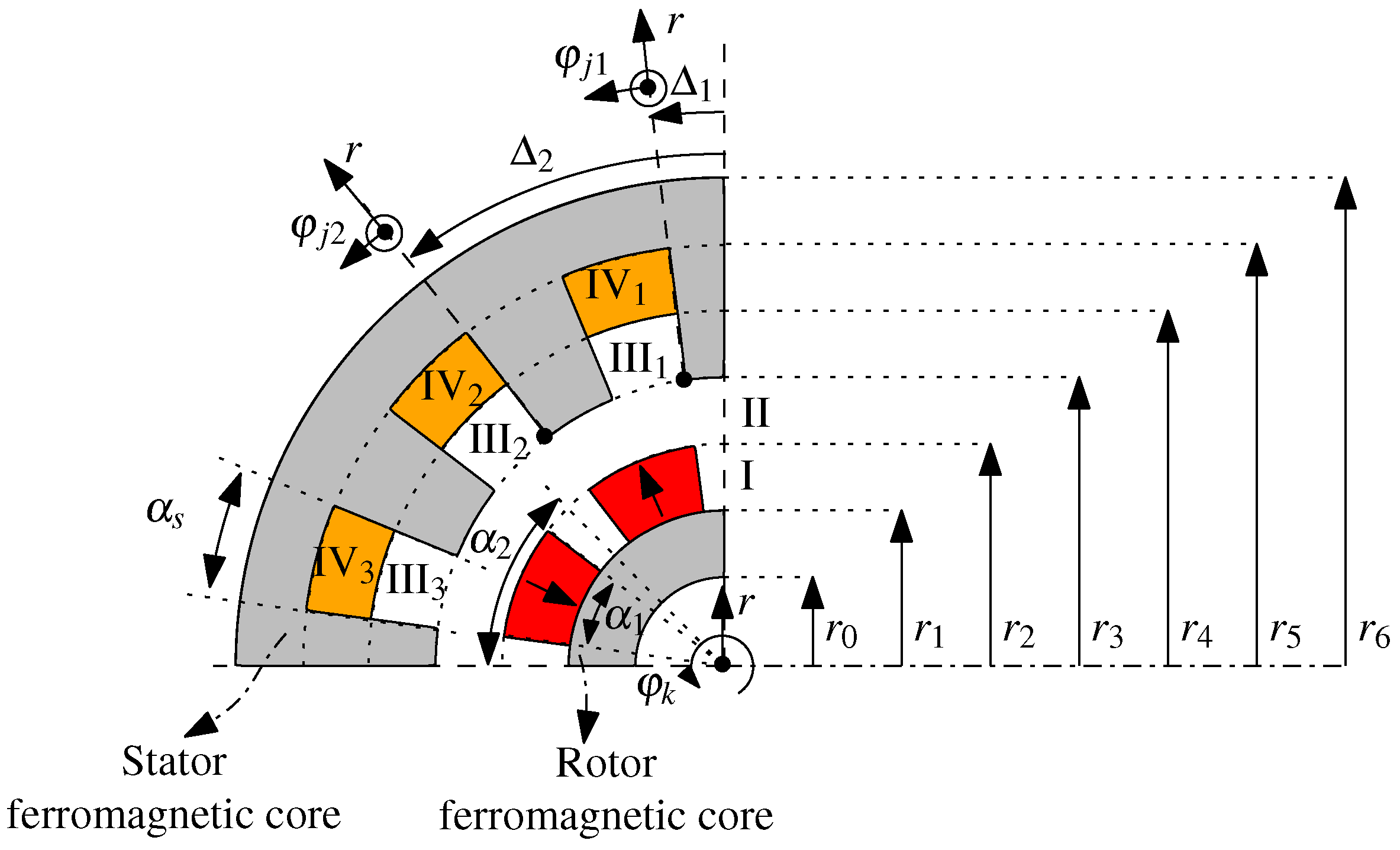
• The electromagnetic problem can be described in a 2D polar coordinate system ($r,\phi$)
• For a given region, the material has linear and homogenous magnetic properties in the r-direction.
• The ferromagnetic material is infinitely permeable. Consequently, no analytical expression of the magnetic flux density can be obtained within the ferromagnetic material.

As with the modeling of any electromagnetic devices, Maxwell’s equations govern the field behavior. From magnetostatic Maxwell equations, the following Poisson equation [8] is obtained

$${\nabla }^2\overrightarrow{A}=-{\mu }_0(\nabla \times \overrightarrow{M_0})-\mu \overrightarrow{J}$$

(1)

where $\overrightarrow{A}=A_z$ is the magnetic vector potential, ${\mu }_0$ is the vacuum magnetic permeability, μ is the material permeability, $\overrightarrow{M_0}=[M_r,M_{\phi }]$ is the residual magnetization vector and $\overrightarrow{J}=J_z$ is the current density vector. Considering a 2D polar coordinate system, the Poisson Equation (1) can be expressed as

$$\begin{array}{c}\hfill \frac{1}{r}\frac{\partial }{\partial r}r\frac{\partial A_z}{\partial r}+\frac{1}{r^2}\frac{{\partial }^2{A}_z}{\partial {\phi }^2}=-{\mu }_0\frac{1}{r}\left(\frac{\partial (r{M}_{\phi })}{\partial r}-\frac{\partial M_r}{\partial \phi }\right)-\mu J_z\end{array}$$

(2)

Within the investigated rotary electromagnetic devices, (circular) spatial periodicities are exhibited by the source terms in Equation (2), allowing them to be expressed by Fourier series

$$M_r=M_{r0}+\sum _{n=1}^N\left(M_{rs}sin(\frac{n\pi }{{\tau }_k}{\phi }_k)+M_{rc}cos(\frac{n\pi }{{\tau }_k}{\phi }_k)\right)$$

(3)

$$M_{\phi }=M_{\phi 0}+\sum _{n=1}^N\left(M_{\phi s}sin(\frac{n\pi }{{\tau }_k}{\phi }_k)+M_{\phi c}cos(\frac{n\pi }{{\tau }_k}{\phi }_k)\right)$$

(4)

$$J_z=J_{z0}+\sum _{n=1}^N\left(J_{zs}sin(\frac{n\pi }{{\tau }_k}{\phi }_k)+J_{zc}cos(\frac{n\pi }{{\tau }_k}{\phi }_k)\right)$$

(5)

where N is the number of harmonics to be modeled, $M_{r0}$, $M_{\phi 0}$ and $J_{z0}$ are DC components of the corresponding source terms ($M_r$, $M_{\phi }$, $J_z$); $M_{rs}$, $M_{rc}$, $M_{\phi s}$, $M_{\phi c}$, $J_{zs}$ and $J_{zc}$ are Fourier coefficients of the source terms, ${\tau }_k$ is half of the tangential width (ϕ-direction) of a material region k (within the electromagnetic device) and ${\phi }_k$ is the tangential position within the region k. Due to Equation (3), Equation (4) and Equation (5), the solution of the Poisson Equation (2), $A_z$, appears as a Fourier series. Given that $\overrightarrow{B}=\nabla \times \overrightarrow{A}$ (Gauss’ law of magnetic field), the magnetic flux density in the r and ϕ-directions for a given material region can also be expressed as Fourier series

$$B_r=\sum _{n=1}^N\left(B_{rs}sin(\frac{n\pi }{{\tau }_k}{\phi }_k)+B_{rc}cos(\frac{n\pi }{{\tau }_k}{\phi }_k)\right)$$

(6)

$$B_{\phi }=\sum _{n=1}^N\left(B_{\phi s}sin(\frac{n\pi }{{\tau }_k}{\phi }_k)+B_{\phi c}cos(\frac{n\pi }{{\tau }_k}{\phi }_k)\right)+B_{\phi 0}$$

(7)

where $B_{rs}$, $B_{rc}$, $B_{\phi s}$, $B_{\phi c}$ and $B_{\phi 0}$ are obtained from the solution of the Poisson Equation (2), given by:

$$B_{rs}=a_n{r}^{\frac{n\pi }{{\tau }_k}-1}+b_n{r}^{-\frac{n\pi }{{\tau }_k}-1}+G_{rs}$$

(8)

$$B_{rc}=-c_n{r}^{\frac{n\pi }{{\tau }_k}-1}-d_n{r}^{-\frac{n\pi }{{\tau }_k}-1}+G_{rc}$$

(9)

$$B_{\phi s}=c_n{r}^{\frac{n\pi }{{\tau }_k}-1}-d_n{r}^{-\frac{n\pi }{{\tau }_k}-1}+G_{\phi s}$$

(10)

$$B_{\phi c}=a_n{r}^{\frac{n\pi }{{\tau }_k}-1}-b_n{r}^{-\frac{n\pi }{{\tau }_k}-1}+G_{\phi c}$$

(11)

$$B_{\phi 0}=\frac{1}{2}\mu J_{z0}r+{\mu }_0{M}_{\phi 0}-\frac{A_0}{r}$$

(12)

where $a_n$, $b_n$, $c_n$, $d_n$ and $A_0$ in Equations (8)–(12) are obtained by considering the boundary conditions between the different material regions of the modeled electromagnetic device. The solutions for $G_{rs}$, $G_{rc}$, $G_{\phi s}$ and $G_{\phi c}$ are available in [8].

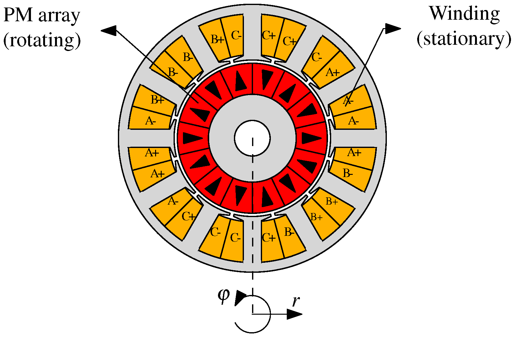
2.2. Harmonic Modeling of an Electrical Motor

The selected motor topology in this paper is the fractional-slot concentrated-windings PM motor [11] shown in Figure 3, which has favorable characteristics such as high torque density and low cogging [12]. For modeling purpose, the motor structure is represented by Figure 4. The structure is characterized by the material regions (I, II, etc.) described in

Table 1. Modeled regions in the motor, based on Figure 4.

Region	Description	Parameters
I	PM array	- Number of PM pole pairs, p
		- Pole-arc to pole-pitch ratio, ${\tau }_m=\frac{{\alpha }_1}{{\alpha }_2}$
		- Remanence, $B_r$
		- Relative permeability, ${\mu }_r$
II	Airgap	N/A
III${}_{1,\dots ,Q}$	Slot air	- Number of slots, Q
		- Slot opening, ${\alpha }_s$
IV${}_{1,\dots ,Q}$	Slot winding	- Number of slots, Q
		- Slot opening, ${\alpha }_s$
		- Current density, J

and parameters $r_0,...r_7$. Note that the slot winding regions IV${}_1$,...,IV${}_Q$ are simplified from its actual shape in Figure 3, as illustrated in Figure 5, in which $w_t$ denotes the tooth width. The equivalent current density of the winding $J_{eq}$ in Figure 5 is calculated as

$$J_{eq}=\frac{S_{actual}}{S_{simple}}\frac{J_1+J_2}{2}$$

(13)

where $S_{actual}$ and $S_{simple}$ are the cross-section areas of the actual and simplified slot winding, respectively, $w_t$ shown in Figure 5 is the tooth width, and $J_1$ and $J_2$ denote any adjacent current densities within a slot.

To obtain the expression for the magnetic flux density distribution throughout the investigated motor, Equation (6) and Equation (7) are defined for each of the regions (Table 1) and the corresponding unknown coefficients in Equations (8)–(12) are solved through a set of linear equations arising from the following boundary conditions:

• Neumann boundary condition
  This specifies the tangential magnetic field strength to be $H_{\phi }=0$ [8] at the boundary between two regions of which one has $\mu =\infty$, giving

  • Between region I and rotor ferromagnetic core ($r=r_1$)

    $$B_{\phi ,I}-{\mu }_0{M}_{\phi ,I}=0$$

    (14)
  • Between region IV${}_q$ and stator ferromagnetic core ($r=r_5$), for $q=1,...,Q$

    $$B_{\phi ,I{V}_q}=0$$

    (15)
• Continuous boundary condition
  By applying Maxwell equations at the interface between different regions [13], the boundary conditions $B_{r,k}=B_{r,k+1}$ and $H_{\phi ,k}=H_{\phi ,k+1}$ are obtained, where k and $k+1$ indicate adjacent regions having a finite permeability ($\mu \ne \infty$). Considering regions with the same tangential width, the following continuous boundary conditions are identified:

  • Between regions I and II ($r=r_2$)

    $$B_{r,I}=B_{r,II}$$

    (16)

    $$B_{\phi ,I}-{\mu }_0{M}_{\phi ,I}={\mu }_{r,in}{B}_{\phi ,II}$$

    (17)
  • Between regions III${}_q$ and IV${}_q$ and stator ferromagnetic core ($r=r_4$), for $q=1,...,Q$

    $$B_{r,II{I}_q}=B_{r,I{V}_q}$$

    (18)

    $$B_{\phi ,II{I}_q}=B_{\phi ,I{V}_q}$$

    (19)
• Combination of Neumann and continuous boundary conditions
  Each slot air region III${}_{1,\dots ,Q}$ has different tangential widths with respect to the radially adjacent airgap region II. This gives rise to a combination of both Neumann and continuous boundary conditions which hold at certain intervals between regions II and III${}_q$, for $q=1,\dots ,Q$:

  $$B_{r,II{I}_q}=B_{r,II},\mathrm{for}0\le {\phi }_{jq}\le {\alpha }_s$$

  (20)

  $$\begin{array}{cc}\hfill H_{\phi ,II}& =\sum _{q=1}^Q{H}_{{\phi }_{II{I}_q}},\mathrm{for}0\le {\phi }_{jq}\le {\alpha }_s,\hfill \\ & =0,\mathrm{elsewhere}\hfill \end{array}$$

  (21)
  The slots introduce tangential Neumann boundary conditions on region III${}_q$, resulting in $H_r=0$ at the tangential boundaries ${\phi }_{jq}=0$ and ${\phi }_{jq}={\alpha }_s$. Consequently, the cosine component of $B_r$ in in region III${}_q$ vanishes, resulting in $B_{rc}=0$ and $B_{\phi s}=0$. Therefore, the boundary condition Equation (20) can be expressed as

  $$\sum _{m=1}^M{B}_{rs,II{I}_q}sin\left(\frac{m\pi }{({\alpha }_s/2)}{\phi }_{jq}\right)=\sum _{n=1}^N{B}_{rs,II}sin\left(\frac{n\pi }{{\tau }_k}{\phi }_k\right)$$

  (22)

  where M denotes the number of modeled harmonics in region $II{I}_q$. To simplify Equation (22), a correlation technique is applied [8], resulting in

  $$B_{rs,II{I}_q}=\sum _{n=1}^N(B_{rs,II}{ϵ}_s+B_{rc,II}{ϵ}_c)$$

  (23)
  The boundary condition Equation (21) can be expressed as

  $$\begin{array}{c}\hfill \sum _{n=1}^N\left[\left(B_{\phi s_{II}}-{\mu }_0{M}_{\phi s_{II}}\right)sin\left(\frac{n\pi }{{\tau }_k}{\phi }_{II}\right)+\left(B_{\phi c_{II}}-{\mu }_0{M}_{\phi c_{II}}\right)cos\left(\frac{n\pi }{{\tau }_k}{\phi }_{II}\right)\right]=\\ \hfill \sum _{q=1}^Q\left[\sum _{m=1}^M\left[\left(B_{\phi c,II{I}_q}-{\mu }_0{M}_{\phi c,II{I}_q}\right)cos\left(\frac{m\pi }{({\alpha }_s/2)}{\phi }_{jq}\right)+B_{\phi 0,II{I}_q}\right]\right]\end{array}$$

  (24)

  which can be simplified through the correlation technique as follows:

  $$B_{\phi s_{II}}-{\mu }_0{M}_{\phi s_{II}}=\sum _{q=1}^Q\left[\sum _{m=1}^M\left[\left(B_{\phi c,II{I}_q}-{\mu }_0{M}_{\phi c,II{I}_q}\right){\kappa }_c+B_{\phi 0,II{I}_q}{\kappa }_0\right]\right]$$

  (25)

  $$B_{\phi c_{II}}-{\mu }_0{M}_{\phi c_{II}}=\sum _{q=1}^Q\left[\sum _{m=1}^M\left[\left(B_{\phi c,II{I}_q}-{\mu }_0{M}_{\phi c,II{I}_q}\right){\zeta }_c+B_{\phi 0,II{I}_q}{\zeta }_0\right]\right]$$

  (26)

  where ${ϵ}_s$, ${ϵ}_c$, ${\kappa }_c$, ${\kappa }_0$, ${\zeta }_c$ and ${\zeta }_0$ are the correlation terms (see [8] for the solutions).

2.2.1. Model Verification

The analytical model is verified by comparing the calculated spatial magnetic flux density distribution with that obtained from a 2D nonlinear FEM (Finite Element Method) model.

Table 2. Motor parameters for the model verification.

Parameter	Value
No. of PM pole pairs, p	7
No. of slots, Q	12
Inner shaft radius, $r_0$	2.7 mm
Inner ferromagnetic core outer radius, $r_1$	3.7 mm
Inner PM outer radius, $r_2$	5.7 mm
Inner airgap outer radius, $r_3$	6 mm
Slot air outer radius, $r_4$	6.5 mm
Slot winding outer radius, $r_5$	10.5 mm
Outer stator radius, $r_6$	12.5 mm
Axial length, L	18 mm
Slot opening, ${\alpha }_s$	5${}^{\circ }$
Tooth width, $w_t$	2 mm
PM pole-arc to pole-pitch ratio, ${\tau }_m$	1
PM remanence, $B_r$	1.39
PM relative permeability, ${\mu }_r$	1.05
Ferromagnetic core material (for FEM)	M330-35A
Current density, J	5 A/mm${}^2$

presents the motor parameters used for the model verification. As evident from Figure 6, there is an excellent agreement between the calculated airgap (region II) magnetic flux density from the analytical and FEM models. Furthermore, the simulation duration of the analytical model is significantly shorter than that of linear and nonlinear FEM models by factor 20 and 120, respectively, as apparent from

Table 3. Simulation duration of the analytical and FEM (Finite Element Method) models, as executed in a PC with Intel Core i5-2500 (3.3 GHz) processor, 16 GB RAM and 64-bit Windows 7 OS.

Duration
Analytical (Linear)	FEM (Linear)	FEM (Nonlinear)
0.05 s	1 s	6 s

.

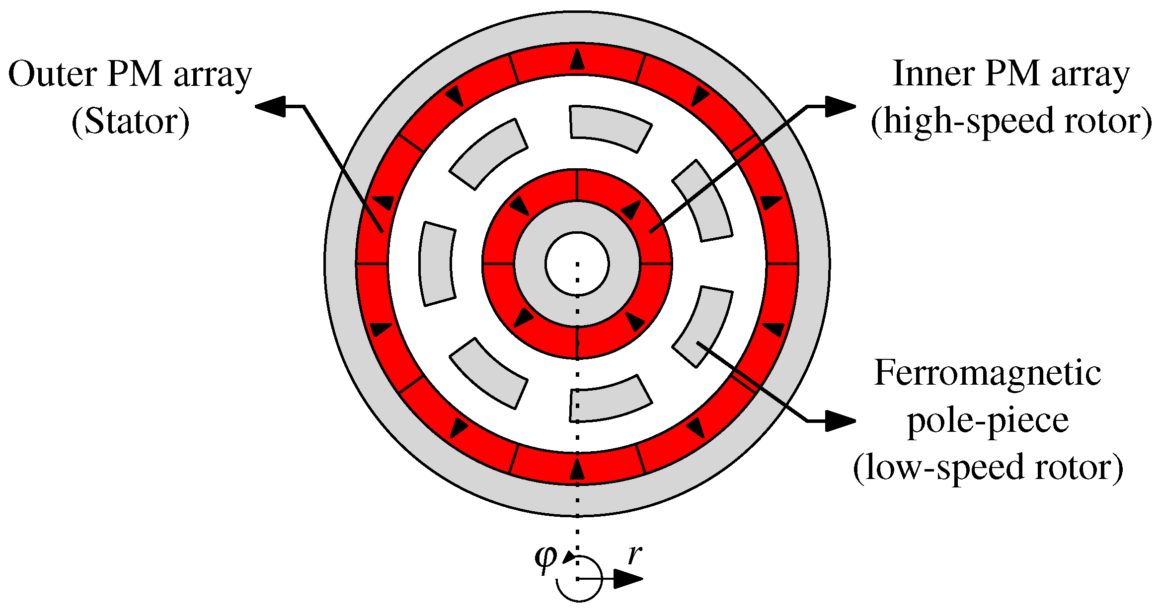
2.3. Harmonic Modeling of a Magnetic Gear

The considered magnetic gear topology in this paper is depicted in Figure 1, which for modeling purpose is represented by the structure in Figure 7. The modeled material regions (I, II, etc.) of the magnetic gear are described in

Table 4. Modeled regions in the magnetic gear.

Region	Description	Parameters
I	Inner PM array	- Number of inner PM pole pairs, $p_{in}$
		- Pole-arc to pole-pitch ratio, ${\tau }_{m,in}=\frac{{\alpha }_1}{{\alpha }_2}$
		- Remanence, $B_r$
		- Relative permeability, ${\mu }_r$
II	Inner airgap	N/A
III${}_{1,\dots ,Q}$	Air between pole-pieces	- Number of pole-pieces, Q
		- Tangential width, ${\alpha }_{pp}$
		- Pole-piece arc-to-pitch ratio, ${\tau }_Q=1-\frac{{\alpha }_{pp}}{2\pi /Q}$
IV	Outer airgap	N/A
V	Outer PM array	- Number of outer PM pole pairs, $p_{out}$
		- Pole-arc to pole-pitch ratio, ${\tau }_{m,out}=\frac{{\alpha }_3}{{\alpha }_4}$
		- Remanence, $B_r$
		- Relative permeability, ${\mu }_r$

.

As in the case of the electrical motor modeling, the magnetic flux density in the magnetic gear is obtained by considering the following boundary conditions:

• Neumann boundary condition at $r=r_1$ and $r=r_6$
• Continuous boundary condition at $r=r_2$ and $r=r_5$
• Combination of Neumann and continuous boundary conditions at $r=r_3$ (between regions II and III${}_{1,\dots ,Q}$) and $r=r_4$ (between regions IV and III${}_{1,\dots ,Q}$)
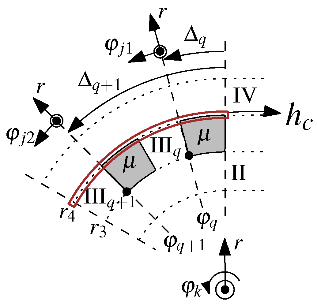
• Conservation of the magnetic flux around the pole pieces
  This boundary condition concerns Gauss’ law for magnetic field given by

  $${\oint }_S\overrightarrow{B}ds=0$$

  (27)
  By applying the the above to the pole-piece depicted in Figure 8, the following is obtained

  $$\begin{array}{cc}& {\int }_{{\phi }_q}^{{\phi }_{q+1}}{B}_{r,IV}{|}_{r=r_4}-{\int }_{{\phi }_q}^{{\phi }_{q+1}}{B}_{r,II}{|}_{r=r_3}+\hfill \\ & {\int }_{r_3}^{r_4}{B}_{\phi ,II{I}_{q+1}}{|}_{\phi ={\phi }_{q+1}}-{\int }_{r_3}^{r_4}{B}_{\phi ,II{I}_q}{|}_{\phi ={\phi }_q}=0\hfill \end{array}$$

  (28)

  for which $q=1,\dots ,Q-1$, with $Q-1$ being the number of independent equations. An extra equation is required to solve all the unknowns, obtained from the application of Ampere’s law at the pole-pieces radial boundary highlighted in Figure 8, as follows:

  $$\underset{h_c\to 0}{lim}{\oint }_C\overrightarrow{H}dl={\int }_S\overrightarrow{J}ds$$

  (29)

  for which J is zero, resulting in

  $$\sum _{q=1}^Q{\alpha }_{pp}{H}_{\phi ,II{I}_q}=2\pi H_{\phi ,IV}$$

  (30)

  where $h_c$ is the infinitesimal height of the boundary between region IV and III${}_q$. Since $B_{\phi 0,IV}=0$, the following is obtained:

  $$\sum _{q=1}^Q\frac{{\alpha }_{pp}}{{\mu }_0}{B}_{\phi 0,II{I}_q}=0$$

  (31)

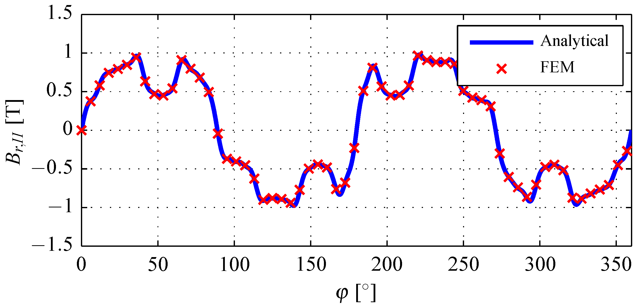
2.3.1. Model Verification

Table 5. Magnetic gear parameters for the model verification.

Parameter	Value
No. of inner PM pole pairs, $p_{in}$	2
No. of outer PM pole pairs, $p_{out}$	5
No. of pole-pieces, $Q=p_{in}+p_{out}$	7
Transmission ratio, $N_{mg}=\frac{Q}{P_{in}}$	3.5
Inner shaft radius, $r_0$	2.5 mm
Inner ferromagnetic core outer radius, $r_1$	4.5 mm
Inner PM outer radius, $r_2$	5.5 mm
Inner airgap outer radius, $r_3$	6 mm
Pole-piece outer radius, $r_4$	8.5 mm
Outer airgap outer radius, $r_5$	9 mm
Outer PM outer radius, $r_6$	10 mm
Stator outer radius, $r_7$	12.5 mm
Inner PM pole-arc to pole-pitch ratio, ${\tau }_{m,in}$	1
Outer PM pole-arc to pole-pitch ratio, ${\tau }_{m,out}$	0.9
Pole-piece arc to pitch ratio, ${\tau }_Q$	0.5
PM remanence, $B_r$	1.39
PM relative permeability, ${\mu }_r$	1.05
Ferromagnetic core material (for FEM)	Steel 1010

presents the magnetic gear parameters used for the model verification. As evident from Figure 9, there is an excellent agreement between the calculated airgap magnetic flux density distributions from the analytical and FEM models.

3. Definition of Optimization Problem Statements

To optimize the shaft-coupled motor and magnetic gear, optimization problem statements are defined separately for the two considered electromagnetic devices. A general optimization problem statement [14] is given as follows:

Minimize the objective function

$$f(\overrightarrow{X})$$

(32)

subject to inequality constraints

$$g_a(\overrightarrow{X})\le 0\mathrm{for}a=1,...,x$$

(33)

equality constraints

$$h_b(\overrightarrow{X})=0\mathrm{for}b=1,...,y$$

(34)

and bound constraints

$$X_c^l\le X_c\le X_c^u\mathrm{for}c=1,...,z$$

(35)

where $\overrightarrow{X}=[X_1{X}_2...X_o]$ is the design variable vector, $X_c^l$ and $X_c^u$ are the lower and upper bounds of a design variable, respectively. Based on the design requirements, the functions Equation (32), Equation (33) and Equation (34) are derived from the model of the investigated electromagnetic device. In this paper, the chosen optimization algorithm is the interior-point method [15] that can deal with nonlinear constraints and known for its speed and robustness [16].

3.1. Optimization Problem Statement for the Electrical Motor

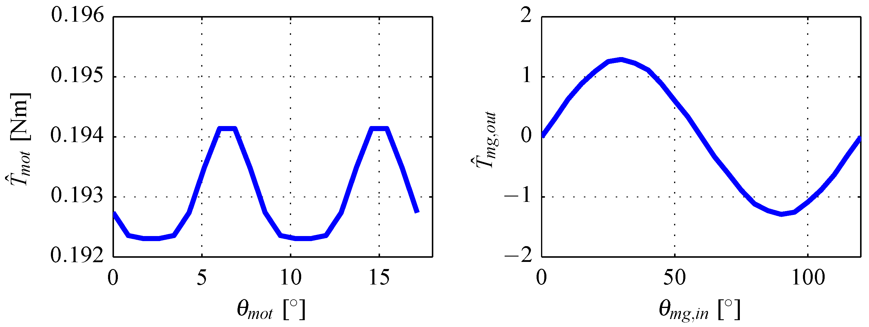
• Objective function
  The considered application requires that the motor and magnetic gear are compact and lightweight. An objective function that handles these requirements is the inverse of the mass torque density

  $$f_{mot}({\overrightarrow{X}}_{mot})=\frac{m_{mot}}{{\widehat{T}}_{mot}}$$

  (36)

  where $m_{mot}$ is the motor mass and ${\widehat{T}}_{mot}$ is the motor peak torque, defined as the highest level of torque that can be sustained for a period of time while the winding temperature rise does not exceed its limit. A thermal model is therefore developed, which is used to estimate the motor winding temperature and to derive the respective inequality constraint function (further described in the next part of this paper subsection).
  The motor torque $T_{mot}$ can be calculated using Maxwell stress tensor as follows:

  $$T_{mot}=\frac{L{r}_{in}^2}{{\mu }_0}{\int }_0^{2\pi }{B}_{r,II}{B}_{\phi ,II}d\phi$$

  (37)

  where L is the axial length, $r_{in}=\frac{r_2+r_3}{2}$ is the radius of the middle of airgap region II in Figure 4, $B_{r,II}$ and $B_{\phi ,II}$ are the radial and tangential magnetic flux densities in region II.
• Inequality constraint functions

  –

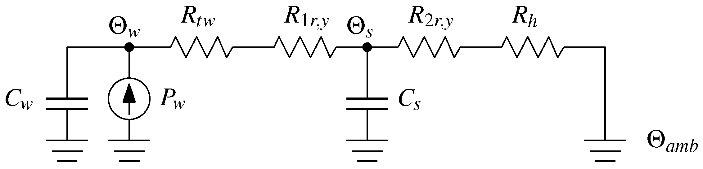
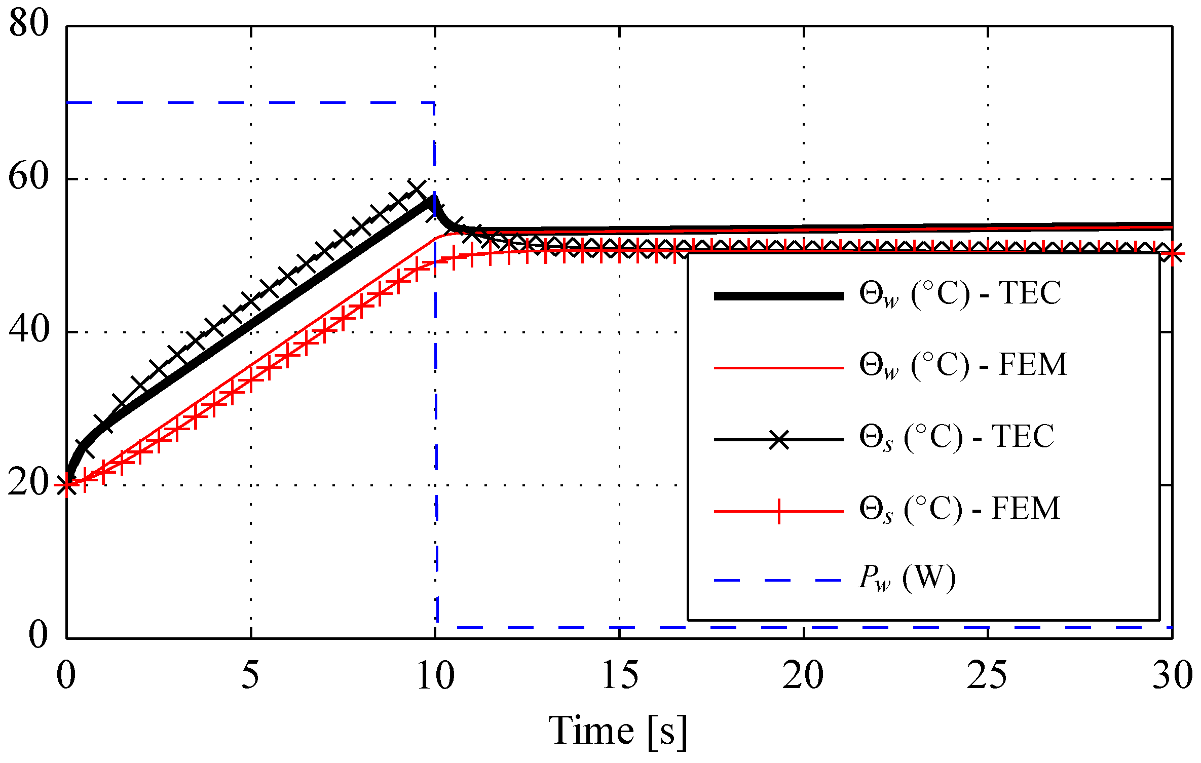
  Winding temperature

  Based on Equation (36), the following constraint on the peak torque is defined

  $$g_{1,mot}={\Theta }_{w,10s}\le 100{}^{\circ }C\mathrm{at}{\widehat{P}}_w$$

  (38)

  where ${\Theta }_{w,10s}$ is the winding temperature that can be sustained for 10 s (given that its initial temperature at time = 0 s is the same as the ambient temperature), while the peak winding copper loss ${\widehat{P}}_w$ is maintained. Note that core (iron) losses also contribute to the temperature increase, although this is neglected in the considered application since the motor maximum speed is 3000 rpm, which is relatively low for the investigated topology and this occurs only in a transient task. Ultimately, constraint function Equation (38) imposes a limit on the winding current density when the motor peak torque is applied. A simple transient thermal equivalent circuit (TEC) in Figure 10 is developed to estimate the temperatures in the winding (${\Theta }_w$) and stator (${\Theta }_s$) as functions of time, which are obtained by solving

  $$\left[\begin{array}{cc}\frac{1}{R_{tw}+R_{y,1}}& -\frac{1}{R_{tw}+R_{y,1}}\\ -\frac{1}{R_{tw}+R_{y,1}}& \frac{1}{R_{tw}+R_{y,1}}+\frac{1}{R_{y,2}+R_{conv}}\end{array}\right]\left[\begin{array}{c}{\Theta }_w\\ {\Theta }_s\end{array}\right]+\frac{d}{dt}\left[\begin{array}{cc}{C}_w& 0\\ 0& C_s\end{array}\right]\left[\begin{array}{c}{\Theta }_w\\ {\Theta }_s\end{array}\right]=\left[\begin{array}{c}{P}_w\\ \frac{{\Theta }_{amb}}{R_{y,2}+R_h}\end{array}\right]$$

  (39)

  where $R_{tw}$, $R_{y,1}$, $R_{y,2}$ are the radial conductive thermal resistances of the winding, stator yoke (inner and outer part), respectively, and $R_h$ is the convective thermal resistance (natural cooling is assumed). $C_w$ and $C_s$ are the thermal capacitances of the winding and stator, respectively. The calculation of thermal resistances and capacitances are based on the method described in [17]. The winding copper loss $P_w$ is calculated as

  $$P_w=\frac{Q{(J/\sqrt{2})}^2{\rho }_{cu}{l}_{coil}{S}_{coil}}{k_f}$$

  (40)

  where J is the current density, $l_{coil}$ is the single-turn length of a winding coil loop, $S_{coil}$ is the coil cross-section area and $k_f$ is the slot fill-factor. Figure 11 illustrated the temperatures of the motor winding and stator dynamically respond to the changes in copper loss, at ambient temperature of 20 ${}^{\circ }$C. A good agreement between TEC and FEM is apparent.

  –

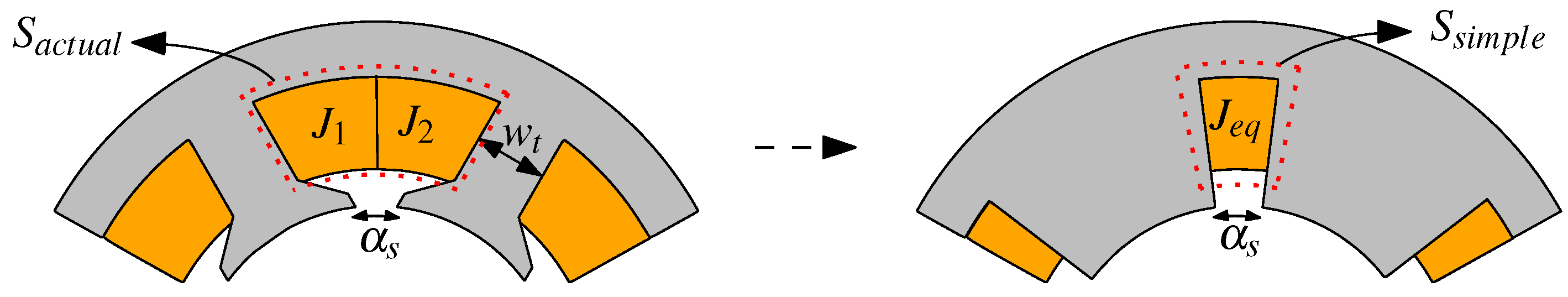
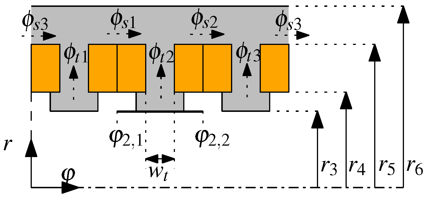
  Magnetic flux density in the ferromagnetic cores

  The used ferromagnetic core material has a typical saturation point at B = 1.5 T in its $B-H$ characteristic. Thus, to maintain a linear current-torque relation in the motor, the following constraint functions are defined

  $$g_{2,mot}({\overrightarrow{X}}_{mot})=B_t\le 1.5\mathrm{T}$$

  (41)

  $$g_{3,mot}({\overrightarrow{X}}_{mot})=B_s\le 1.5\mathrm{T}$$

  (42)

  where $B_t$ and $B_s$ are the magnetic flux density in the stator tooth and stator yoke, respectively, given by

  $$B_{ti}=\frac{{\varphi }_{ti}}{L{w}_t}$$

  (43)

  $$B_{sj}=\frac{{\varphi }_{si}}{L(r_6-r_5)}$$

  (44)

  where $w_t$ is the tooth width, ${\varphi }_{ti}$ and ${\varphi }_{sj}$ are the flux that goes through the i-th tooth and j-th yoke part (see Figure 12), respectively, estimated as

  $${\varphi }_{ti}=L{r}_3{\int }_{{\phi }_{i,1}}^{{\phi }_{i,2}}{B}_{II,r}d\phi$$

  (45)

  $${\varphi }_{sj}=-\frac{1}{Q}\sum _{j=1}^{Q-1}{\varphi }_{t\mathrm{mod}(j+i-1,Q)}$$

  (46)

  where mod($j+i-1,Q$) in (46) is a modulo operation, giving the remainder after division between $j+i-1$ and Q, while the integration limits ${\phi }_{i,1}$ and ${\phi }_{i,2}$ are depicted in Figure 12.

  –

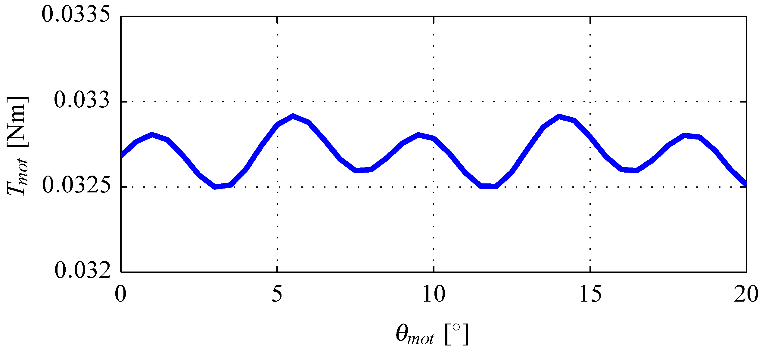
  Torque ripple

  A smooth torque characteristic is required in the considered application. For that reason, the ripple in the motor torque shown Figure 13 is constrained by the following function

  $$g_{4,mot}({\overrightarrow{X}}_{mot})=\frac{max({\widehat{T}}_{mot})-min({\widehat{T}}_{mot})}{{\widehat{T}}_{mot,avg}}\le 1\%$$

  (47)

  where ${\widehat{T}}_{mot}$ is the motor peak torque and ${\widehat{T}}_{mot,avg}$ is the average value of motor peak torque.

• Equality constraint functions
  A series of optimization tasks will be performed on the motor. For a given optimization task, fixed values of motor outer dimensions are assigned. Therefore, the following equality constraint on outer diameter $D_{mot}$ is introduced

  $$h_{1,mot}({\overrightarrow{X}}_{mot})=D_{mot}$$

  (48)

  Meanwhile, the motor axial length $L_{mot}$ is assigned as a design parameter.
• Design variables and bound constraints
  The design variable vector ${\overrightarrow{X}}_{mot}$ consists of motor geometric parameters (see Figure 4) and current density

  $${\overrightarrow{X}}_{mot}=[r_0,(r_1-r_0),(r_2-r_1),(r_3-r_2),(r_4-r_3),(r_5-r_4),(r_6-r_5),{\alpha }_s,{\tau }_m,w_t,J]$$

  (49)

  for which each variable adheres to the following lower and upper bound vectors (${\overrightarrow{X}}_{mot}^l$ and ${\overrightarrow{X}}_{mot}^u$, respectively),

  $${\overrightarrow{X}}_{mot}^l=\left[1\mathrm{mm},1\mathrm{mm},1\mathrm{mm},0.2\mathrm{mm},0.2\mathrm{mm},1\mathrm{mm},1\mathrm{mm},3^{\circ },0.5,1\mathrm{mm},\frac{J}{10}\right]$$

  (50)

  $${\overrightarrow{X}}_{mot}^u=\left[\frac{r_6}{2},\frac{r_6}{2},\frac{r_6}{2},\frac{r_6}{2},\frac{r_6}{2},\frac{r_6}{2},{15}^{\circ },\frac{r_6}{2},1,1\mathrm{mm},10J\right]$$

  (51)

3.2. Optimization Problem Statement for the Magnetic Gear

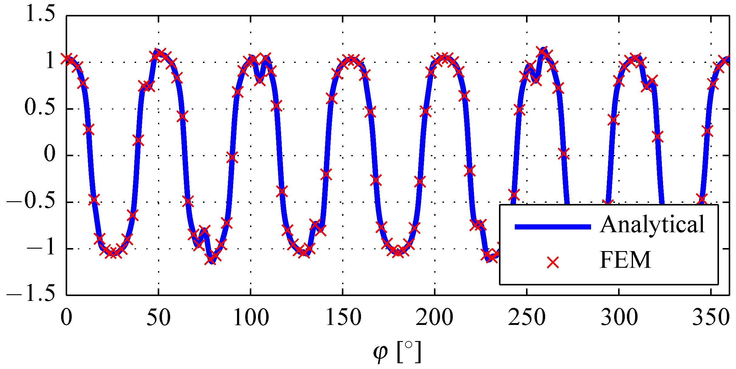
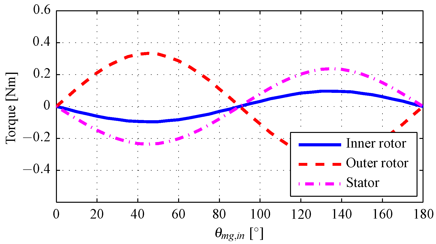
• Objective function
  Similar to the electrical motor optimization, the defined objective function of the magnetic gear is the inverse of mass torque density

  $$f_{mg}({\overrightarrow{X}}_{mg})=\frac{m_{mg}}{{\widehat{T}}_{mg,out}}$$

  (52)

  where $m_{mg}$ is the magnetic gear mass and ${\widehat{T}}_{mg,out}$ is the peak value of the outer rotor torque, which has a sinusoidal torque-position characteristic. This is shown in Figure 14 together with the torque characteristics of the inner rotor and stator. The outer rotor torque $T_{mg,out}$ is calculated as follows:

  $$\begin{array}{cc}\hfill T_{mg,out}& =T_{mg,stat}-T_{mg,in}\hfill \\ & =\frac{L{\left(\frac{r_4+r_5}{2}\right)}^2}{{\mu }_0}{\int }_0^{2\pi }{B}_{r,IV}{B}_{\phi ,IV}d\phi -\frac{L{\left(\frac{r_2+r_3}{2}\right)}^2}{{\mu }_0}{\int }_0^{2\pi }{B}_{r,II}{B}_{\phi ,II}d\phi \hfill \end{array}$$

  (53)

  where $T_{mg,stat}$ and $T_{mg,in}$ are the magnetic gear stator and inner rotor torque, respectively.
• Inequality constraint functions

  –

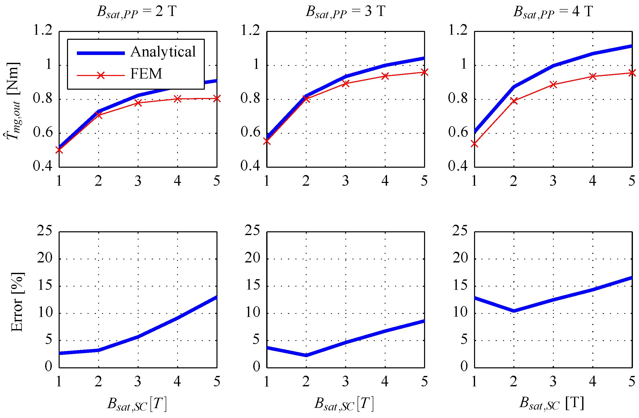
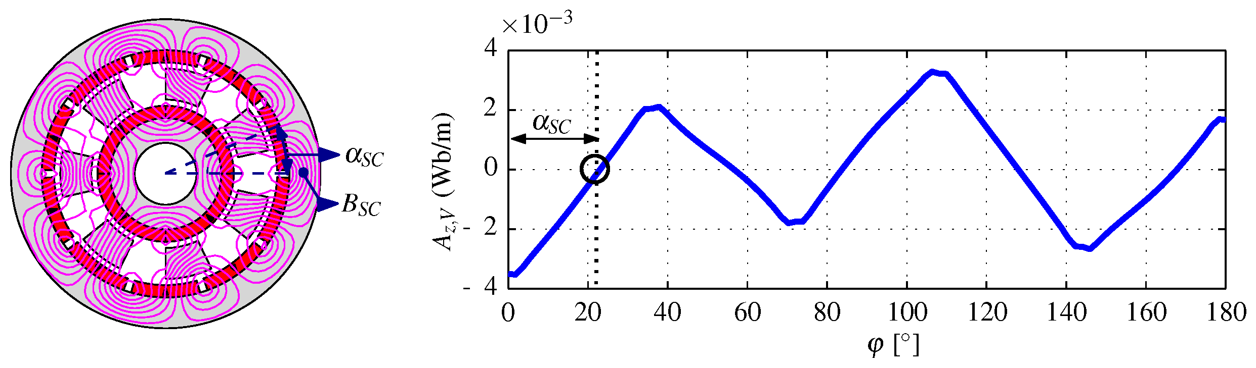
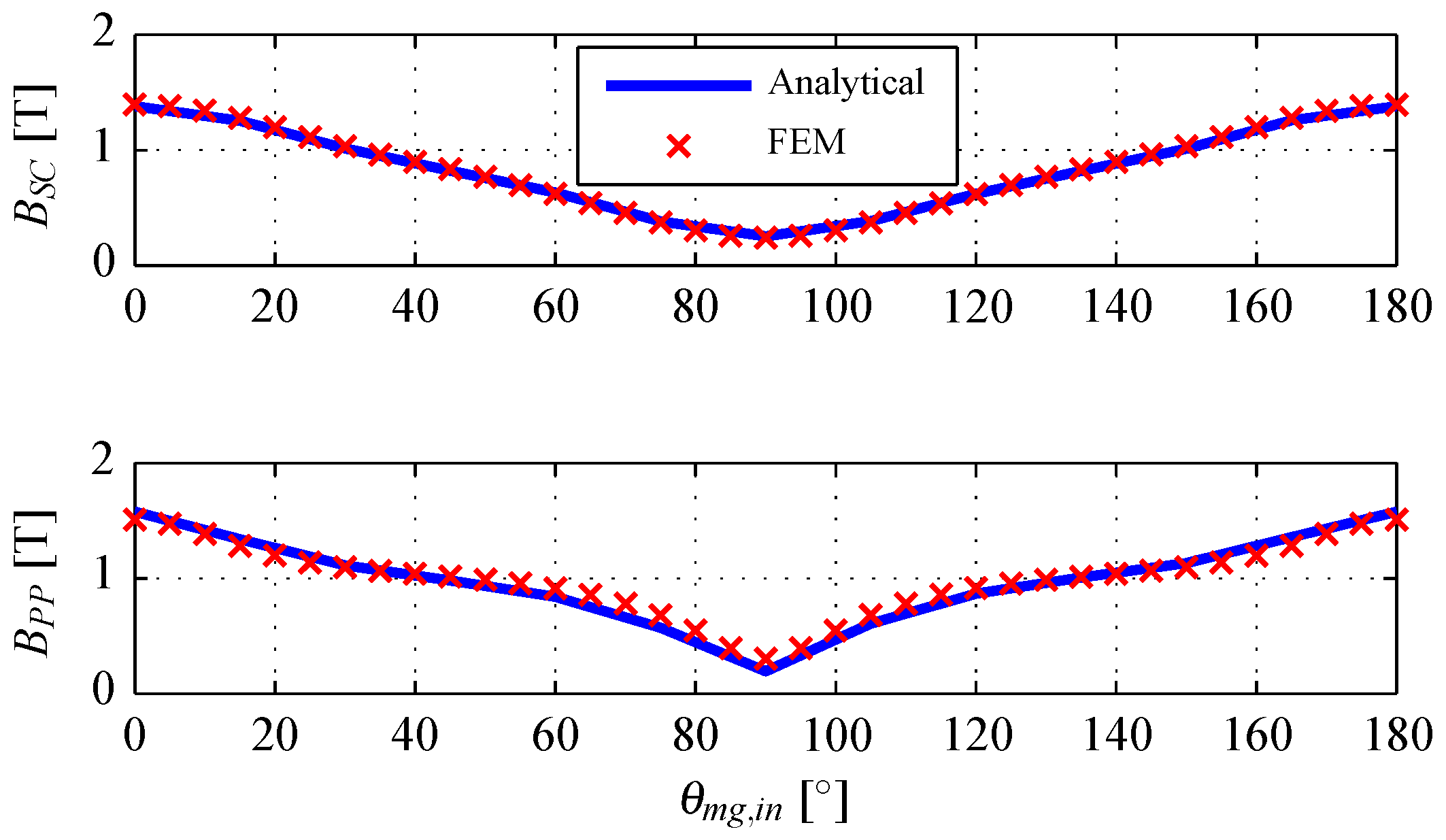
  Magnetic flux density in the ferromagnetic cores

  Constraints on the magnetic flux density in the pole-pieces and stator core of the magnetic gear are introduced to avoid saturation in the ferromagnetic cores, which leads to the inaccuracy of the analytical model with respect to the FEM model that accounts for nonlinear $B-H$ curve of the ferromagnetic steel 1010. The constraint values are selected such that the resulting torque is maximized while the analytical model accuracy is not significantly sacrificed. Figure 15 shows the variations of torque and discrepancy between analytical and FEM models for different values of the constraints $B_{sat,PP}$ and $B_{sat,SC}$, belonging to the pole-pieces and stator core, respectively. The constraints $B_{sat,PP}=3$ T and $B_{sat,PP}=3$ T as calculated by the analytical model are selected based on the previous consideration on torque and model accuracy; thus, the following constraint functions are defined:

  $$g_{1,mg}({\overrightarrow{X}}_{mg})=B_{SC}\le 3\mathrm{T}$$

  (54)

  $$g_{2,mg}({\overrightarrow{X}}_{mg})=B_{PP}\le 3\mathrm{T}$$

  (55)

  where $B_{SC}$ is the magnetic flux density in the stator core, estimated through

  $$B_{SC}=\frac{{\varphi }_{SC}}{L(r_7-r_6)}=\frac{L{r}_6{\int }_0^{{\alpha }_{SC}}{B}_{r,V}d\phi }{L(r_7-r_6)}$$

  (56)

  where ${\varphi }_{SC}$ is flux that enters the stator core over a range, from $\phi =0^{\circ }$ to $\phi ={\alpha }_{SC}$ as illustrated in Figure 16, for which the angle ${\alpha }_{SC}$ is determined from the zero crossing of the vector potential spatial distribution $A_{z,V}$ in region V. Meanwhile, $B_{PP}$ is the magnetic flux density in the pole-piece

  $$B_{PP}=\sqrt{B_{r,PP}^2+B_{\phi ,PP}^2}=\sqrt{{\left(\frac{1}{r_{PP}}\frac{\partial A_{z,PP}}{\partial \phi }\right)}^2+{\left(-\frac{\partial A_{z,PP}}{\partial r}\right)}^2}$$

  (57)

  where $A_{z,PP}$ is the vector potential distribution throughout regions III${}_1$,...,III${}_Q$ and the pole pieces, obtained through the the following linear interpolation

  $$A_{z,PP}=A_{z,II}\frac{r_4-r_{PP}}{r_4-r_3}+A_{z,IV}\frac{r_{PP}-r_3}{r_4-r_3}$$

  (58)

  where $A_{z,II}$ and $A_{z,IV}$ are the inner and outer airgap vector potential distributions, respectively, while $r_{PP}=\frac{r_3+r_4}{2}$ (see Figure 7 for $r_3$ and $r_4$). As can be seen from Figure 17, there is a good agreement between the analytical and FEM estimated values of $B_{SC}$ and $B_{PP}$.

• Equality constraint functions
  Following Equation (48), the following constraint on the magnetic gear outer diameter $D_{mg}$ is introduced

  $$h_{1,mg}({\overrightarrow{X}}_{mg})=D_{mg}$$

  (59)
  Additionally, the magnetic gear axial length $D_{mg}$ is fixed as a design parameter.
• Design variables and bound constraints
  The design variable vector ${\overrightarrow{X}}_{mg}$ consists of the magnetic gear geometric parameters (see Figure 7)

  $${\overrightarrow{X}}_{mg}=[r_0,(r_1-r_0),(r_2-r_1),(r_3-r_2),(r_4-r_3),(r_5-r_4),(r_6-r_5),(r_7-r_6),{\tau }_Q,{\tau }_{m,out}]$$

  (60)

  Each of the design variables has lower and upper bounds defined in the vectors ${\overrightarrow{X}}_{mg}^l$ and ${\overrightarrow{X}}_{mg}^u$, respectively, as follows:

  $${\overrightarrow{X}}_{mg}^l=[1\mathrm{mm},1\mathrm{mm},1\mathrm{mm},0.2\mathrm{mm},1\mathrm{mm},0.2\mathrm{mm},1\mathrm{mm},1\mathrm{mm},0.3,0.3]$$

  (61)

  $${\overrightarrow{X}}_{mg}^u=\left[\frac{r_7}{2},\frac{r_7}{2},\frac{r_7}{2},1\mathrm{mm},\frac{r_7}{2},1\mathrm{mm},\frac{r_7}{2},\frac{r_7}{2},0.7,1\right]$$

  (62)

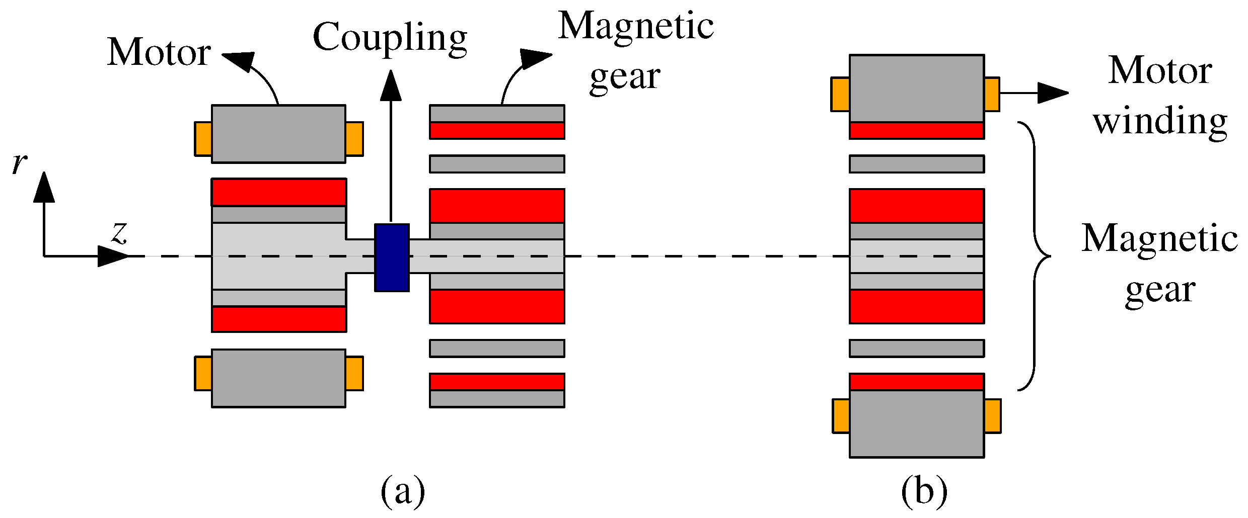
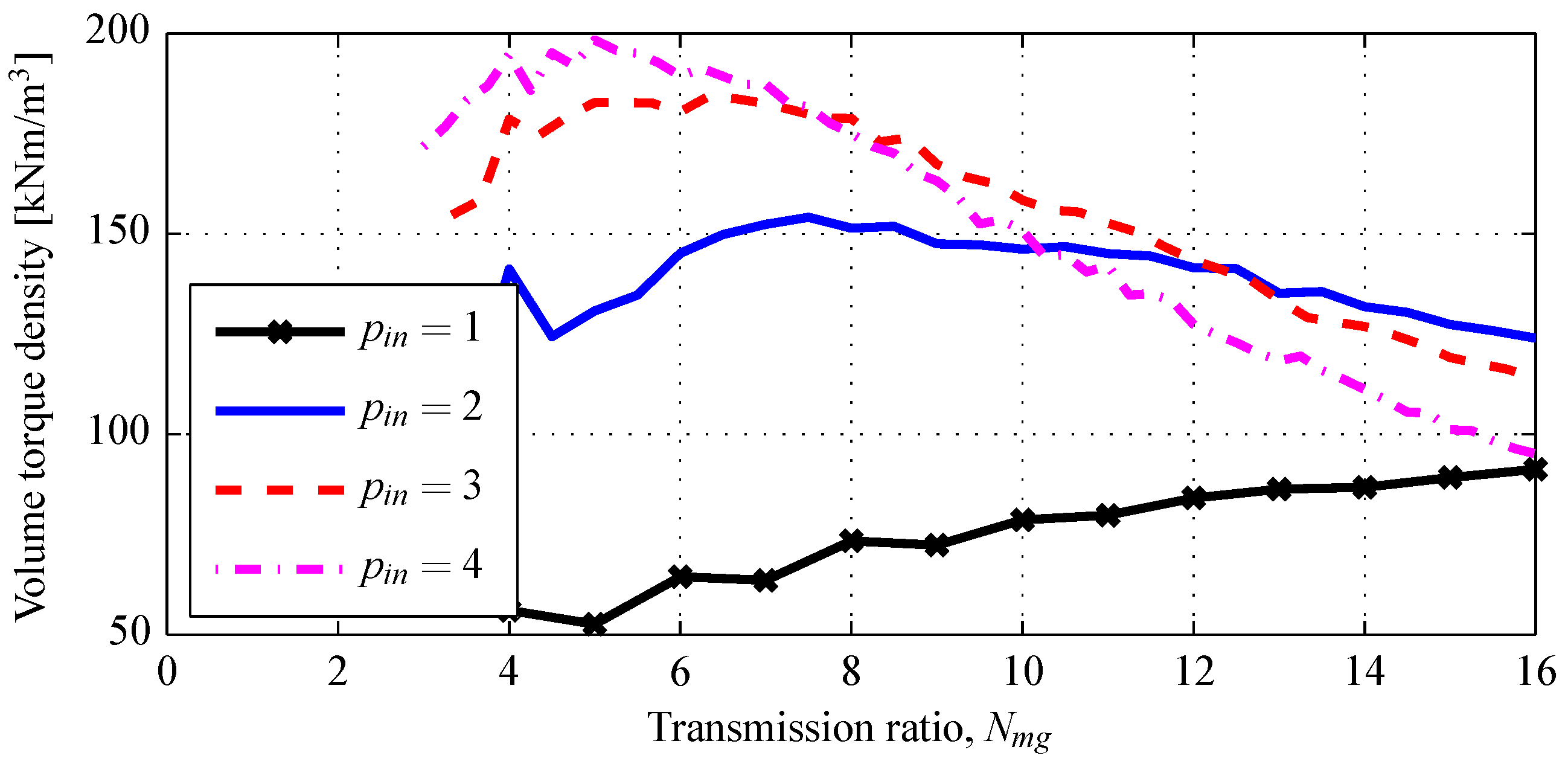
4. Optimization of the Shaft-Coupled Electrical Motor and Magnetic Gear

4.1. Modeling

The torque $T_{mmg}$ and speed ${\omega }_{mmg}$ of the shaft-coupled electrical motor and magnetic gear are expressed in terms of motor torque $T_{mot}$ Equation (37), speed ${\omega }_{mot}$ and magnetic gear transmission ratio $N_{mg}$ as follows:

$$T_{mmg}=N_{mg}{T}_{mot}$$

(63)

$${\omega }_{mmg}=\frac{{\omega }_{mot}}{N_{mg}}$$

(64)

where

$$N_{mg}=\frac{p_{in}+p_{out}}{p_{in}}$$

(65)

where $p_{in}$ and $p_{out}$ are the numbers of inner and outer PM pole pairs of the magnetic gear, respectively. Meanwhile the combined length of the integrated actuator, $L_{mmg}$, is given by

$$L_{mmg}=L_{mot}+L_{mg}+D_{mmg}$$

(66)

where $L_{mot}$ and $L_{mg}$ are the axial lengths of the motor and magnetic gear, respectively, and $D_{mmg}$ is the diameter of the integrated actuator, which is a factor to account for the extended length due to the shaft coupling and housing.

4.2. Design Requirements

The shaft-coupled electrical motor and magnetic gear will be used as an actuator in a robotic application that has to be compact and lightweight. These qualitative requirements are taken care by optimization objective functions Equations (36) and (52). An important design aspect to note related to the magnetic gear is the choices of inner PM pole pairs $p_{in}$ and transmission ratio $N_{mg}$, which significantly influence the optimized volume torque density as can be seen in Figure 18. As the numbers of PM pole pairs $p_{in}$ and $p_{out}$ (see Equation (65)) increase, the ferromagnetic cores become less prone to saturation and therefore they can be made thinner to improve the torque within a given magnetic gear volume. However, this improvement has its limitation since increasing the number of magnets implies smaller magnets that deliver less flux, and therefore the volume torque density is reduced again for higher $N_{mg}$ and $p_{in}$. Based on this and the characteristics in Figure 18, the values $p_{in}=3$ and $3.33\le N_{mg}\le 9.67$ are chosen for the design.

As for the quantitative requirements, the actuator has to deliver a peak torque of 1 Nm and has a maximum speed of 300 rpm. Note that from Equation (64), the required maximum speed can be achieved regardless of the magnetic gear transmission ratio, since the motor maximum speed is 3000 rpm (see Section 3.1). Additionally, there are following requirements related to dimensions

• The diameter of motor is equal to that of magnetic gear.
• The maximum axial length of the actuator is twice its diameter.

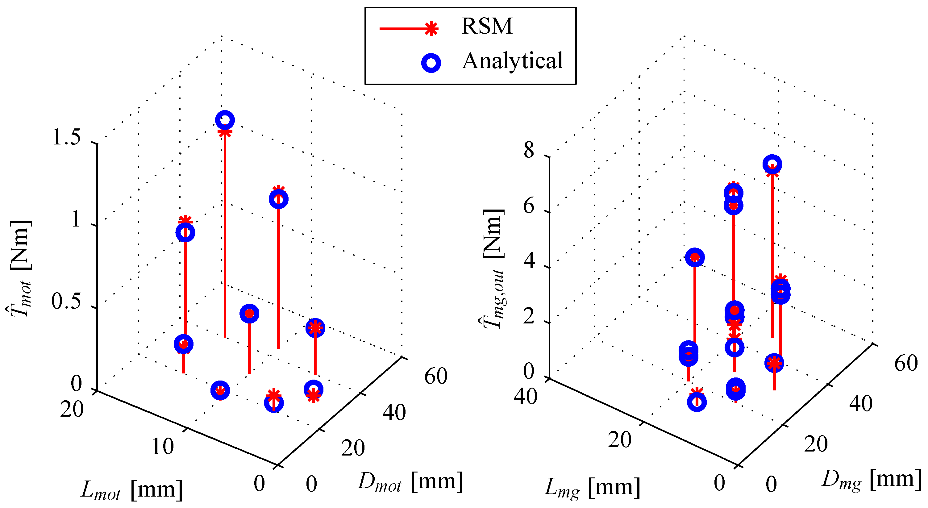
4.3. Response Surface Methodology

To reduce the computational burden associated with the simultaneous electrical motor and magnetic gear optimization, a major reduction of design variables, from 21 Equations ((49) and (60)) to five variables, is performed by expressing the electrical motor and magnetic gear peak torques as functions of their respective outer dimensions and transmission ratio, i.e., ${\widehat{T}}_{mot}(D_{mot},L_{mot})$ and ${\widehat{T}}_{mg,out}(D_{mg},L_{mg},N_{mg})$. The functions are approximated through the application of response surface methodology from a series of motor and magnetic gear optimization tasks.

Response surface methodology (RSM) is a technique to approximate a functional relationship between a response y and a number of input variables $x_1,x_2,...,x_k$ [10] of a given system. The approximated function is in the form of a first-order or the following second-order polynomial model:

$$y={\beta }_0+\sum _{i=1}^k{\beta }_i{x}_i+\sum _{i<j}\sum _j{\beta }_{ij}{x}_i{x}_j+\sum _{i=1}^k{\beta }_{ii}{x}_i^2+ϵ$$

(67)

where ${\beta }_0,{\beta }_i,{\beta }_{ij},{\beta }_{ii}$ are regressions coefficients and ϵ is a random error. Equation (67) can be expressed as

$$y=X\beta +ϵ$$

(68)

where X is a $n\times p$ matrix containing p variables from Equation (67) obtained from n experiments, β is a vector of regression coefficients and ϵ is a vector of random errors from n experiments. The estimated value of the regression coefficients vector, $\widehat{\beta }$, is obtained from the least-square method as follows [10]:

$$\widehat{\beta }={\left(X^{\prime }X\right)}^{-1}{X}^{\prime }y$$

(69)

In the context of this paper, an experiment refers to the set-up of the optimization design variable and parameter values that are chosen based on the Design of Experiment (DOE) method. Several DOE methods for first- and second-order polynomial models are described in [10]. The chosen DOE method in this paper is the popular one for approximating second-order models, i.e., Central Composite Design (CCD) [18,19].

To apply the CCD, a range of input variable values are initially selected. Based on pre-calculations, the following input variable range of values are expected to fulfil the design requirements

• 20 mm $\le D_{mot}\le$ 40 mm, 5 mm $\le L_{mot}\le$ 15 mm
• 20 mm $\le D_{mg}\le$ 40 mm, 10 mm $\le L_{mg}\le$ 20 mm, 3.33 $\le N_{mg}\le$ 9.67.

Next, CCD design matrices are defined for the motor and magnetic gear, as denoted by $D_{CCD,mot}$ and $D_{CCD,mg}$ in Equation (70) , respectively. Each matrix contains the normalized values of the previous input variable values, which are used as design parameters in the optimization problem statements in Section 3.1 and Section 3.2. Note that for a given optimization task, the electrical motor assumes the same values of p, Q, $B_r$, ${\mu }_r$ as in Table 2 while for the magnetic gear, the same values of $B_r$, ${\mu }_r$ in Table 5.

$${\mathrm{D}}_{CCD,mot}=\left[\begin{array}{cc}-1& -1\\ 1& -1\\ -1& 1\\ 1& 1\\ -\sqrt{2}& 0\\ \sqrt{2}& 0\\ 0& -\sqrt{2}\\ 0& \sqrt{2}\\ 0& 0\end{array}\right],{\mathrm{D}}_{CCD,mg}=\left[\begin{array}{ccc}-1& -1& -1\\ 1& -1& -1\\ -1& 1& -1\\ 1& 1& -1\\ -1& -1& 1\\ 1& -1& 1\\ -1& 1& 1\\ 1& 1& 1\\ -1.682& 0& 0\\ 1.682& 0& 0\\ 0& -1.682& 0\\ 0& 1.682& 0\\ 0& 0& -1.682\\ 0& 0& 1.682\\ 0& 0& 0\end{array}\right]$$

(70)

By applying the previously described RSM on a series of optimization tasks arising from the CCD design matrices Equation (70), the following polynomial models are obtained

$${\widehat{T}}_{mot}=\left[1D_{mot}{L}_{mot}(D_{mot}{L}_{mot})D_{mot}^2{L}_{mot}^2\right]{\widehat{\beta }}_{mot}^{\mathrm{T}}$$

(71)

$${\widehat{T}}_{mg}=\left[1D_{mg}{L}_{mg}{N}_{mg}(D_{mg}{L}_{mg})(D_{mg}{N}_{mg})(L_{mg}{N}_{mg})D_{mg}^2{L}_{mg}^2{N}_{mg}^2\right]{\widehat{\beta }}_{mg}^{\mathrm{T}}$$

(72)

where ${\widehat{T}}_{mot}$ and ${\widehat{T}}_{mg}$ are the optimized peak torques of the motor and magnetic gear, respectively, and the regression coefficients vectors ${\widehat{\beta }}_{mot}$ and ${\widehat{\beta }}_{mg}$ are given by

$${\widehat{\beta }}_{mot}=[0.8709-0.0513-0.09580.00450.00060.0006]$$

$${\widehat{\beta }}_{mg}=[2.236-0.2294-0.17180.28480.01030.00420.00080.00360.0003-0.0288].$$

The motor and magnetic gear peak torque values from the series of optimization tasks are shown in Figure 19. There is a good agreement between the torque values calculated from the RSM and analytical model. Based on this finding, the simple polynomial functions obtained from RSM, i.e., ${\widehat{T}}_{mot}(D_{mot},L_{mot})$ and ${\widehat{T}}_{mg,out}(D_{mg},L_{mg},N_{mg})$, are used for the optimization of the shaft-coupled motor and magnetic gear.

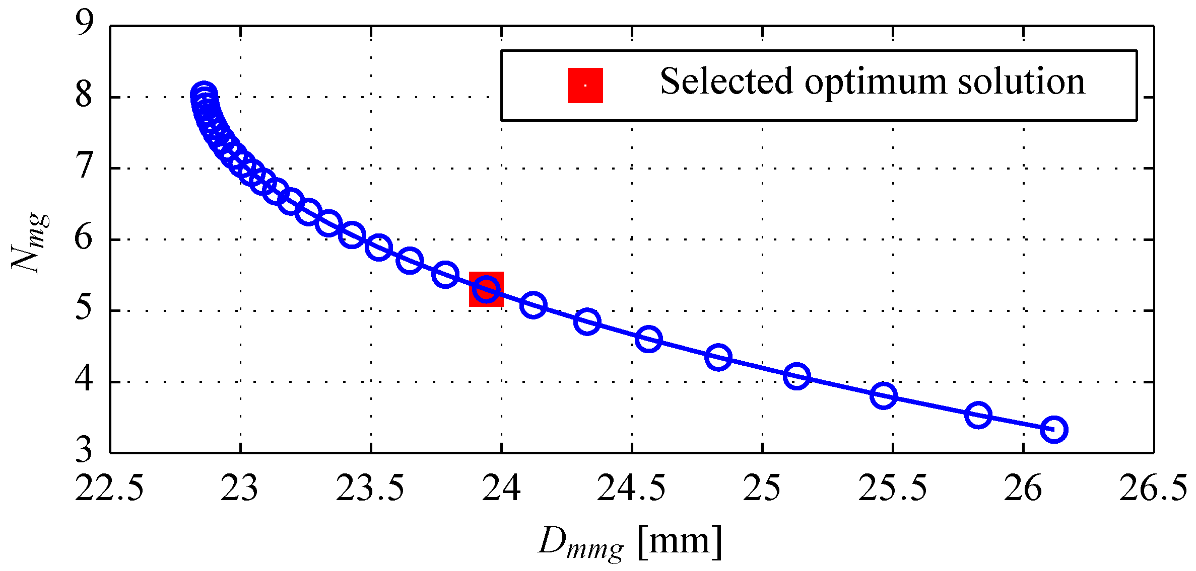
4.4. Definition of Optimization Problem Statement

Multiple objectives are considered in the optimization of the shaft-coupled motor and magnetic gear, namely for the minimization of outer diameter $D_{mmg}$ and transmission ratio $N_{mg}$. A single objective function can be formulated by the scalarization [20] of the two objective functions as follows:

$$f_{mmg}(\overrightarrow{X})={\mathrm{w}}_1{D}_{mmg}+{\mathrm{w}}_2{N}_{mg}$$

(73)

where w${}_1$ and w${}_2$ are linear weights (with $0\le$w${}_1\le 1$ and $0\le$w${}_2\le 1$) that will be varied in a series of optimization tasks to obtain a Pareto front. Meanwhile, the following constraints are defined based on the design requirements discussed in Section 4.2:

$$g_{1,mmg}(\overrightarrow{X})={\widehat{T}}_{mmg}\ge 1\mathrm{Nm}$$

(74)

$$g_{2,mmg}(\overrightarrow{X})=\frac{L_{mmg}}{D_{mmg}}\le 2$$

(75)

$$h_{1,mmg}(\overrightarrow{X})=D_{mot}=D_{mg}=D_{mmg}$$

(76)

Additionally, the following inequality constraint is imposed on the magnetic gear peak torque

$$g_{3,mmg}(\overrightarrow{X})={\widehat{T}}_{mg,out}\ge 120\%{\widehat{T}}_{mmg}$$

(77)

where the additional 20% in Equation (77) is a margin provided above the magnetic gear peak torque to prevent rotor slip. The design variable vector $X_{mmg}$ is given by

$$X_{mmg}=[D_{mot},L_{mot},D_{mg},L_{mg},N_{mg}]$$

(78)

for which the lower and upper bounds of the variables are based on the RSM input variable range of values in Section 4.3.

4.5. Results

Figure 20 depicts a Pareto front constructed from the objective function Equation (73), which is useful to evaluate design trade-offs between the magnetic gear transmission ratio $N_{mmg}$ and the outer diameter of the shaft-coupled motor and magnetic gear $D_{mmg}$. As the ratio between the weights in Equation (73), $\frac{{\mathrm{w}}_1}{{\mathrm{w}}_2}$ increases, the objective function minimization is emphasized on the diameter $D_{mmg}$, resulting in the decrease of motor and magnetic gear outer dimensions (see Equations (75) and (76)), while the magnetic gear transmission ratio $N_{mmg}$ increases. This illustrates how the magnetic gear ultimately contributes in reducing the motor size. On the other hand, it is also evident from Figure 20 that there is little improvement in motor size reduction for higher values of magnetic gear transmission ratios. This is caused the decrease of magnetic gear torque density as the transmission ratio increases after a certain value, as apparent from Figure 18. Additionally, from a practical point of view, a high magnetic gear transmission ratio implies more difficult manufacturing due to the increasing number of the required permanent magnets (see Equation (65)). Therefore, a specific optimum solution has to be chosen from Figure 20 to account for the trade-off between the transmission ratio and overall size of the shaft-coupled motor and magnetic gear.

The chosen optimum solution is marked in Figure 20, corresponding to the variable values $N_{mg}=5.3$, $D_{mot}=D_{mg}=24$ mm, $L_{mot}$ = 9.8 mm and $L_{mg}$ = 14.2 mm. The resulting magnetic gear transmission ratio has to match the transmission ratio Equation (65), with $p_i=3$. Furthermore, a specific value of the number of outer PM pole pairs $p_o$ has to be selected such that the resulting cogging torque is low [3,21]. Based on these considerations, $N_{mg}=5.33$ (which coincidentally is very close to the selected solution in Figure 20) is chosen as the transmission ratio value. A verification of the optimum solution is performed by separately re-optimizing the motor and magnetic gear using the analytical model as discussed in Section 3, based on the previous selected outer diameters, axial lengths and transmission ratio. The optimization results are shown in Figure 21, the average value of the motor peak torque is 0.19 Nm (resulting in ${\widehat{T}}_{mmg}=1.01$ Nm), while the magnetic gear outer rotor peak torque is 1.29 Nm, which fulfil the design requirements. By comparing the outer dimensions and volume of the shaft-coupled motor and magnetic gear, with those of an optimized electrical motor (having the same design requirements) in

Table 6. Comparison between outer dimensions and volume of the shaft-coupled motor and magnetic gear, and an electrical motor.

Parameter	Shaft-Coupled Motor and Magnetic Gear	Electrical Motor Only
Diameter	24 mm	30 mm
Axial length (incl. housing)	48 mm	45 mm
Volume	2.2$\times {10}^4$ mm${}^3$	3.2$\times {10}^4$ mm${}^3$

, there is an apparent benefit in terms of size reduction if the former actuator type is used.

5. Conclusions

An actuator based on a shaft-coupled electrical motor and magnetic gear is described in this paper. High-accuracy analytical electromagnetic models of the electrical motor and magnetic gear are developed and verified. Based on these models, design optimization objective and constraint functions are formulated in detail to account for electromagnetic and performance aspects such as magnetic saturation of the ferromagnetic cores, torque ripple/cogging and torque density.

For the simultaneous optimization of the electrical motor and magnetic gear, response surface methodology (RSM) is employed to reduce the number of design variables originating from the two electromagnetic devices, by representing their optimized torques as polynomial functions of their respective outer dimensions and transmission ratio (for the magnetic gear). A factor four of design variables reduction is achieved, and, as the polynomial functions are used to model the actuator, optimizations can be performed rapidly without sacrificing the accuracy of their results. From the constructed Pareto front, it is evident that the actuator size can be reduced by increasing the magnetic gear transmission ratio up to a certain level, after which the magnetic gear torque density limitation becomes more apparent and no further actuator size reduction can be achieved.

References

- Albu-Schaffer, A.; Eiberger, O.; Grebenstein, M.; Haddadin, S.; Ott, C.; Wimbock, T.; Wolf, S.; Hirzinger, G. Soft robotics. IEEE Robot. Autom. Mag. 2008, 15, 20–30. [Google Scholar] [CrossRef]
- Zanis, R.; Motoasca, E.; Lomonova, E. Trade-offs in the implementation of rigid and intrinsically compliant actuators in biorobotic applications. In Proceedings of the 2012 4th IEEE RAS EMBS International Conference on Biomedical Robotics and Biomechatronics (BioRob), Rome, Italy, 24–27 June 2012; pp. 100–105.
- Atallah, K.; Calverley, S.D.; Howe, D. Design, analysis and realisation of a high-performance magnetic gear. IEE Proc. Electr. Power Appl. 2004, 151, 135–143. [Google Scholar] [CrossRef]
- Atallah, K.; Rens, J.; Mezani, S.; Howe, D. A Novel Pseudo Direct-Drive Brushless Permanent Magnet Machine. IEEE Trans. Magn. 2008, 44, 4349–4352. [Google Scholar] [CrossRef]
- Roos, F.; Johansson, H.; Wikander, J. Optimal selection of motor and gearhead in mechatronic applications. Mechatronics 2006, 16, 63–72. [Google Scholar] [CrossRef]
- Van de Straete, H.; Degezelle, P.; De Schutter, J.; Belmans, R. Servo motor selection criterion for mechatronic applications. IEEE/ASME Trans. Mechatron. 1998, 3, 43–50. [Google Scholar] [CrossRef]
- Cusimano, G. Optimization of the choice of the system electric drive-device-transmission for mechatronic applications. Mech. Mach. Theory 2007, 42, 48–65. [Google Scholar] [CrossRef]
- Gysen, B.; Meessen, K.; Paulides, J.; Lomonova, E. General Formulation of the Electromagnetic Field Distribution in Machines and Devices Using Fourier Analysis. IEEE Trans. Magn. 2010, 46, 39–52. [Google Scholar] [CrossRef]
- Gysen, B.L.J. Generalized Harmonic Modeling Technique for 2D Electromagnetic Problesm: Applied to the Design of a Direct-Drive Active Suspension Systems. Ph.D. Thesis, Eindhoven University of Technology, Eindhoven, The Netherlands, 2011. [Google Scholar]
- Khuri, A.I.; Mukhopadhyay, S. Response surface methodology. Wiley Interdiscip. Rev. Comput. Stat. 2010, 2, 128–149. [Google Scholar] [CrossRef]
- EL-Refaie, A. Fractional-Slot Concentrated-Windings Synchronous Permanent Magnet Machines: Opportunities and Challenges. IEEE Trans. Ind. Electron. 2010, 57, 107–121. [Google Scholar] [CrossRef]
- Zhu, Z.Q. Fractional slot permanent magnet brushless machines and drives for electric and hybrid propulsion systems. COMPEL Int. J. Comput. Math. Electr. Electron. Eng. 2011, 30, 9–31. [Google Scholar]
- Furlani, E.P. Permanent Magnet and Electromechanical Devices; Academic Press: San Diego, CA, USA, 2001. [Google Scholar]
- Vanderplaats, G. Numerical Optimization Techniques for Engineering Design; Vanderplaats Research and Development, Inc.: Colorado Springs, CO, USA, 1999. [Google Scholar]
- Coleman, T.F.; Zhang, Y. Optimization Toolbox: User’s Guide (r2015b); MathWorks: Natick, MA, USA, 2015. [Google Scholar]
- Rokke, A. Gradient based optimization of Permanent Magnet generator design for a tidal turbine. In Proceedings of the 2014 International Conference on Electrical Machines (ICEM), Berlin, Germany, 2–5 September 2014; pp. 1199–1205.
- Mellor, P.; Roberts, D.; Turner, D. Lumped parameter thermal model for electrical machines of TEFC design. IEE Proc. B Electr. Power Appl. 1991, 138, 205–218. [Google Scholar] [CrossRef]
- Jolly, L.; Jabbar, M.; Qinghua, L. Design optimization of permanent magnet motors using response surface methodology and genetic algorithms. IEEE Trans. Magn. 2005, 41, 3928–3930. [Google Scholar] [CrossRef]
- Hasanien, H.; Abd-Rabou, A.; Sakr, S. Design Optimization of Transverse Flux Linear Motor for Weight Reduction and Performance Improvement Using Response Surface Methodology and Genetic Algorithms. IEEE Trans. Energy Convers. 2010, 25, 598–605. [Google Scholar] [CrossRef]
- Miettinen, K.; Makela, M.M. On scalarizing functions in multiobjective optimization. OR Spectr. 2002, 24, 193–213. [Google Scholar] [CrossRef]
- Zhu, Z.; Howe, D. Influence of design parameters on cogging torque in permanent magnet machines. IEEE Trans. Energy Convers. 2000, 15, 407–412. [Google Scholar] [CrossRef]