An Attempt to Use Non-Linear Regression Modelling Technique in Long-Term Seasonal Rainfall Forecasting for Australian Capital Territory

Abstract

The objective of this research is the assessment of the efficiency of a non-linear regression technique in predicting long-term seasonal rainfall. The non-linear models were developed using the lagged (past) values of the climate drivers, which have a significant correlation with rainfall. More specifically, the capabilities of SEIO (South-eastern Indian Ocean) and ENSO (El Nino Southern Oscillation) were assessed in reproducing the rainfall characteristics using the non-linear regression approach. The non-linear models developed were tested using the individual data sets, which were not used during the calibration of the models. The models were assessed using the commonly used statistical parameters, such as Pearson correlations (R), root mean square error (RMSE), mean absolute error (MAE) and index of agreement (d). Three rainfall stations located in the Australian Capital Territory (ACT) were selected as a case study. The analysis suggests that the predictors which has the highest correlation with the predictands do not necessarily produce the least errors in rainfall forecasting. The non-linear regression was able to predict seasonal rainfall with correlation coefficients varying from 0.71 to 0.91. The outcomes of the analysis will help the watershed management authorities to adopt efficient modelling technique by predicting long-term seasonal rainfall.

1. Introduction

Rainfall can be regarded as the most important climate element in the hydrological cycle that has considerable effects on the surrounding environment, including human lives. The spatial and temporal distribution of rainfall has significant impact on the water availability of earth surfaces, and hence on the agricultural activities. Since the agricultural activities and resulting crop production depends on the distribution of rainfall, prediction of monthly and seasonal rainfall is essentially important for the agricultural planning, flood mitigation strategies. However, accurate prediction of seasonal rainfall remains elusive to the scientists. Therefore, seasonal rainfall forecasting becomes plausible amongst the hydrologic researchers around the globe [1,2].

Seasonal forecasting can be classified into two broad categories: the statistical approach and the dynamic approach. In the statistical approach, the statistical relationships between the predictors and the predictands are investigated [3]. In the dynamic approach, seasonal meteorological estimates are used to build a hydrological model. However, there are methodological implications in using meteorological inputs in the current hydrological models [4]. The climate model produces the outputs based on coarse grid scales, which has the potential to capture forecasting uncertainties, and hence lead to bias. Furthermore, the data requirements of the dynamic models hinder the application of the modelling type. As a result, the statistical approach drew considerable attention to the practical users of the prediction models.

Long-term prediction of seasonal rainfall has the potential to help in the decision-making process for planning appropriate watershed management strategies [4]. Moreover, advanced prediction of rainfall can provide information to adopt the consequences of climate change [5]. As a result, the urge for the application of seasonal rainfall forecasting is increasing day by day. Therefore, seasonal forecasting is routinely performed by different research institutes, to have better understanding of climate change throughout the world. However, there exist limiting factors which act as the barriers for the wider application of the seasonal prediction models [6]. For example, the seasonal predictions are affected by the predictors, predictands, region and season [7]. Nevertheless, the chaotic dynamics of the atmosphere may lead to the erroneous prediction of seasonal rainfall [8]. The uncertainties in the model parameterization further hinder the prediction of seasonal rainfall.

Till today, precipitation is the most challenging climatic phenomena, which can be predicted with least accuracy [7]. On the other hand, most of the research studies on precipitation prediction have been conducted over a regional area of the world and in a particular season [9,10,11,12]. There exist only a few studies that concentrate on the precipitation analysis of the whole world [7,8,13]. Most of the studies conducted used number of various scores to evaluate predicted rainfall with the observed rainfall, such as, correlations, ranked probability score and Brier skill score. However, there is still doubt regarding the accuracy of the predictions of the seasonal models, which has immense implications in the decision-making process [14]. Nevertheless, there exists overconfidence and lack of reliability in the prediction of seasonal rainfall using the currently available models [15]. Therefore, it is necessary to assess the comprehensive performance of different models and their uncertainties in predicting seasonal rainfall.

It is well established that large-scale atmospheric circulation patterns significantly affect the annual precipitation around the globe including Australia. The atmospheric circulation configuration is dominated by the patterns of the sea surface temperature. Many researchers accept the capability of the El Nino Southern Oscillation (ENSO) in predicting time-series events. After analysing the role of ENSO on seasonal precipitation, Manzanas et al. [13] found that September to October is the most skillful season to predict rainfall around eastern Australia. Hossain et al. [9]; Hossain et al. [16] also identified the effects of ENSO and Indian Ocean Dipole (IOD) on West Australian rainfall. Therefore, the evaluation of the ENSO capability in time-series prediction is the fundamental requirement. Other climatic variables, such as sea surface temperature over the Atlantic and Indian Ocean have considerable impacts on the climate variability near the surrounding regions [17]. Recent studies also suggested that Indian Ocean Dipole (IOD) has the considerable effects on the climate variability in the continental regions including Australia [18,19]. Rasel et al. [20] revealed the effects of Southern Annular Mode (SAM) as a potential contributor of South Australian rainfall variability.

A number of studies have been examined to identify appropriate modelling technique for the prediction of seasonal rainfall. However, only a single climate driver is not capable of replicating the accurate precipitation characteristics. Multi-predictors models have the higher prediction skill than the single predictor models [21]. Nevertheless, there may exist dissimilar characteristics of seasonal rainfall patterns with the same rainfall totals [1]. On the other hand, there exist non-linear characteristics of the seasonal climate [8]. Therefore, a closer look at the appropriate mechanism of seasonal rainfall formation becomes essentially important.

This paper presents the efficiency of non-linear regression modelling technique in predicting long-term seasonal rainfall forecasting. The non-linear analysis was performed using the lagged (past) values of the climate indices as the potential predictors of long-term seasonal rainfall. Since there exist significant correlations between seasonal rainfall and two to three months average values of the climate indices, lagged values of the predictors were considered in this research. Furthermore, many researchers identified the ENSO and IOD as the most significant predictors of Australian seasonal rainfall. In this research, the efficiency of the climate indices in rainfall forecasting were assessed using the non-linear regression analysis technique. The non-linear analysis was performed considering South-eastern Indian Ocean (SEIO), Nino3.4 (sea surface temperature anomalies from 5° S to 5° N and 170° W to 120° W), southern oscillation index (SOI) and dipole model index (DMI) as the significant influential parameters of seasonal rainfall variation. The analysis was performed and applied to three rainfall stations in Australian Capital Territory (ACT). Seasonal rainfall forecasting can have practical implications to a wide range of users in diverse sectors, such as agriculture, energy, water supply and stormwater management [22]. The outcomes of the analysis may be the benchmark for future generations in predicting seasonal rainfall.

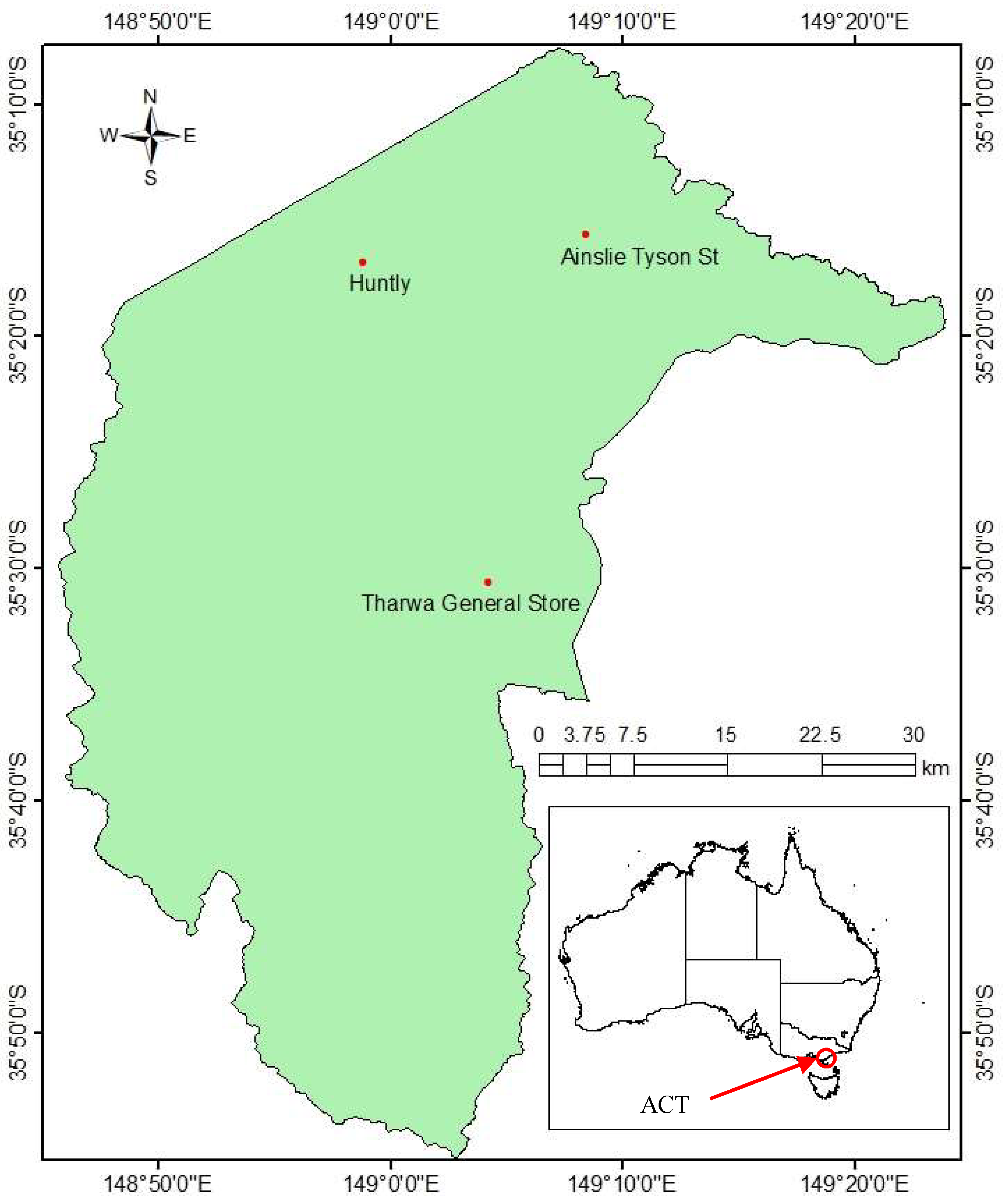
2. Study Area and Data Collection

The Australian Capital Territory (ACT) located in the south-east of the country is enclaved within the state of New South Wales (NSW). Unlike other Australian cities whose climates are moderated by the sea, the ACT experiences four distinct seasons. As a result, the inter-annual variation of precipitation in the ACT is higher. Annually, the ACT receives approximately 623 mm rainfall. The highest rainfall could be observed in spring and summer and the lowest in winter. This study concentrates on the application of non-linear regression modelling technique in the ACT for the prediction of long-term seasonal rainfall. The non-linear models were developed using the large-scale climate drivers. Therefore, the research requires both long-term rainfall data and climate indices data.

In Australia, the Bureau of Meteorology (BoM) collects and stores rainfall data from more than 2000 stations. For the achievement of the objectives of this paper, three rainfall stations located in the ACT were selected as a case study. Specific location of the rainfall stations is shown in Figure 1.

Long-term monthly rainfall data from 1971 to 2017 were downloaded from Australian Bureau of Meteorology (http://www.bom.gov.au/climate/data/?ref=ftr). The rainfall stations were selected based on the availability of long-term data which have fewer missing values. Monthly variation of the rainfall for the selected rainfall stations throughout the study period is shown in Figure 2. The long-term variation of the same rainfall could be seen in Figure 3 (blue curve). Seasonal rainfall was estimated from the collected monthly rainfall data. In this paper, the average of the spring (September-October-November) rainfall data were used to perform non-linear regression analysis. The data collected were used not only to construct the non-linear regression models but also to validate the prediction capability of the developed models.

To replicate the appropriate characteristics of seasonal rainfall, it is required to identify which month’s climate indices should be used in the analysis. Since the main focus of this paper is the efficiency of non-linear regression modelling technique in predicting long-term seasonal rainfall, the climate indices which have a significant correlation with rainfall were analysed and used for the construction of the non-linear models. Monthly values of the long-term climate indices data from 1971 to 2017 were collected from the climate explorer website (https://climexp.knmi.nl/start.cgi). Monthly values of the SEIO, Nino3.4, SOI and DMI were downloaded to achieve the objective of this research. In this paper, 90% of the data were used to construct the non-linear models and 10% of the data were used to assess the performance of the constructed models.

3. Methods

Traditional exploration of the relationship between two or more parameters are obtained by statistical regression analysis. In this study, non-linear regression analysis was performed to obtain steady relationship between long-term seasonal rainfall and large scale climate indices. In the non-linear regression technique, the arbitrary relationship between the predictands and predictors are obtained. One or more independent variables dictate the determination of non-linear relationship amongst the model parameters [23]. The general relationship of the non-linear regression can be explained according to Equation (1) [24]:

$$Y=b_1{X}_i+b_2{X}_j+b_3{X}_i^2+b_4{X}_j^2+\cdots ++b_n{X}_i{X}_j+e$$

(1)

where, Y is the dependent variable; b₁, b₂, ………b_n are coefficients of the independent variables; n is the number of observations; X is the independent variables and e is model error. The fitted model has the potential to predict the value of Y for the additional observed values of X.

There may exist different non-linear functions which is suitable to replicate the appropriate rainfall pattern. To find out the suitable predicting model for streamflow, researchers have performed a series of simple regression analysis [25]. To recommend a suitable seasonal rainfall predicting model, six different functions: linear, quadratic, cubic, exponential, power and logarithmic were assessed in this study. The function which has the higher Pearson correlation with the rainfall was considered as the potential model for rainfall prediction. The long-term seasonal rainfall data were used for the estimation of the correlations. The predictions may be penalized due to the lack of understanding of the physical processes. The interactions amongst the sub-processes of the variables may further hider the predictive capability [26]. Therefore, individual correlations amongst the climate indices were performed to assess the significant correlations. The climate indices which have significant correlation amongst themselves were not used to develop the non-linear regression models.

Since the forecast verification assesses the capability of re-producing the observed data, the process is considered as an essential process of any model development [27]. In this research, the assessment of the forecast quality of the developed non-linear regression models were performed using the commonly used statistical errors, Pearson correlations, root mean square error (RMSE), mean absolute error (MAE) and index of agreement (d). The regression model which has the highest correlation between the seasonal rainfall and combined indices during the validation period (2013–2017) was considered as the recommended predictor model.

4. Results and Discussion

From the available linear and non-linear functions, the Pearson correlations between the climate indices and the ACT spring rainfall was determined from the fitted data sets. The function which has the higher correlation was considered as the suitable model for rainfall prediction. The correlations of the regression analysis is shown in

Table 1. Pearson correlations of the regression analysis for Ainslie Tyson St station.

Index	Linear	Quadratic	Cubic	Exponential	Power	Logarithmic
DMIJun	0.083	0.097	0.154	0.082	0.182	0.187
NINO3.4Jun	0.420 *	0.428 *	0.436 *	0.411 *	0.153	0.157
NINO3.4Jul	0.462 *	0.462 *	0.495 *	0.456 *	0.056	0.061
NINO3.4Aug	0.503 *	0.503 *	0.524 *	0.499 *	0.332	0.338
SEIOJun	0.127	0.265	0.267	0.135	0.331	0.312
SEIOJul	0.208	0.280	0.323 *	0.218	0.305	0.309
SEIOAug	0.236	0.242	0.243	0.232	0.099	0.098
SOIJun	0.380 *	0.385 *	0.389 *	0.374 *	−0.055	0.071
SOIJul	0.407 *	0.407 *	0.470 *	0.405 *	0.451	0.242
SOIAug	0.502 *	0.517 *	0.527 *	0.488 *	0.002	0.002

,

Table 2. Pearson correlations of the regression analysis for Tharwa General Store station.

Index	Linear	Quadratic	Cubic	Exponential	Power	Logarithmic
DMIJun	0.193	0.198	0.226	0.190	0.183	0.192
NINO3.4Jun	0.457 *	0.480 *	0.507 *	0.440 *	0.232	0.240
NINO3.4Jul	0.518 *	0.519 *	0.573 *	0.508 *	0.089	0.099
NINO3.4Aug	0.542 *	0.542 *	0.589 *	0.533 *	0.298	0.303
SEIOJun	0.152	0.325 *	0.329 *	0.166	0.279	0.246
SEIOJul	0.195	0.253	0.301 *	0.204	0.226	0.230
SEIOAug	0.218	0.222	0.231	0.214	0.022	0.022
SOIJun	0.350 *	0.355 *	0.355 *	0.344 *	0.042	0.159
SOIJul	0.407 *	0.407 *	0.472 *	0.407 *	0.518 *	0.376
SOIAug	0.516 *	0.532 *	0.532 *	0.500 *	0.071	0.070

and

Table 3. Pearson correlations of the regression analysis for Huntly station.

Index	Linear	Quadratic	Cubic	Exponential	Power	Logarithmic
DMIJun	0.122	0.122	0.151	0.121	0.105	0.109
NINO3.4Jun	0.383 *	0.387 *	0.391 *	0.376 *	0.288	0.283
NINO3.4Jul	0.450 *	0.451 *	0.474 *	0.448 *	0.161	0.176
NINO3.4Aug	0.476 *	0.476 *	0.510 *	0.476 *	0.375	0.380
SEIOJun	0.136	0.260	0.280	0.136	0.268	0.246
SEIOJul	0.216	0.235	0.280	0.221	0.231	0.236
SEIOAug	0.248	0.258	0.274	0.241	0.076	0.076
SOIJun	0.267	0.274	0.274	0.262	−0.097	0.019
SOIJul	0.322 *	0.322 *	0.399 *	0.321 *	0.495 *	0.320
SOIAug	0.467 *	0.477 *	0.478 *	0.453 *	0.011	0.010

for Ainslie Tyson St, Tharwa General Store and Huntly rainfall stations respectively. The month shown in the subscript is the value of the corresponding climate index for the specified month. The star (*) in the table refers that the correlation is significant at the 0.05 level.

For Ainslie Tyson St rainfall station, the cubic function has the maximum correlations between spring rainfall and all the climate indices except SEIO_Jun. This climate index has the maximum correlation with power function as shown in Table 1. Similarly for Huntly rainfall station, the cubic function has the maximum correlations between spring rainfall and the climate indices except SOI_Jul. As evidenced in Table 2, power function has the maximum correlation with rainfall and this predictor. However for Tharwa General Store rainfall station, cubic function has the maximum correlations between spring rainfall and all the climate indices as can be seen in Table 3. Generally, the cubic function is the best predictor and the logarithmic function is the least predictor for seasonal rainfall forecasting. A similar outcome was obtained by Esha and Imteaz [25] in predicting streamflow.

To develop a generalised non-linear model for the prediction of seasonal rainfall, the functions which have the maximum correlation were further analysed. Seventeen combined non-linear models were developed for each of the rainfall stations. The arrangement was selected in such a way that there is no significant correlation amongst the input combinations. The correlation coefficients for each of the developed models were also estimated. The combined indices that have been used to construct the non-linear regression models and their correlations are shown in

Table 4. Pearson correlations of the developed models for the selected rainfall stations.

Indices Combination	Correlations
	Ainslie Tyson St	Tharwa General Store	Huntly
SEIOJun–Nino3.4Jun	0.533 *	0.620 *	0.485 *
SEIOJun–Nino3.4Jul	0.581 *	0.675 *	0.549 *
SEIOJun–Nino3.4Aug	0.589 *	0.661 *	0.556 *
SEIOJul–Nino3.4Jun	0.544 *	0.597 *	0.477 *
SEIOJul–Nino3.4Jul	0.587 *	0.646 *	0.537 *
SEIOJul–Nino3.4Aug	0.622 *	0.629 *	0.579 *
SEIOAug–Nino3.4Jun	0.463 *	0.537 *	0.444 *
SEIOAug–Nino3.4Jul	0.519 *	0.597 *	0.516 *
SEIOJun–SOIJun	0.472 *	0.489 *	0.400 *
SEIOJun–SOIJul	0.589 *	0.604 *	0.494 *
SEIOJun–SOIAug	0.602 *	0.616 *	0.530 *
SEIOJul–SOIJun	0.446 *	0.408 *	0.338 *
SEIOJul–SOIAug	0.619 *	0.625 *	0.547 *
SEIOAug–SOIAug	0.529 *	0.544 *	0.493 *
DMIJun–SOIJun	0.545 *	0.410 *	0.310 *
DMIJun–SOIJul	0.552 *	0.710 *	0.456 *
DMIJun–SOIAug	0.659 *	0.564 *	0.507 *

for all the selected three rainfall stations.

It is clear from Table 4 that only single model is not capable to predict seasonal rainfall with sufficient accuracy for all the rainfall stations. The table reveals that DMI-SOI based models are appropriate for predicting seasonal rainfall with maximum correlation 0.71. However, the appropriate combination is not in the same month for all the stations. For instance, DMI_Jun influence is dominant for all the three stations, whereas associated dominant indices are; SOI_Jul for Tharwa General Store station and SOI_Aug for Ainslie Tyson St station. For Huntley station, combined effect of SEIO_Jul and Nino3.4_Aug provided the highest correlation, with a Pearson correlation of 0.579. The outcomes support that the effects of climate indices vary spatially, and only single variable/index is not capable of predicting rainfall with sufficient accuracy. However, the combinations having higher correlations during the calibration were not considered as recommended models for rainfall prediction.

The combinations which produce maximum correlation during the validation period were considered to be the recommended models. For this case, SEIO_Jul–Nino3.4_Aug is the best model for the Ainslie Tyson St and Huntly stations; whereas SEIO_Jul–SOI_Aug is the highest correlation producers for Tharwa General Store station. Therefore, three models that have the highest correlation between the spring rainfall and the climate variables during the validation period have been proposed. Derirved models are outlined in Equations (2)–(4) for Ainslie Tyson St, Tharwa General Store and Huntly rainfall stations respectively.

$$\begin{array}{cc}\hfill {\left(\mathrm{Rainfall}\right)}_{\mathrm{Spring}}=& -74.0733\times {\mathrm{SEIO}}_{\mathrm{Jul}}^3+69.3359\times {\mathrm{SEIO}}_{\mathrm{Jul}}^2+11.5707\times {\mathrm{SEIO}}_{\mathrm{Jul}}\\ & +6.21085\times \mathrm{Nino}{3.4}_{\mathrm{Aug}}^3-1.57148\times \mathrm{Nino}{3.4}_{\mathrm{Aug}}^2-26.6653\hfill \\ & \times \mathrm{Nino}{3.4}_{\mathrm{Aug}}+54.6311\hfill \end{array}$$

(2)

$$\begin{array}{cc}\hfill {\left(\mathrm{Rainfall}\right)}_{\mathrm{Spring}}=& -91.0857\times {\mathrm{SEIO}}_{\mathrm{Jul}}^3+71.6046\times {\mathrm{SEIO}}_{\mathrm{Jul}}^2+12.3435\times {\mathrm{SEIO}}_{\mathrm{Jul}}\\ & -1.5962\times {\mathrm{SOI}}_{\mathrm{Aug}}^3-3.07473\times {\mathrm{SOI}}_{\mathrm{Aug}}^2+20.7424\times {\mathrm{SOI}}_{\mathrm{Aug}}\\ & +57.8264\hfill \end{array}$$

(3)

$$\begin{array}{cc}\hfill {\left(\mathrm{Rainfall}\right)}_{\mathrm{Spring}}=& -91.5749\times {\mathrm{SEIO}}_{\mathrm{Jul}}^3+69.4111\times {\mathrm{SEIO}}_{\mathrm{Jul}}^2+20.8865\times {\mathrm{SEIO}}_{\mathrm{Jul}}\hfill \\ & +8.33879\times \mathrm{Nino}{3.4}_{\mathrm{Aug}}^3-1.96053\times \mathrm{Nino}{3.4}_{\mathrm{Aug}}^2+33.6301\hfill \\ & \times \mathrm{Nino}{3.4}_{\mathrm{Aug}}+59.2245\hfill \end{array}$$

(4)

Since the cubic function has the potential to produce the higher correlation between seasonal rainfall and the considered climate indices, the equations have been developed for the cubic function. The combined capability of other functions will be assessed in future.

The plotted comparison of the analysis during the calibration period is shown in Figure 3. According to Figure 3, the non-linear regression models are not capable to replicate the actual seasonal rainfall with considerable accuracy. The statement is especially true for the extreme rainfall. When the rainfall is extremely high or extremely low, the approach is unable to capture the rainfall characteristics as evidence in Figure 3. More sophisticated analysis needs to be performed to replicate the extreme seasonal rainfalls. However, before concluding general remark, analysis on other area should be performed.

The plotted results of the prediction comparison during the validation period is shown in Figure 4. According to Figure 4, non-linear regression models should be used carefully to predict the seasonal rainfall with reasonable accuracy. To some extent, the approach is capable to predict the rainfall for some stations. For example, the approach is over predicting for Huntley rainfall station as evidence in Figure 4c. Therefore, other sophisticated modelling approaches should be explored for more accurate predictions of seasonal rainfall.

To evaluate the performance of the non-linear models developed, various statistical parameters were calculated. The outputs of the comparison are shown in

Table 5. Estimated statistical parameters during validation period.

Parameters	Ainslie Tyson St	Tharwa General Store	Huntly
R	0.91	0.71	0.86
RMSE	15.62	10.68	23.08
MAE	14.2	9.0	20.9
d	0.71	0.82	0.56

. According to the table, the model with correlation more than 0.91 has higher RMSE and MAE than the model with correlation 0.71. In addition, models with correlation 0.86 is having more errors than the other two models. Similar outcomes were also observed for the index of agreement. Therefore, models which have higher correlation do not necessarily produce a lower error rate. The index of agreement close to one is considered to be the best predicting model. Therefore, the models could be used to predict seasonal rainfall with reasonable accuracy. However, the analysis should be performed with more rainfall stations in the same area and other states.

5. Conclusions and Recommendations

Over the last two decades, prediction of seasonal time-series events were given considerable attention. As a result, many modelling approaches were developed and applied to predict seasonal rainfall. However, due to the spatial and temporal variation of rainfall, none of the available models are capable to predict seasonal rainfall with considerable accuracy.

In this research, the efficiency of non-linear regression models were assessed in predicting long-term seasonal rainfall. The non-linear models were constructed considering the lagged climate indices as the potential predictors of seasonal rainfall. Three rainfall stations located in the ACT were selected as a case study. The climate drivers SEIO, Nino3.4, SOI, and DMI were used and analysed in this study. The individual correlations between spring rainfall and the climate indices were determined for six functions (one linear and five non-linear). The functions which have the highest correlation between spring rainfall and the climate indices were further analysed to develop non-linear regression models. Seventeen combined non-linear regression models were developed and assessed to explore appropriate model(s) capable of predicting seasonal rainfall. The correlations between the outputs of the fitted models and the observed data were determined. The models which produce maximum correlation were considered as the potential model for seasonal rainfall forecasting. The accuracy of the predicted models’ outputs was assessed by the widely used statistical parameters, R, RMSE, MAE and d. From the analyses of the current study, the following general conclusions could be made:

• Cubic function is capable of producing maximum correlation between seasonal rainfall and the climate indices.
• Logarithmic function produces the minimum correlations between seasonal rainfall and the climate indices.
• DMI-SOI based non-linear models are more suitable to predict seasonal rainfall, as they produce higher correlations.

However, before concluding a general remark, more rainfall stations should be analysed in this area and in other areas, which would be a part of a future study. Moreover, other non-linear modelling and genetic algorithm techniques will be explored, which are likely to be able to predict seasonal rainfalls with higher accuracy.

References

1. Tennant, W.J.; Hewitson, B.C. Intra-seasonal rainfall characteristics and their importance to the seasonal prediction problems. Int. J. Climatol. 2002, 22, 1033–1048. [Google Scholar] [CrossRef]
2. Frias, M.D.; Iturbide, M.; Manzanas, R.; Bedia, J.; Fernandez, J.; Herrera, S.; Cofino, A.S.; Gutierrez, J.M. An R package to visualize and communicate uncertainty in seasonal climate prediction. Environ. Model. Softw. 2018, 99, 101–110. [Google Scholar] [CrossRef]
3. Jenicek, M.; Seibert, J.; Zappa, M.; Staudinger, M.; Jonas, T. Importance of maximum snow accumulation for summer low flows in humid catchments. Hydrol. Earth Syst. Sci. 2016, 20, 859–874. [Google Scholar] [CrossRef] [Green Version]
4. Crochemore, L.; Ramos, M.H.; Pappenberger, F. Bias correcting precipitation forecasts to improve the skill of seasonal streamflow forecasts. Hydrol. Earth Syst. Sci. 2016, 20, 3601–3618. [Google Scholar] [CrossRef] [Green Version]
5. Winsemius, H.C.; Dutra, E.; Engelbrecht, F.A.; Archer Van Garderen, E.; Wetterhall, F.; Pappenberger, F.; Werner, M.G.F. The potential value of seasonal forecasts in a changing climate in southern Africa. Hydrol. Earth Syst. Sci. 2014, 18, 1525–1538. [Google Scholar] [CrossRef] [Green Version]
6. Goddard, L.; Aitchellouche, Y.; Baethgen, W.; Dettinger, M.; Graham, R.; Hayman, P.; Kadi, M.; Martinez, R.; Meinke, H. Providing seasonal-to-interannual climate information for risk management and decision-making. Procedia Environ. Sci. 2010, 1, 81–101. [Google Scholar] [CrossRef]
7. Barnston, A.G.; Li, S.; Mason, S.J.; Dewitt, D.G.; Goddard, L.; Gong, X. Verification of the First 11 Years of IRI’s Seasonal Climate Forecasts. J. Appl. Meteorol. Climatol. 2010, 49, 493–520. [Google Scholar] [CrossRef]
8. Wang, B. Advance and prospectus of seasonal prediction: Assessment of the APCC/CliPAS 14-model ensemble retrospective seasonal prediction (1980–2004). Clim. Dyn. 2009, 33, 93–117. [Google Scholar] [CrossRef]
9. Hossain, I.; Rasel, H.M.; Imteaz, M.A.; Mekanik, F. Long-term seasonal rainfall forecasting: Efficiency of linear modelling technique. Environ. Earth Sci. 2018, 77, 28. [Google Scholar] [CrossRef]
10. Mekanik, F.; Imteaz, M.A.; Gato-Trinidad, S.; Elmahdi, A. Multiple linear regression and artificial neural network for long-term rainfall forecasting using large scale climate modes. J. Hydrol. 2013, 503, 11–21. [Google Scholar] [CrossRef]
11. Kim, H.M.; Webster, P.J.; Curry, J.A. Seasonal prediction skill of ECMWF System 4 and NCEP CFSv2 retrospective forecast for the Northern Hemisphere winter. Clim. Dyn. 2012, 39, 2957–2973. [Google Scholar] [CrossRef]
12. Lim, E.P.; Hendon, H.H.; Anderson, D.L.T.; Charles, A.; Alves, O. Dynamical, statistical-dynamical, and multimodel ensemble forecasts of Australian spring season rainfall. Mon. Weather Rev. 2011, 139, 958–975. [Google Scholar] [CrossRef]
13. Manzanas, R.; Frias, M.D.; Cofino, A.S.; Gutierrez, J.M. Validation of 40 year multimodel seasonal precipitation forecasts: The role of ENSO on the global skill. J. Geophys. Res. Atmos. 2014, 119, 1708–1719. [Google Scholar] [CrossRef] [Green Version]
14. Rayner, S.; Lach, D.; Ingram, H. Weather forecasts are for wimps: Why water resource managers do not use climate forecasts. Clim. Chang. 2005, 69, 197–227. [Google Scholar] [CrossRef]
15. Langford, S.; Hendon, H.H. Assessment of international seasonal rainfall forecasts for Australia and the benefit of multi-model ensembles for improving reliability. In the Centre for Australian Weather and Climate Research Technical Report No. 039; The Centre for Australian Weather and Climate Research: Victoria, Australian, 2011. [Google Scholar]
16. Hossain, I.; Rasel, H.M.; Imteaz, M.A.; Moniruzzaman, M. Statistical correlations between rainfall and climate indices in Western Australia. In Proceedings of the 21st International Congress on Modelling and Simulation, Gold Coast, Australia, 29 November–4 December 2015; pp. 1991–1997. [Google Scholar]
17. Goddard, L.; Mason, S.J.; Zebiak, S.E.; Ropelewski, C.F.; Basher, R.; Cane, M.A. Current approaches to seasonal to interannual climate predictions. Int. J. Climatol. 2001, 21, 1111–1152. [Google Scholar] [CrossRef] [Green Version]
18. Saji, N.H.; Yamagata, T. Interference of teleconnection patterns generated from the tropical Indian and Pacific Oceans. Clim. Res. 2003, 25, 151–169. [Google Scholar] [CrossRef]
19. Ashok, K.; Guan, Z.; Yamagata, T. Influence of the Indian Ocean Dipole on the Australian winter rainfall. Geophys. Res. Lett. 2003, 30, 1821. [Google Scholar] [CrossRef]
20. Rasel, H.M.; Imteaz, M.A.; Mekanik, F. Evaluating the effects of lagged ENSO and SAM as potential predictors for long-term rainfall forecasting. In Proceedings of the International Conference on Water Resources and Environment (WRE 2015), Beijing, China, 25–28 July 2015; Miklas, S., Ed.; Taylor & Francis Group: London, UK, 2015; pp. 125–129. [Google Scholar]
21. Liu, Y.; Fan, K. An application of hybrid downscaling model to forecast summer precipitation at stations in China. Atmos. Res. 2014, 143, 17–30. [Google Scholar] [CrossRef]
22. Manzanas, R.; Gutierrez, J.M.; Fernandez, J.; van Meijgaard, E.; Calmanti, S.; Magarino, M.E.; Cofino, A.S.; Herrera, S. Dynamical and statistical downscaling of seasonal temperature forecasts in Europe: Added value for user applications. Clim. Serv. 2018, 9, 44–56. [Google Scholar] [CrossRef]
23. Bilgili, M. Prediction of soil temperature using regression and artificial neural network models. Meteorol. Atmos. Phys. 2010, 110, 59–70. [Google Scholar] [CrossRef]
24. Adamowski, J.; Chan, H.F.; Prasher, S.O.; Ozga-Zielinski, B.; Sliusarieva, A. Comparison of multiple linear and nonlinear regression, autoregressive integrated moving average, artificial neural network, and wavelet artificial neural network methods for urban water demand forecasting in Montreal, Canada. Water Resour. Res. 2012, 48. [Google Scholar] [CrossRef] [Green Version]
25. Esha, R.I.; Imteaz, M.A. Seasonal streamflow prediction using large scale climate drivers for NSW region. In Proceedings of the 22nd International Congress on Modelling and Simulation, Hobart, Australia, 3–8 December 2017; pp. 1593–1599. [Google Scholar]
26. Pegion, K.; Kirtman, B.P. The impact of air-sea interactions on the simulation of tropical intraseasonal variability. J. Clim. 2008, 21, 6616–6635. [Google Scholar] [CrossRef]
27. Jolliffe, I.T.; Stephenson, D.B. Forecast Verification: A Practitioner's Guide in Atmospheric Science; John Wiley & Sons: Hoboken, NJ, USA, 2003. [Google Scholar]
Figure 1. Selected rainfall stations in Australian Capital Territory.
Geosciences 08 00282 g001
Figure 2. Monthly variations of rainfalls for the selected stations throughout the study period. (a) Ainslie Tyson St; (b) Tharwa General Store; (c) Huntly.
Geosciences 08 00282 g002
Figure 3. Comparison of the modelling output during the calibration period. (a) Ainslie Tyson St; (b) Tharwa General Store; (c) Huntly.
Geosciences 08 00282 g003
Figure 4. Comparison of the modelling output during the validation period. (a) Ainslie Tyson St; (b) Tharwa General Store; (c) Huntly.
Geosciences 08 00282 g004