Dynamical Effects of the Increase of the Axle Load on European Freight Railway Vehicles

Featured Application

This work studies the application on the European Rail Network of vehicles with increased axle load.

Abstract

The development of an efficient freight railway system requires minimizing the travel time and maximizing the load capacity of trains. This objective can be achieved through three different strategies which can be adopted separately or in synergy. These strategies substantially consist of improvement of the load capacity of a single vehicle, increase in the train length, and increment of the vehicle velocity. The option to adopt simultaneously all three strategies is possible only when operating on dedicated infrastructures and specifically designing the vehicles and the track. This work shows the effect of the increment of the axle load, over the actual Italian limitation, on the most important indicators defined by the UIC regulation to homologate the vehicles. The calculations have been performed on a high-quality real track using a numerical model of a vehicle based on the Y25 bogie. In order to take into account higher axle loads, the vehicle primary suspension has been redesigned. The results show that an increment of the axle load is feasible until an axle load of 32.5 ton if speed is limited to 80 km/h, or until 30 ton if speed is limited to 120 km/h.

1. Introduction

The European rail freight transport market is constantly evolving on the basis of the measures that the Community regulatory body has progressively introduced (first and second infrastructure package). Continuously it is reiterated that the strengthening of the rail transport mode is a priority action with a view to sustainable and eco-compatible development.

The “White Paper on Transport”, issued by the European Community in March 2011 [1], contains fundamental points that lead to further study of the issues treated in this paper. It is expected that freight transport will grow by 40% from 2005 to 2030 and by just over 80% by 2050. Passenger traffic is expected to register a slightly lower increase: 34% by 2030 and 51% by 2050.

The document states that 30% of the transport of goods exceeding a travel distance of 300 km, must be converted by 2030 to rail and/or sea. By 2030, the TEN-T network for intermodal freight transport must be completed. The aim is to promote a common rail transport market, overcoming current barriers and technological constraints that prevent interoperability, and aiming for effective competition in services at the European level. Rail transport suffers from the high operating costs it is characterized by, for which it is necessary to improve its economic performance.

One of the methods is to increase the transport capacity proportionally higher than the differential in operative costs that this increase produces.

The increase in capacity, here intended as the number of tonnes per day transportable between two points of the network, can be realized in different ways. The possible solutions that can be proposed are the following:

• Increase the frequency of trains;
• Increase the vehicle speed;
• Increase the length of the train;
• Increase the axle load of vehicles;
• Reduce vehicle tare load (non-paying load);
• Increase the number of axles on the train/vehicle.

For example, freight traffic on the American continent, where experiences of axle load increase date back to the 1970s and train composition with axial weights up to 35 tonnes/axis are now part of a consolidated experience [2], is mainly related to freight vehicles adopting the typical North American bogie, namely, the three-piece truck [3,4]. In other countries such as China, Australia, and Russia, vehicles based on the same type of bogie are already adopted for high axle loads, up to 40 tonnes [5], or technologies to increase the axle load will be developed [6,7]. In this work, we tried to understand in mechanical terms what the effects are on the infrastructure of an increase in axial weight on conventional European freight vehicles. The test is performed considering the characteristics of Italian lines, where vehicles are allowed to run with a maximum axle load of 20 tonnes.

As regards the increase in load capacity [8], the EU’s efforts to move in this direction are evident, passing first from 20 to 22.5 tonnes/axis according to studies promoted by the ERRI (European Rail Research Institute) [9,10]. Moreover, Swedish railways, exceeding the international UIC considerations, have increased the load per axle to 25 tonnes [11,12]. This limit was also taken into account by the European railway regulatory committee (UIC) [13], and later this value was included in the EN 15528:2008 standard [14].

On the other hand, the Technical Specification of Interoperability (TSI) for freight wagons, published in the official journal of the European Union on 2006 (2006/861/EC) [15] and later updated [16], introduces new categories of line E, F, and G with subscript 5 and 6 with an axle load, respectively, of 25 tonnes, 27.5 tonnes, and 30 tonnes. These categories of lines are not considered in the UIC leaflet 700 edition 2004 [17], (the standard for the European networks ex RIV). In this leaflet, which characterizes most of the high-capacity lines in the EU, the permissible load is limited at the category D4. It follows that in the European context, the approach to high axle load, and therefore the adoption of heavy haul strategy for freight, up to at least 30 tonnes/axis, is working its way.

The aim of this work is to investigate the effect of the increased axle load on the dynamical parameters adopted to verify vehicle safety. This study is performed considering the dynamical characteristics of a typical European vehicle which currently operates with lower axle loads. Therefore, it is evident that some aspects are not analyzed in this work, such as the required modification to the vehicle in order to strengthen its structure and to manage the higher load. The paper is limited to the dynamic analysis of the performance of the vehicle under different loads on a realistically modeled track, in order to study the feasibility of the increased axle solution under the actual regulatory environment. The wagon chosen to carry out the simulations is a Tadns hopper wagon equipped with Y25 type bogies. The vehicle has a distance between bogie pivots of 18.4 m and is used for the transportation of bulk goods with controlled discharge. The standard bogie is suitable for a maximum load of 65.5 tonnes relative to the axle load of the category D4 lines (22.5 tonnes/axle).

For the purpose of this paper, the behavior of a vehicle based on standard Y25L bogies, currently adopted in Italy up to 22.5 t/axle, was compared with the same bogie where an increase of the axle load up to 35 t/axle has been implemented. To compare the effect of the different axle load under realistic conditions, the suspension system has been redesigned. The primary suspension stiffness has in fact been optimized for the higher loads. It is evident that the considered vehicle is nowadays homologated for a maximum load of 25 t/axle; therefore, the possibility of using this bogie for higher loads may require structural improvements and a new homologation process.

It can be expected that the structure of the bogie should be reinforced using plates of moderately greater thickness and additional reinforcement elements in specific positions. The wheelset of the bogie should be replaced, adopting components suitable for higher axle load that are already available since they are used in the North American bogie. The axle-box and bearing units for heavy haul suitable with the Y25 bogie have already been designed. SKF has developed a new design of the Y25 axle-box and bearing unit (CTBU 130 × 240), which can exceed 25-tonne load.

Furthermore, ContiTech and Skf have developed an innovative suspension (Gigabox), interchangeable with the current Y25 suspension, based on a rubber suspension and an integrated hydraulic damper (hydrospring [18]). This suspension can be easily adapted to different axle loads by modifying the characteristics of the rubber, which due to its stiffening behavior, is also capable of bearing heavier loads.

2. Vehicle Model

The model of the reference vehicle is realized using the Multibody Simpack code version 2020.2; this is a freight wagon based on Y25L type bogies. The numerical simulation was performed considering an isolated vehicle running on the track, applying a tractive effort in correspondence of the hook to simulate the pull exerted by the locomotive in order to compensate the resistance to the motion. The vehicle is modeled using two identical bogies (type Y25) and a structure of the wagon made of two symmetrical portions with respect to the centerline of the wagon, between which the entire torsional rigidity of the wagon structure is applied. In fact, torsional stiffness of the car body is relevant, especially in rail twist where unloading can represent a risk.

As is known [19], the Y25 bogie is characterized by the presence of various friction damping elements, located both at the level of the primary suspension and at the level of the secondary suspension. Further non-linearities are present in the primary suspension, which is characterized by a bilinear stiffness, due to the intervention of a second suspension when a certain deflection of the suspension is overcome due to the payload, and by different metal bumpstops acting on both suspension stages. All these elements have been modeled in detail by means of non-linear functions and appropriate expressions introduced to describe the behavior of the elastic and damping elements employed in the vehicle model.

2.1. Model Architecture

The vehicle model consists of 16 rigid bodies, in particular, the vehicle frame which is divided into two half-structures, two bogie frames, four wheelsets, and eight axle-boxes. The inertial characteristics of the bodies are indicated in

Table 1. Inertial properties of the vehicle bodies.

Body	Mass [kg]	Ixx [kg m2]	Iyy [kg m2]	Izz [kg m2]
Half-body frame (tare) 1	12,980	12,826	131,467	128,261
Half-body frame (22.5 ton/axle) 1	40,710	59,188	721,517	726,122
Half-body frame (25 ton/axle)	45,557	66,235	807,422	812,575
Half-body frame (27.5 ton/axle)	50,413	73,295	893,487	899,189
Half-body frame (30 ton/axle)	55,278	80,368	979,711	985,963
Half-body frame (32.5 ton/axle)	60,151	87,453	1,066,076	1,072,880
Half-body frame (35 ton/axle)	65,029	94,545	1,152,531	1,159,887
Axle-box (22.5 ton/axle) 1	170	1.48	6.58	5.23
Axle-box (25 ton/axle)	176	1.53	6.81	5.41
Axle-box (27.5 ton/axle)	182	1.59	7.05	5.61
Axle-box (30 ton/axle)	187	1.64	7.30	5.80
Axle-box (32.5 ton/axle)	192	1.70	7.56	6.01
Axle-box (35 ton/axle)	197	1.76	7.83	6.22
Bogie frame (22.5 ton/axle) 1	1450	1103	715	1783
Bogie frame (25 ton/axle)	1502	1143	741	1847
Bogie frame (27.5 ton/axle)	1550	1184	767	1913
Bogie frame (30 ton/axle)	1596	1226	795	1982
Bogie frame (32.5 ton/axle)	1639	1270	823	2053
Bogie frame (35 ton/axle)	1680	1315	853	2126
Wheelset (22.5 ton/axle) 1	1080	903	119	903
Wheelset (25 ton/axle)	1119	936	123	936
Wheelset (27.5 ton/axle)	1154	969	128	969
Wheelset (30 ton/axle)	1189	1004	132	1004
Wheelset (32.5 ton/axle)	1221	1041	137	1041
Wheelset (35 ton/axle)	1251	1078	142	1078

¹ Reference Vehicle.

. These data are relative to the standard Y25L bogie. The position of the center of gravity has been established on the basis of a simplified three-dimensional geometric model of each body (see Figure 1 where these geometries have been applied to the Multibody model). The reference system for the vehicle has been taken considering the x axis parallel to the track axis and towards the vehicle forward motion, the y-axis parallel to the wheelset axis, and the z-axis along the gravitational acceleration. The center of gravity of the payload has been supposed to be unchanged for all the loaded configurations. This simplifying assumption is required to compare the different solutions in similar conditions; of course, in a real case, the center of gravity may significantly vary depending on the type of goods being carried.

The values indicated for the half-body frame refer to a vehicle in different load conditions (tare to 35 tonnes) since the model was used to simulate different load conditions. The corresponding values of moments of inertia were obtained by scaling them with respect to the mass at 22.5 tonnes/axle, which was the reference value for loaded conditions. In addition, the masses of wheelsets, axle-boxes, and bogie frames were increased as axle load increased to take into account that stronger mechanical components are necessary. The masses of wheelsets, axle-boxes, and bogies were increased in order to take into account that heavier structures are required when greater axle load are considered.

The axle-boxes are connected to their wheelsets using rigid kinematical joints allowing only the rotation along the axis of the wheelset (revolute joints); therefore, each axle-box has only one degree of freedom. For all the other bodies, only elastic connecting elements are used, even if the two half-body frames are connected to each other by means of an elastic element with very high stiffness in all directions, except for the roll rotation. Therefore, it can be assumed that also the two half-body frames have only one degree of freedom.

The suspension elements are divided into two stages: the primary suspension, which connects each axle-box to the bogie frame, and the secondary suspension, which connects the bogie frame to the corresponding half-body frame.

2.2. Primary Suspension

The primary suspension, shown in Figure 2 for a single axle-box, consists of four springs in concentric pairs. The internal spring constitutes the “full load” spring and acts only after a certain deflection of the external spring thanks to the clearance between the internal spring and the upper support. This clearance is calculated to ensure that the spring does not act when the wagon is in a tare condition, but only after a certain minimum load, thus creating a suspension stage with non-linear vertical stiffness.

A third value of the stiffness is achieved when the external spring reaches the solid height condition, as there is no clearance left between the coils; this condition does not occur in the normal operation of the bogie and it has been simulated adopting a very high stiffness value (10⁷ N/m).

The external spring of each group of springs arranged on the inner side of the bogie is not directly supported by the structure of the bogie frame, but by a plate support which is movable and connected to the bogie frame by means of two chain links (Lenoir-Link). The link constitutes a substantially rigid kinematic constraint, whose constraint reaction force, which keeps the spring support in equilibrium, acts along the line joining the two pins of the link. Therefore, the vertical force applied by the spring is split along two components of which the first (vertical) is directly applied to the bogie frame, while the second one (horizontal) is discharged on a piston that is in contact with the side of the axle-box. The purpose of this mechanism is to generate a friction force, dependent on the vehicle load (as it depends on the deflection of the spring), which damps the vertical motions of the bogie frame. The friction force develops on two surfaces: the first one is constituted by the contact zone between the piston and the axle-box, while the second one is the opposite surface of the axle-box which is pushed in contact with the bogie frame. All surfaces are coated with wear-resistant material (Si-Mg steel plates).

The mechanism has been simulated by neglecting the inertia of the piston and of the cup spring support, by means of a series of forces applied between the axle-box and the bogie frame defined by explicit functions.

The force applied to the piston F_XP depends on the vertical force applied to the external spring F_Z2 and the inclination of the link, and can be calculated according to Equation (1).

$$F_{XP}=F_{Z2}·\left(\frac{x+x_0}{h_0}\right)$$

(1)

where x is the longitudinal displacement of the piston (assumed equal to the displacement of the axle-box), x₀ is the nominal distance of the link pins in the longitudinal direction (27 mm), and h₀ is the nominal distance in the vertical direction (68 mm).

The force F_Z2 is then calculated according to Equation (2).

$$F_{Z2}=ke·\left(z^{+}+z_0\right)$$

(2)

where ke is the stiffness of the external spring; z⁺ is the vertical displacement of the bogie due to the acting load; and z₀ is the deformation of the spring in the initial conditions (at preload).

The reaction force on the second friction surface of the axle-box is calculated as:

$$F_{XR}=-fimpact\left(x\right)-D_i·\dot{x}$$

(3)

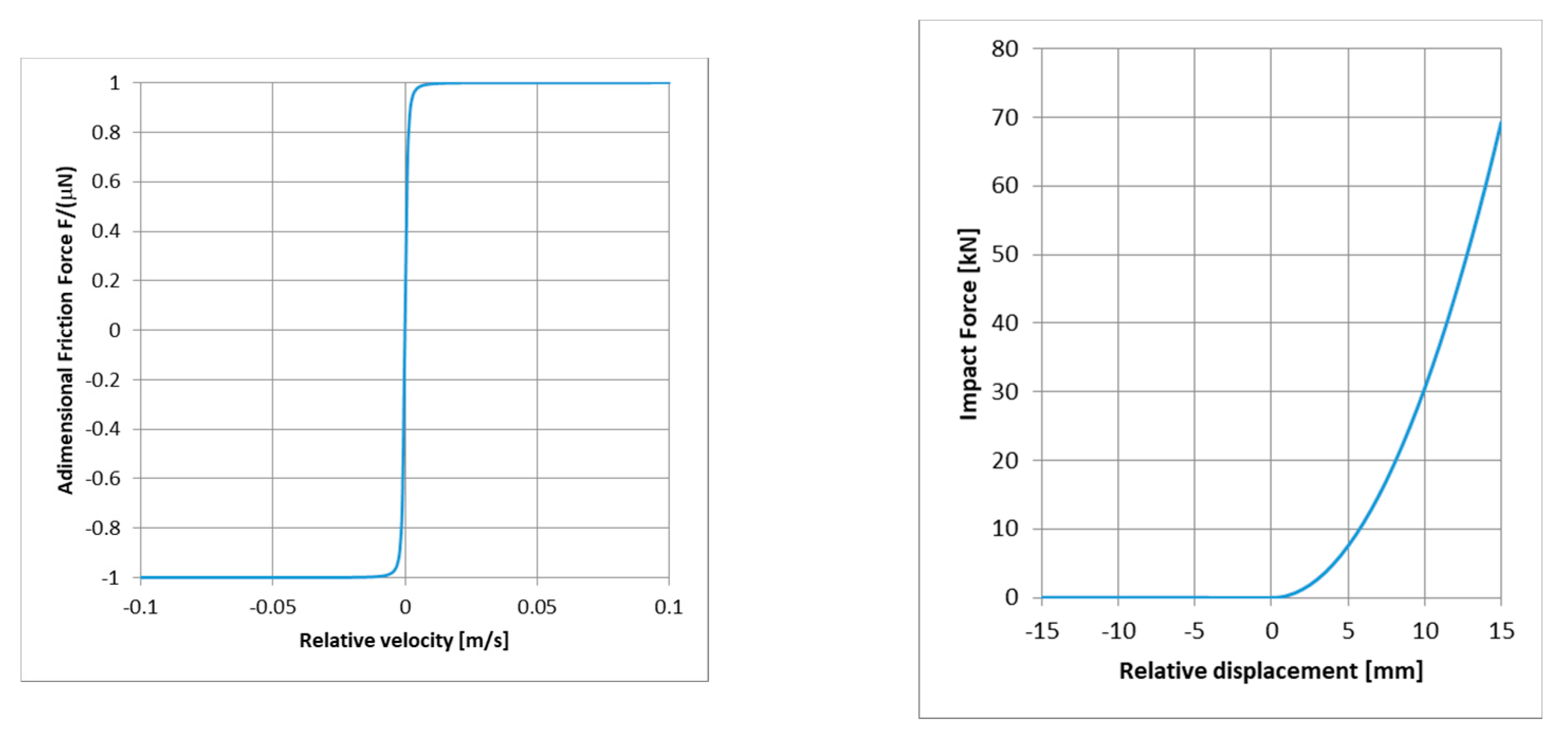
The function fimpact (x) represents an impact with a metallic surface; it has been defined according to Equation (4) and is plotted in Figure 3 on the right.

$$fimpact\left(x\right)=\left\{\begin{array}{ll}0& if\hspace{1em}x>0\\ 5·{10}^8·x^3+3·{10}^8·x^2-2·{10}^7·x& if\hspace{1em}x\le 0\end{array}\right.$$

(4)

D_i represents the damping, mainly due to the sliding of the piston in its seat, and is assumed as viscous and constant and equal to 10 Ns/m.

Both friction forces are applied between axle-box and bogie frame on the axis of action of the piston at a longitudinal coordinate corresponding to the considered friction surface on the axle-box. These forces are defined by Equations (5)–(8).

$$F_{Z\mu B,1}=-\mu ·F_{XP}·freg\left(V_1\right)·sin\left(\alpha \right)$$

(5)

$$F_{Z\mu B,2}=-\mu ·F_{XR}·freg\left(V_2\right)·sin\left(\alpha \right)$$

(6)

$$F_{Y\mu B,1}=-\mu ·F_{XP}·freg\left(V_1\right)·cos\left(\alpha \right)$$

(7)

$$F_{Y\mu B,2}=-\mu ·F_{XR}·freg\left(V_2\right)·cos\left(\alpha \right)$$

(8)

where μ is the friction coefficient, V_i is the relative velocity of the bogie frame with respect to the considered axle-box in the contact surface, and freg(V_i) is a function designed to regularize the Coulomb law and defined by a cubic spline. The regularized Coulomb law is plotted in Figure 3 on the left. This function assumes a value between −1 and 1 and has a unit value for a speed higher than 0.01 m/s, while for smaller values, the function behaves linearly (around the origin) and then assumes a non-linear trend.

This case corresponds to a two-dimensional friction; therefore, it is necessary to define the relative velocity between the friction surfaces according to Equation (9).

$$V_i=\sqrt{{\left({\dot{z}}_i^{+}\right)}^2+{\left({\dot{y}}_i^{+}\right)}^2}$$

(9)

where the subscript I indicates the surface of the piston (I = 1) or the paired surface on the opposite side of the axle-box (I = 2). The friction force is then decomposed again in the two directions by the angle α defined by the two relative speeds and calculated according to Equation (10).

$$tan\left(\alpha \right)=\frac{{\dot{z}}^{+}}{{\dot{y}}^{+}}$$

(10)

The vertical force between the axle-box and the bogie frame has been calculated by means of two shear-spring elements, included in the Simpack library [20] and defined by means of linear stiffness in the horizontal (XY) plane (transversal direction), three linear torsional stiffnesses, and a non-linear stiffness in the vertical (Z) direction. A spline function has been used for this direction, which expresses the non-linearity due to the intervention of the internal spring after a certain load. The stiffness parameters for 22.5 ton/axle bogie of each pair of springs are shown in

Table 2. Stiffness of primary suspension (per group) for 22.5 ton/axle bogie.

Direction	Stiffness	Unit
Kx	589	[N/mm]
Ky	589	[N/mm]
Kxx	1000	[Nmm/rad]
Kyy	1000	[Nmm/rad]
Kzz	0	[Nmm/rad]
Kz1 1	300	[N/mm]
Kz2 2	1216	[N/mm]

¹ Tare stiffness, ² Load stiffness.

. The primary suspension stiffness is modified when higher axle loads are considered, as described in the following sections.

2.3. Secondary Suspension

The secondary suspension consists of a spherical center plate placed at the center of the bogie and two side-bearers mounted on the two outer sides of the bogie frame, at a distance of 1700 mm, as shown in Figure 4.

The car body is fixed to the upper part of the center plate and each side-bearer is in contact with the lower surface of the car body (not represented in the figure) with an initial preload provided by a couple of helical springs (whose stiffness is shown in

Table 3. Stiffnesses of the secondary suspension.

Element	Direction	Stiffness	Unit
Center plate	Kx, Ky	100	[kN/mm]
	Kz	46	[kN/mm]
	Dx,Dy	1000	[Ns/m]
	Dz	400	[Ns/m]
	Dxx,Dyy,Dzz	Non-linear expression
Side-bearer	Kx, Ky	380	[N/mm]
	Kz	570	[N/mm]
	Kz (bumpstop)	100	[kN/mm]
	Dy	38	[Ns/m]
	Dz	57	[Ns/m]
	Dx	Non-linear expression

).

The preload of the side-bearer is adjusted so that it supports 25% of the load in tare condition; for the other load conditions, the load repartition between side-bearers and center plate depends on their stiffnesses.

The spherical center plate was modeled by a compact element (Bushing) characterized by linear axial stiffness, no rotational stiffness, and a frictional rotational damping that was introduced by an explicit function of the angular velocity.

Table 3 shows the stiffness and damping values adopted for the elements (Bushing type) used to simulate the center plate and the side-bearers. A metallic contact has been considered and simulated with an increased stiffness value, occurring after a vertical deflection of 12 mm of the surface of the side-bearer.

The torque due to friction damping of the center plate was calculated according to Equation (11).

$$T_{\mu ,j}=-{\mu }_{plate}·F_{plate}·R_{plate}·freg\left({\omega }_j\right) with\; j\; =\; 1,\; 2,\; 3.$$

(11)

where the index j indicates the axis considered, $R_{plate}$ represents the radius of the spherical joint, ${\mu }_{plate}$ the coefficient of friction of the center plate (0.6 is assumed according to data coming from field tests), and $F_{plate}$ is the resulting force acting on the center plate, calculated at each time step by the code.

The frictional force acting on the side-bearers has been instead calculated according to Equation (12).

$$F_{\mu ,sideb}=-{\mu }_{sideb}·F_{Z,sideb}·freg\left(V_x\right)$$

(12)

where $V_x$ expresses the relative velocity in the x direction between the side-bearer and the vehicle body frame, $F_{Z,sideb}$ is the vertical force acting on the side-bearer, and ${\mu }_{sideb}$ is the friction coefficient that has been adopted (0.7).

2.4. Wheel–Rail Contact Model

The contact model has been developed adopting the model implemented on Simpack [20], which consists of a rigid coupling of the profiles (using the quasi-elastic approach for the regularization of the constraint functions) and solving the problem of tangential forces using Kalker’s FASTSIM algorithm [21], although several other algorithms exist and can be implemented in Simpack, including the authors’ research group fast heuristic contact model [22].

New profiles are used to describe wheel and rail surfaces: S1002 for the wheels and UIC60 with a cant inclination 1:20 for the rails.

A constant wheel rail friction coefficient of 0.4 is adopted for all the simulations, and no degraded adhesion or adhesion recovery phenomena are considered [23,24,25].

2.5. Simulation of the Traction Effort

In order to control the speed of the vehicle, a tractive force, which simulates the actions of the hook-buffers device, is applied to the vehicle body at a height of 1060 mm. This force is applied between a marker defined on the coach and a “Follow-Track” marker defined on the ground. This last marker is a specific Simpack marker which is located and oriented according to the position and orientation of a specific body, in this case, the coach. This strategy guarantees that the traction force is always oriented parallel to the track. The force has been defined in Simpack by means of the expression shown in Equation (13), where Cp is a proportional constant (in this case equal to 20 kNs/m), V_ref is the reference vehicle speed, and V_vehicle is the actual velocity of the vehicle measured on the coach joint.

$$F_{traction}=Cp·\left({\mathrm{V}}_{ref}-V_{vehicle}\right)$$

(13)

The results shown in this paper are obtained keeping the vehicle speed constant during the simulations and starting the vehicle with an initial speed equal to the reference velocity. In this case, the traction is only required to overcome the resistance forces due to friction (rolling resistances), curves, and track slopes; thus, air brake forces [26] are neglected. A further step of this work could be running longitudinal train dynamic simulations of a reference train composition considering complex operations with traction and braking to compute more accurate values of the in-train forces [27,28]. The detailed simulation of the traction effort is very important to evaluate the impact of the vehicle in terms of wheel and rail wear and RCF risk. This aspect is neglected in this work, whose aim is to evaluate the possibility of increasing the axle load in terms of the parameters considered by the EN14363 homologation standard.

3. Track Model

The track was chosen considering a newly built real line of class D4 (22.5 t/axle), characterized by large radius curves and built with UIC60 rails and heavy armament. For the purpose of this paper, an existing good-quality section of track was chosen to analyze the impact of an increased axle load on the line according to the speed of the rolling stock, without any additional overload due to the presence, for example, of reduced radius curves.

This analysis therefore constitutes a reasonable initial verification of the feasibility of an increase in axle load on Italian lines.

Table 4. Characteristics of the planimetric layout.

Section	Type	Length [m]	Rinitial [m]	Rend [m]	SPinitial [mm]	SPend [mm]
1	Straight	220	-	-	-	-
2	Clothoid	60	0	2295.7	0	60
3	Circular	173	2295.7	2295.7	60	60
4	Clothoid	60	2295.7	0	60	0
5	Straight	130.52	-	-	-	-
6	Clothoid	60	0	−2403.3	0	−41.2
7	Circular	41.245	−2403.3	−2403.3	−41.2	−41.2
8	Clothoid	60	−2403.3	0	−41.2	0
9	Straight	1627.18	-	-	-	-
10	Clothoid	44	0	−45,000	0	−43.8
11	Circular	44	−45,000	−45,000	−43.8
12	Clothoid	44	−45,000	0	−43.8	0
13	Straight	2283.91	-	-	-	-
14	Clothoid	330	0	−6002.15	0	−35
15	Circular	488.599	−6002.15	−6002.15	−35	−35
16	Clothoid	330	−6002.15	0	−35	0
17	Straight	1791.52	-	-	-	-
18	Clothoid	330	0	5997.85	0	35
19	Circular	4041.59	5997.85	5997.85	35	35
20	Clothoid	330	5997.85	0	35	0
21	Straight	1460.41	-	-	-	-
22	Clothoid	330	0	5997.85	0	35
23	Circular	2592.23	5997.85	5997.85	35	35
24	Clothoid	330	5997.85	0	35	0
25	Straight	127.5	-	-	-	-
26	Clothoid	52	0	−4502	0	−45
27	Circular	371.33	−4502	−4502	−45	−45
28	Clothoid	52	−4502	0	−45	0
29	Straight	672.21	-	-	-	-
30	Clothoid	174	0	1250	0	150
31	Circular	76.37	1250	1250	150	150
32	Clothoid	174	1250	0	150	0

shows the nominal characteristics of the considered line; in addition, a set of plano-altimetric, rolling, and gauge irregularities was adopted. Track irregularities were simulated by means of defects generated with a spectrum of irregularities corresponding to the ORE standard for low defects [29] and superimposed to the theoretical track described by Table 4.

Track irregularities were introduced in Simpack by using the ERRI spectra for small defects already included in the code library. The irregularities are defined as track-related considering lateral, vertical, roll, and gauge direction. The ERRI B176 [29] does not define a gauge excitation but it is a common approach to adopt the crosslevel spectrum for this direction. The range of distance frequencies where the spectra are valid is not indicated by the ERRI, and in this work it has been adopted in the range 0.04 m⁻¹ – 0.333 m⁻¹, which corresponds to the typical measurement range of track measurement systems. In particular, the numerical model considers 500 distance frequencies inside this range.

It is evident that the approach used leads to the estimation of dynamic loads on the vehicle and on the infrastructure that are substantially linked to a good-quality track layout and to the particular type of irregularities that were chosen. A spectrum corresponding to “small defects” was used, but the simulations carried out cannot take into account the presence of major discontinuities of the track (switches, joints) that are presumably present in a real track. The simulation of the vehicle behavior in such circumstances and the strategies to be adopted during the exercise (for example, speed reduction) must necessarily be evaluated case by case through ad hoc studies.

For the layout of the track, a rigid track model was used; it provides that the rails are fixed rigidly to the sleeper but allows three degrees of freedom to the sleeper (vertical, lateral, and roll), which is connected to the ballast (rigid body) by means of elastic elements. This approach is commonly used in the literature [30,31], and it is suitable to simulate the general dynamic behavior of the vehicle considering track excitation in the spatial frequency range considered for this simulation.

In [31], a FEM model of the track is compared to a sectional model (corresponding to the model adopted in this work) and a difference of less than 7% is found on the critical speed, while the behavior of the track contact forces is quite similar up to 20 Hz. Obviously, the model is not able to reproduce accurately local phenomena (track joints, wheel flats, etc.), whose dynamic excitation operates at high frequency. Furthermore, the proposed model is stiffer than the real track at high frequency and the simulated loads are expected to be higher than in reality.

A vertical stiffness of 75 kN/mm, a lateral stiffness of 20 kN/mm, a rolling stiffness of 84 kNm/rad, and a mass of the sleeper of 330 kg were considered.

Table 4 shows the curvatures on the horizontal plane at the beginning and at the end of the section (R_initial, R_end if there is a variation) and the superelevation (SP_initial, SP_end) given to the inner rail in curve.

Table 5. Track altimetry.

Section	Type	Length [m]	Pinitial [‰]	Pend [‰]	Pconstant [‰]
1	Constant	556.25	-	-	0.14
2	Circular	50.6	0.14	5.20	-
3	Constant	217.44	-	-	5.20
4	Circular	21.5	5.20	4.77	-
5	Constant	736.51	-	-	4.77
6	Circular	112.9	4.77	8.00	-
7	Constant	3472.95	-	-	8.00
8	Circular	431.44	8	−2.79	-
9	Constant	2692.27	-	-	−2.79
10	Circular	276.3	−2.79	−11.99	-
11	Constant	496.3	-	-	−11.99
12	Circular	804.02	−11.99	4.08	-
13	Constant	479.93	-	-	4.08
14	Circular	592.8	4.082	−7.78	-
15	Constant	433.85	-	-	−7.78
16	Circular	413.38	−7.77	0.49	-
17	Constant	817.7	-	-	0.49
18	Circular	375.24	0.49	8	-
19	Constant	2005.02	-	-	8
20	Circular	618.14	8	−4.37	-
21	Constant	111.37	-	-	−4.37
22	Circular	222.8	−4.37	3.07	-
23	Constant	463.61	-	-	3.07
24	Circular	231.44	3.07	−4.67
25	Constant	532.13	-	-	−4.67
26	Circular	8.42	−4.67	−4.71	-
27	Constant	542.94	-	-	−4.71
28	Circular	264.56	−4.71	−11.88	-
29	Constant	857.3	-	-	−11.88

shows the track altimetry, including the section with constant gradient (P_constant) and slope variations that are realized with circular crossings.

4. Design of the Primary Suspension for Higher Axle Load

In order to be able to carry out analysis with higher axle load that is realistic, it is necessary to redesign the primary suspension of the vehicle. In particular, the stiffness of the primary springs is modified in such a way as to keep the vertical frequency of the vehicle constant as the axle load increases. The primary suspension consists of the tare stage which is placed in parallel to the load stage. The latter acts only after the tare stage has undergone a pre-set deflection. In accordance with the standards [32], it was decided to consider a tare frequency f_Tare equal to 3.5 Hz and a full load frequency f_Load equal to 2.5 Hz. The stiffnesses of the individual springs that compose the primary suspension are calculated using the Equations (14) and (15).

$$K_{z,Tare}=\frac{1}{2}{\left(2\pi f_{Tare}\right)}^2·\left(\frac{P_{axle,Tare}-M_{wheelset}}{2}\right)$$

(14)

$$K_{z,Load}=\frac{1}{2}{\left(2\pi f_{Load}\right)}^2·\left(\frac{P_{axle,Load}-M_{wheelset}}{2}\right)-K_{z,Tare}$$

(15)

In Equations (14) and (15), P_axle,Tare and P_axle,Load are, respectively, the axle loads corresponding to the tare and full load conditions, while M_wheelset is the mass of the wheelset and axle-boxes (unsprung masses).

Table 6. Calculation of the primary suspension nominal stiffness.

Paxle,Tare [ton/axle]	Paxle,Load [ton/axle]	Mwheelset [ton]	fLoad [Hz]	fTare [Hz]	Kz,Load [kN/mm]	Kz,Tare [kN/mm]
5.18	25.00	1.47	3.50	2.50	1.14	0.45
5.35	27.50	1.52	3.50	2.50	1.28	0.46
5.50	30.00	1.56	3.50	2.50	1.42	0.48
5.65	32.50	1.61	3.50	2.50	1.56	0.49
5.79	35.00	1.65	3.50	2.50	1.14	0.50

shows the nominal values of the stiffnesses of the suspensions corresponding to the different axle loads.

Once the nominal stiffnesses have been calculated, the coil springs that compose the primary suspension are designed.

Table 7. Mechanical characteristics of the tare helical spring.

Paxle,Load [ton/axle]	Active Turns N	Mean Diameter D [mm]	Wire Diameter d [mm]	Effective Stiffness Kz,Tare [kN/mm]	Variation from Nominal Stiffness %	Free Length L0 [mm]	Total Turns Ntot	Solid Length [mm]
25.00	4.0	169.0	31.0	0.48	6.5	261	5.5	170.5
27.50	4.0	169.0	31.0	0.48	3.2	266	5.5	170.5
30.00	4.5	168.0	32.0	0.49	3.0	300	6.0	192.0
32.50	4.5	168.0	32.0	0.49	0.2	300	6.0	192.0
35.00	4.5	167.5	32.5	0.53	5.0	305	6.0	195.0

shows the main mechanical characteristics of the tare coil spring.

Table 8. Mechanical characteristics of the load helical spring.

Paxle,Load [ton/axle]	Active Turns N	Mean Diameter D [mm]	Wire Diameter d [mm]	Effective Stiffness Kz,Load [kN/mm]	Variation from Nominal Stiffness %	Free Length L0 [mm]	Total Turns Ntot	Solid Length [mm]
25.00	5.0	94.5	25.5	1.00	−0.3	228.0	6.5	165.8
27.50	5.0	93.5	26.5	1.20	5.6	225.0	6.5	172.3
30.00	5.5	92.5	27.5	1.31	2.6	252.0	7.0	192.5
32.50	5.5	92.0	28.0	1.43	1.1	253.0	7.0	196.0
35.00	5.0	92.0	28.0	1.58	1.3	257.0	6.5	182.0

, on the other hand, shows the mechanical characteristics of the loading spring. The axial stiffness of the spring was calculated according to Equation (16), where G is the shear modulus of the steel (about 80 Gpa).

$$K_z=\frac{G{d}^4}{8N{D}^3}$$

(16)

In order to carry out the structural analysis of the spring, it is necessary to calculate the force acting on the tare spring and on the load spring when the vehicle is in the full load condition. Since the action of the load spring takes place only after a certain deflection of the tare spring, it is first necessary to calculate the mass M_int which causes the action of the load spring; see Equation (17).

$$M_{int}=\frac{K_{z,Tare}\left(L_{0,Tare}-L_{0,Load}\right)}{g}$$

(17)

The corresponding P_int axle load that causes the action of the load spring can be calculated using Equation (18). The multiplication factor four corresponds to the number of tare springs acting on each axle (two per axle-box).

$$P_{int}=4M_{int}$$

(18)

The vertical frequency of the vehicle when the load spring is involved can be calculated according to Equation (19).

$$f_{int}=\frac{1}{2\pi }\left(\sqrt{4\frac{K_{z,Tare}+K_{z,Load}}{P_{int}}}\right)$$

(19)

After the action of the full load spring, the tare and full load springs work in parallel and undergo the same deflection Δl, which can be calculated using Equation (20).

$$\mathsf{\Delta }l=\frac{P_{axle,Load-M_{wheelset}-P_{int}}}{4\left(K_{z,Tare}+K_{z,Load}\right)}$$

(20)

Knowing the deflection Δl of the suspension in full load condition, the load exerted by each spring can be determined; see Equations (21) and (22).

$$F_{z, Tare}=K_{z,Tare}\left(L_{0,Tare}-L_{0,Load}+\mathsf{\Delta }l\right)$$

(21)

$$F_{z, Load}=K_{z,Load}\mathsf{\Delta }l$$

(22)

The maximum stress acting on the spring can be calculated according to Equation (23).

$${\tau }_{max}=k_w\frac{8F_{z}D}{\pi d^3}$$

(23)

Wahl factor k_w as a function of the C = D/d ratio can be calculated according to Equation (24).

$$k_w=\frac{4C-1}{4C-4}+\frac{0.615}{C}$$

(24)

Assuming a material with allowable tangential stress τ_adm of 1040 Mpa. it is possible to determine the safety factor SF of the spring using Equation (25).

$$SF=\frac{{\tau }_{adm}}{{\tau }_{max}}$$

(25)

Table 9. Safety factors calculation for helical springs.

Paxle,Tare [ton/axle]	Paxle,Load [ton/axle]	Mwheelset [ton]	Pint [ton]	fint [Hz]	L0,Tare − L0,Load + Dl [mm]	Dl [mm]	tMax Tare Spring [MPa]	tMax Load Spring [MPa]	SF Tare Spring	SF Load Spring
5.18	25.00	1.47	6.42	4.83	61.4	28.4	542	595	1.92	1.75
5.35	27.50	1.52	7.98	4.62	67.3	26.3	594	595	1.75	1.75
5.50	30.00	1.56	9.60	4.36	73.6	25.6	610	571	1.70	1.82
5.65	32.50	1.61	9.40	4.55	74.4	27.4	616	635	1.69	1.64
5.79	35.00	1.65	10.31	4.55	74.9	26.9	637	685	1.63	1.52

summarizes the structural analysis of tare and load springs.

5. Simulations and Results

In order to analyze the effect of an increase in axle load in relation to the vehicle speed, simulations were carried out at two different velocities, 80 and 120 km/h. The axle load of the vehicle was changed from 22.5 tonnes to 35 tonnes with a step of 2.5 tonnes.

The results of the simulations were statistically analyzed according to the indications of the Fiche UIC 518 [33] and the EN14363 standard [34].

In particular, this work considers the dynamic vertical load Q on the track, the total forces acting on the wheelset in the lateral direction ΣY, the derailment safety ratio for wheel running on the outer rail Y/Q (limit value of 0.8 according to both EN14363 and UIC 518), the lateral accelerations measured in the vehicle frame (limit value of 3 m/s² according to both EN14363 and UIC 518), and the vertical accelerations measured in the vehicle frame (limit value of 5 m/s² according to both EN14363 and UIC 518). As regards total forces acting on the wheelset ΣY, the limit depends on the vehicle mass and it can be calculated according to Equation (26) (EN14363), where Q₀ is the nominal wheel load in kN, or according to Equation (27) (UIC518), where P₀ is the nominal axle load in kN.

$$\mathsf{\Sigma }\mathrm{Y}=0.85·\left(10+\frac{2{\mathrm{Q}}_0}{3}\right)$$

(26)

$$\mathsf{\Sigma }\mathrm{Y}=0.80·\left(10+\frac{{\mathrm{P}}_0}{3}\right)$$

(27)

The limits considering an axle load of the vehicle of 22.5 t, 25 t and 35 t are, respectively, equal to 71, 78, and 106 kN according to EN14363, and equal to 67, 73, and 100 kN according to UIC 518.

The data simulated numerically by the multibody model and sampled at 200 Hz, have been processed considering sections of 100 m in length, on each of which the percentiles of the quantities of interest have been calculated. The results obtained at 80 km/h are shown in graphical form (Figure 5, Figure 6, Figure 7, Figure 8, Figure 9 and Figure 10) for two different axle loads (22.5 and 35).

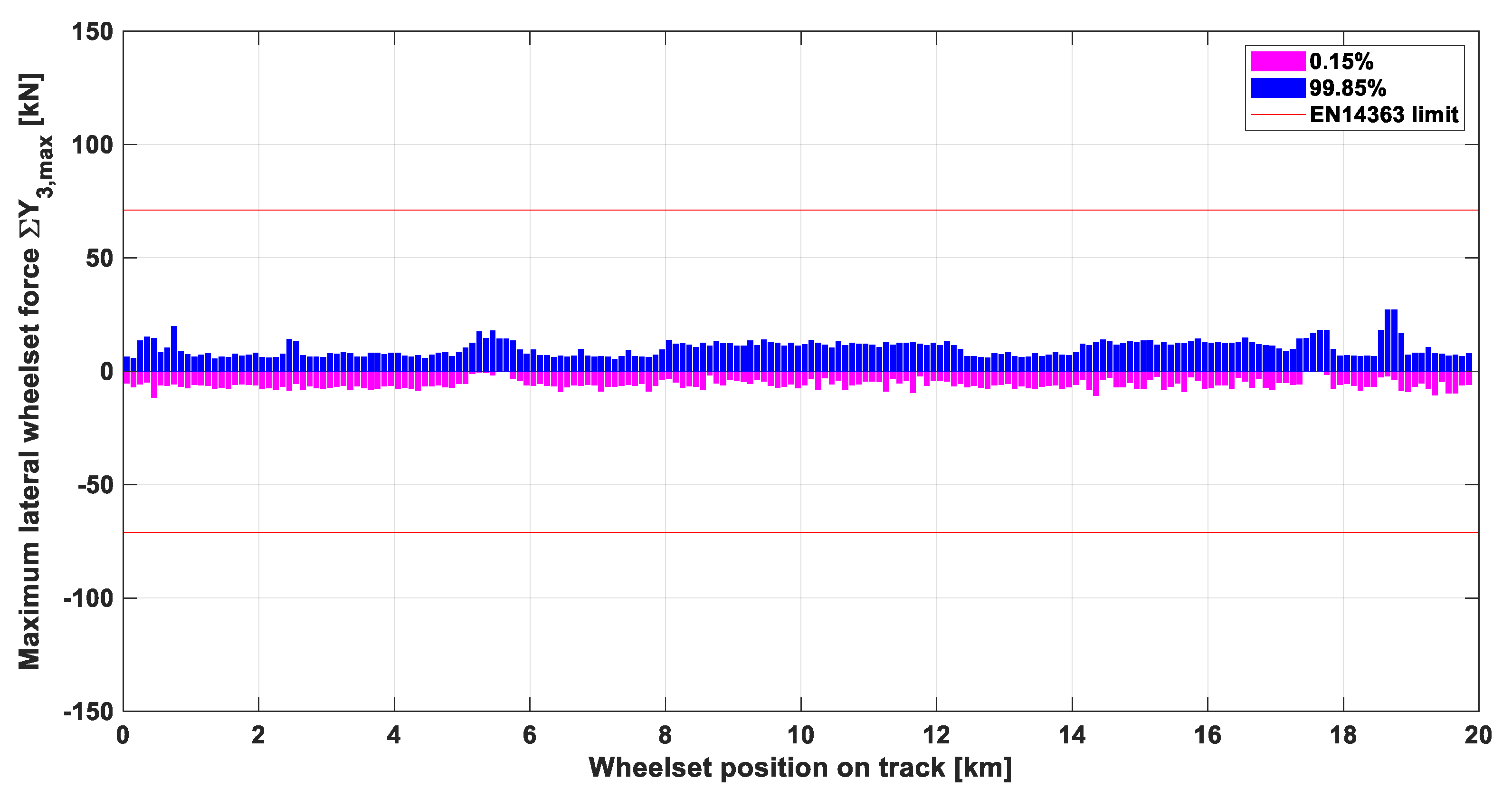
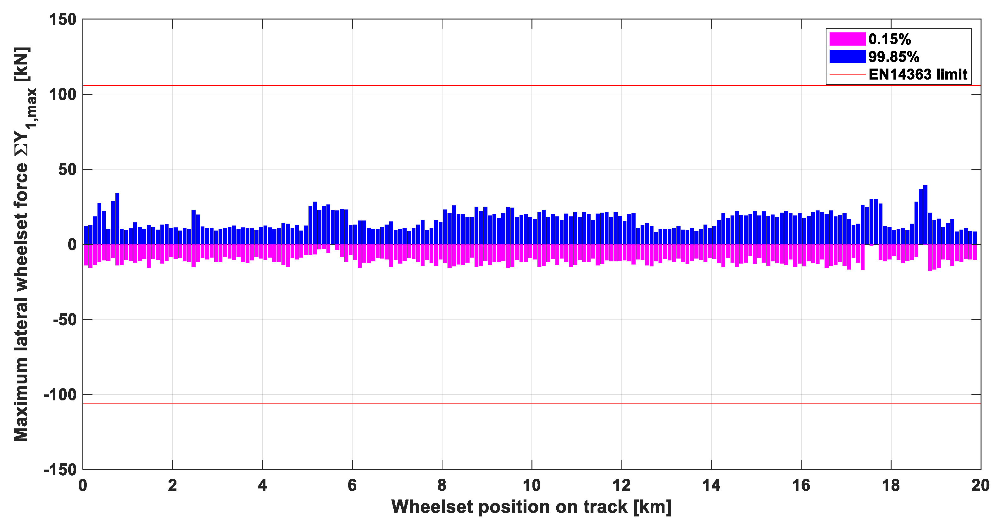
Figure 5 and Figure 6 show the lateral forces acting between the wheelset and the track (for the leading wheelset) considering the two different axle loads. For each 100 m length section, the percentiles at 99.85% and 0.15% of the filtered value of the sum of the lateral forces on the wheelset are considered. The forces are filtered by means of a low-pass filter with a cut-off frequency of 20 Hz (Chebyshev 3dB), and then by a moving average with a sampling interval of 0.5 m over a reference distance of 2 m.

The two lines in red show the limits set by the EN14363 standard for the lateral forces (ΣY); it is possible to observe that in the considered path (large radius curves), the vehicle is very far from the limit value.

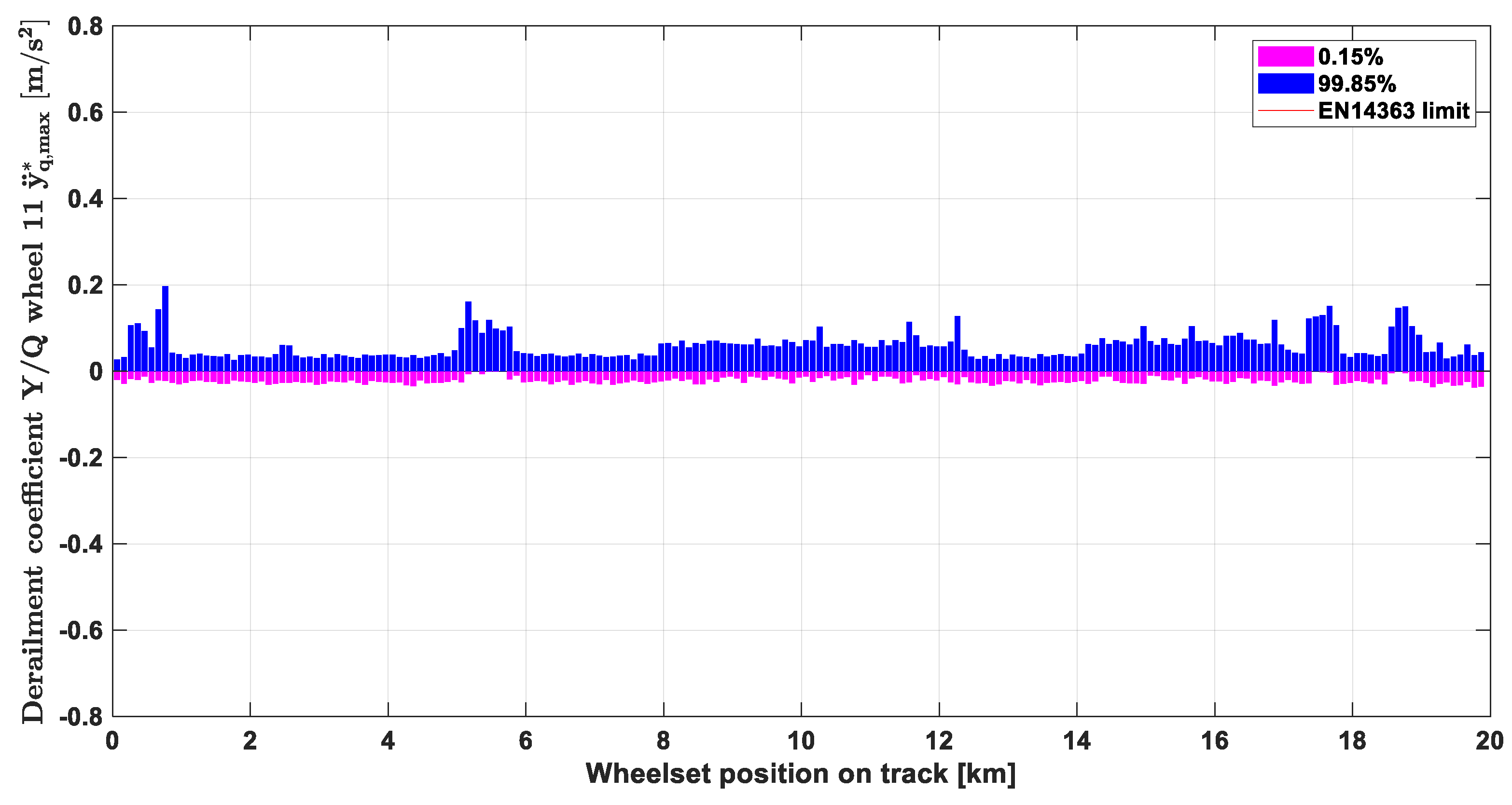
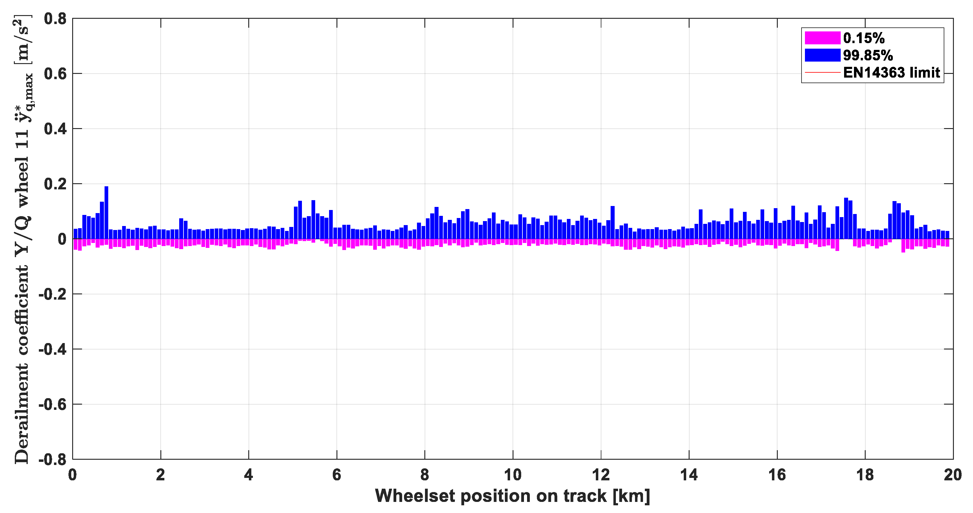
Figure 7 and Figure 8 show the values of the derailment safety ratio Y/Q; also in this case, the data obtained from the simulations are filtered in the same mode of the Y forces, as required by the standard, and were considered the percentiles at 99.85% and at 0.15%. The limit value (0.8) is well respected.

Finally, Figure 9 and Figure 10 show the vertical force on each section of the track acting on the leading wheelset of the vehicle for the case of 22.5 t and 35 t per axis. In this case, the simulation data are filtered at 20 Hz and the 99.85% percentile was considered on each 100 m segment.

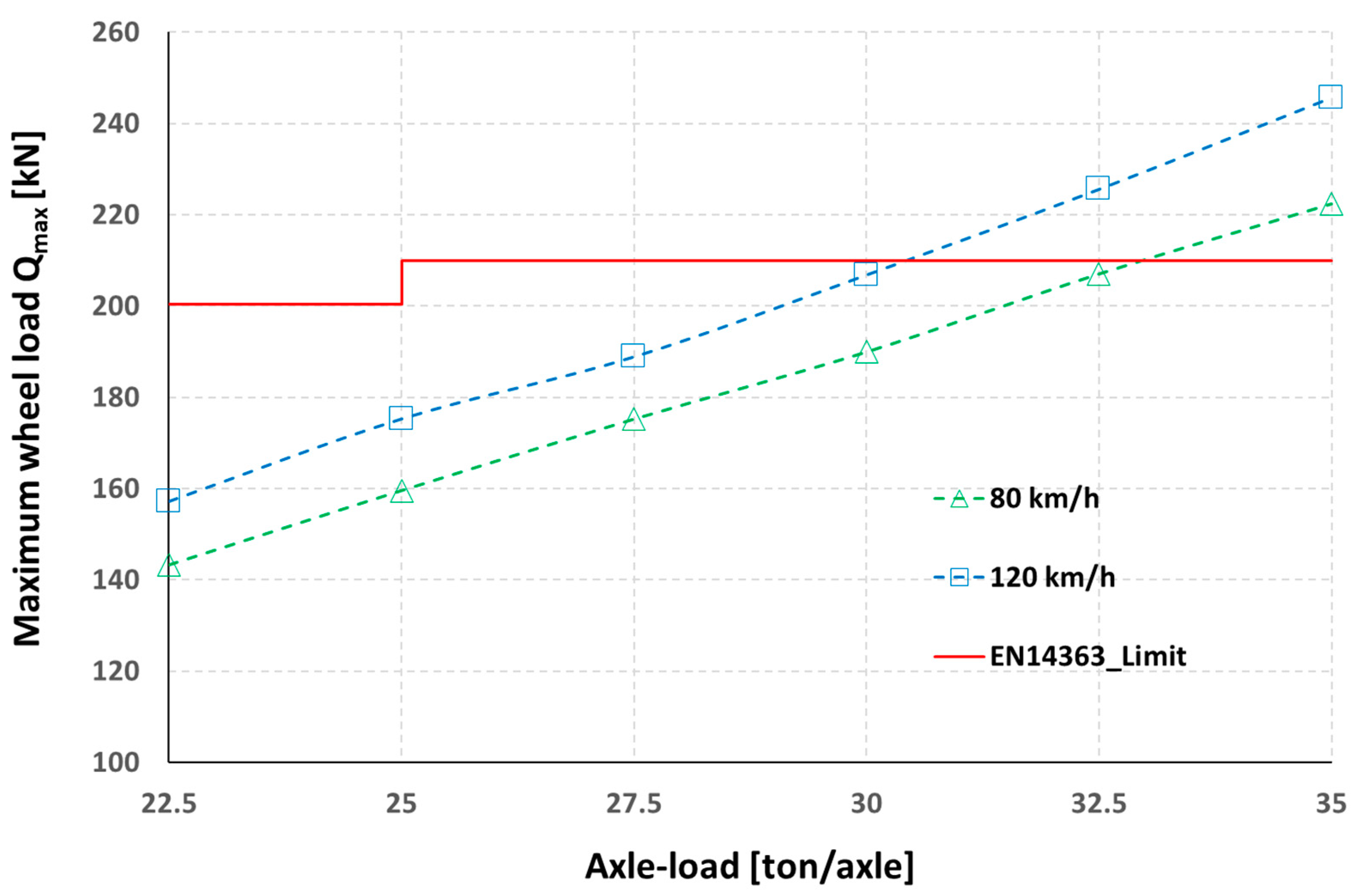
As shown in the diagrams, in the case of 22.5 t per axle, the limit is respected with a good safety margin. In the case of 35 t per axle, the limit load is exceeded by about 5%.

The summary of the results obtained is illustrated in

Table 10. Summary of results at 80 km/h.

Quantity	Axle Load [tonnes]
	22.5	25	27.5	30	32.5	35
ΣY [kN]	27	30	34	36	39	39
Y/Q [/]	0.20	0.20	0.19	0.15	0.20	0.19
${\ddot{y}}^{*}$ [m/s2]	0.94	0.85	0.83	0.80	0.85	0.88
${\ddot{z}}^{*}$ [m/s2]	0.77	0.69	0.68	0.59	0.75	0.81
Q [kN]	143	160	175	190	207	222
Q0 [kN]	110	122.5	135	147	159.5	171.5
(Q-Q0)/Q0 [%]	30	30	30	29	30	30

and

Table 11. Summary of results at 120 km/h.

Quantity	Axle Load [tonnes]
	22.5	25	27.5	30	32.5	35
ΣY [kN]	34	39	44	43	50	47
Y/Q [/]	0.23	0.23	0.23	0.23	0.22	0.22
${\ddot{y}}^{*}$[m/s2]	1.36	1.50	1.52	1.43	1.41	1.38
${\ddot{z}}^{*}$[m/s2]	1.33	1.35	1.39	1.41	1.57	1.58
Q [kN]	157	175	189	207	226	246
Q0 [kN]	110	122.5	135	147	159.5	171.5
(Q-Q0)/Q [%]	43	43	40	41	42	43

(80 km/h and 120 km/h). The tables show the maximum values measured on the entire section considered and reprocessed according to the methodology proposed by EN14363.

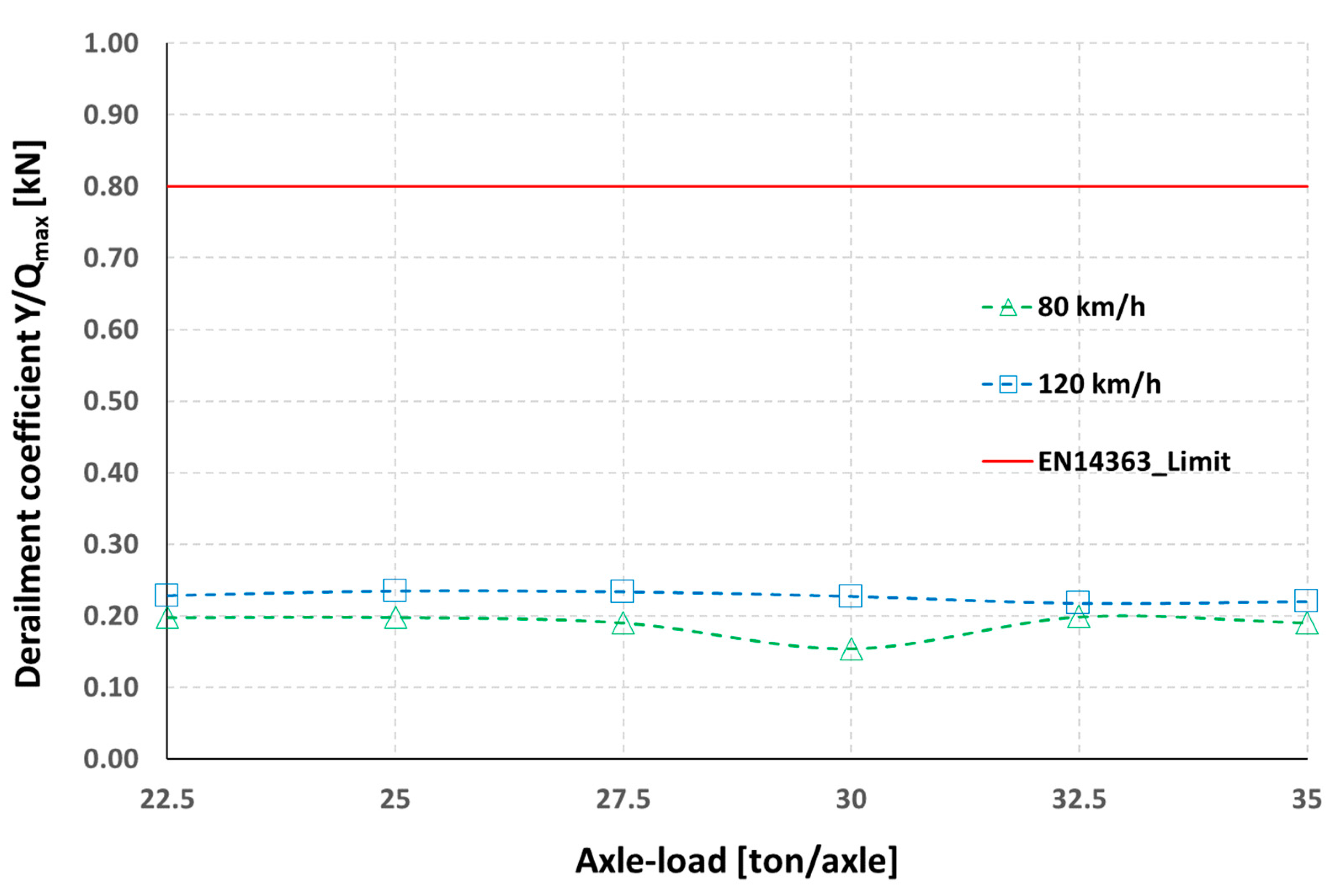
Analyzing the results, shown in Figure 11, Figure 12, Figure 13, Figure 14 and Figure 15, the most critical parameter is the vertical load, which at 35 t per axis exceeds the limit proposed by EN14363 for speeds both of 80 km/h and 120 km/h. The limit is also exceeded for a speed of 120 km/h when considering an axle load of 32.5 t. The lateral forces, the derailment coefficient, and the accelerations in the vehicle body are instead always lower than the limits proposed by the EN14363 standard.

It is particularly interesting to note that the difference between the maximum load on the rail and the static load is not a function of the axle load. This means that as the load increases, the effect of the dynamic on the vertical forces is constant. This aspect highlights in the preliminary stage good prospects for the use of freight wagons with increased load compared to the actual limit.

6. Conclusions

The study proposed in this paper proves that the increase of the axle load for European wagons is in the first analysis sustainable. In particular, the results show that an increase in the axle load is possible until an axle load of 32.5 ton if speed is limited to 80 km/h, or until 30 ton if speed is limited to 120 km/h. The evaluations were limited to new construction lines with good plano-altimetric characteristics (large radius curves, optimal transitions); in particular, the analyses were performed considering a real track layout.

In order to obtain realistic indications, track irregularities were considered on the theoretical track, corresponding to a state of standard wear of the track.

In addition, in this condition is highlighted how it is possible to increase the axle load, even in a relevant way, while still remaining within the limits set by the regulations. Further improvement margins will be possible by optimizing the suspension of the rolling stock for the axle load considered.

It should be noted that the study here illustrated should be further extended considering the effects on contact pressure, which in the case of Italian cant (1:20), is penalizing with new profiles.

Finally, it should be noted that further aspects to be considered in future analysis, which have not been examined here, are related to the braking of trains and more generally to the operation in terms of blocking and signaling sections, and to the structural strength of the wagon. For this last aspect, the considerations concerning the reduction of the effects of dynamic loads with increasing axle load appear to be promising.

References

- European Commission. WHITE PAPER Roadmap to a Single European Transport Area—Towards a Competitive and Resource Efficient Transport System; COM: Brussels, Belgium, 2011; pp. 1–144.
- LoPresti, J.; Kalay, S. The 35-Tonne Heavy Axle Load Testing Continues at FAST. Available online: http://www.ihha.net/articles/the-35-tonne-heavy-axle-load-testing-continues-at-fast (accessed on 15 January 2023).
- Harder, R.F. Dynamic modeling and simulation of three-piece freight vehicle suspensions with non-linear frictional behaviour using ADAMS/Rail. In Proceedings of the IEEE/ASME Joint Railroad Conference 2001, Toronto, ON, Canada, 19 April 2001. [Google Scholar]
- Sun, Y.Q.; Cole, C. Comprehensive wagon-track modelling for simulation of three-piece bogie suspension dynamics. Proc. Inst. Mech. Eng. Pt. F J. Rail Rapid Transit 2007, 221, 905–917. [Google Scholar] [CrossRef]
- Hu, L.; Yang, J.; Feng, D.; Zhang, L.; Xiao, F. Research on the Key Design Parameters of Sleeper for 40 t Axle-load Heavy Haul Railway. J. Railw. Eng. Soc. 2017, 34, 25–29. [Google Scholar]
- Zhang, D.; Zhai, W.; Wang, K. Dynamic interaction between heavy-haul train and track structure due to increasing axle load. Aust. J. Struct. Eng. 2017, 18, 190–203. [Google Scholar] [CrossRef]
- Orlova, A.M.; Saidova, A.V.; Rudakova, E.A.; Komarova, A.N.; Gusev, A.V. Advancements in three-piece freight bogies for increasing axle load up to 27 t. In Proceedings of the 24th Symposium of the International Association for Vehicle System Dynamics IAVSD 2015, Graz, Austria, 17–21 August 2015. [Google Scholar]
- Bosso, N.; Macaluso, D.; Salvo, G. Effetti dinamici dell’innalzamento del carico per asse di rotabili ferroviari per trasporto merci. In Proceedings of the 40° Convegno Nazionale AIAS, Palermo, Italy, 7–10 September 2011. [Google Scholar]
- ERRI. Dynamic Effects of 22.5 t Axle Load on the Track; Report D 161.1 Rp 1-4; Railway Technical Publications: Paris, France, 1987. [Google Scholar]
- ERRI. Increasing Axle Loads beyond 22.5 t for Wheels with a Diameter of 920 mm; Report B169.5; Railway Technical Publications: Paris, France, 1999. [Google Scholar]
- Jendel, T. Dynamic Analysis of a Freight Wagon with Modified Y25 Bogies; TRITAFKT Report 1997:48; KTH Railway Technology: Stockholm, Sweeden, 1997. [Google Scholar]
- Hossein Nia, S.; Jönsson, P.; Stichel, S. Wheel damage on the Swedish iron ore line investigated via multibody simulation. Proc. Inst. Mech. Eng. Pt. F J. Rail Rapid Transit 2014, 228, 652–662. [Google Scholar] [CrossRef]
- UIC. Complément à la Fiche UIC 518: Application aux Wagons de Charge à L’essieu Supérieure à 22,5 t et Jusqu’à 25 t; Fiche UIC 518-2; UIC: Paris, France, 2004. [Google Scholar]
- EN 15528:2008; Railway Applications. Line Categories for Managing the Interface between Load Limits of Vehicles and Infrastructure. European Committee for Standardization: Brussels, Belgium, 2008.
- European Commission. Commission Decision of 28 July 2006 Concerning the Technical Specification of Interoperability Relating to the Subsystem ‘Rolling Stock—Freight Wagons’ of the Trans-European Conventional Rail System. (2006/861/EC); European Commission: Brussels, Belgium, 2006.
- European Commission. Commission Regulation (EU) No 321/2013 of 13 March 2013 Concerning the Technical Specification for Interoperability Relating to the Subsystem ‘Rolling Stock—Freight Wagons’ of the Rail System in the European Union; European Commission: Brussels, Belgium, 2013.
- UIC. Classification of Lines—Resulting Load Limits for Wagons; Fiche UIC 700; UIC: Paris, France, 2004. [Google Scholar]
- Volker, G. Hydraulic Spring Used as Principal Spring in Rail Vehicles. European Patent EP1369616, 25 October 2006. [Google Scholar]
- Bosso, N.; Gugliotta, A.; Somà, A. Multibody simulation of a freight bogie with friction dampers. In Proceedings of the ASME/IEEE 2002 Joint Rail Conference, Washington, DC, USA, 23–25 April 2002. [Google Scholar]
- Simpack, A.G. Force Element Catalogue. Simpack Release 9.01: Munchen, Germany, 2009. [Google Scholar]
- Kalker, J.J. A Fast Algorithm for the Simplified Theory of Rolling Contact. Veh. Syst. Dyn. 1982, 11, 1–13. [Google Scholar] [CrossRef]
- Bosso, N.; Zampieri, N. A Novel Analytical Method to Calculate Wheel-Rail Tangential Forces and Validation on a Scaled Roller-Rig. Adv. Trib. 2018, 2018, 7298236. [Google Scholar] [CrossRef]
- Bosso, N.; Gugliotta, A.; Magelli, M.; Oresta, I.F.; Zampieri, N. Study of wheel-rail adhesion during braking maneuvers. Proc. Struct. Int. 2019, 24, 680–691. [Google Scholar] [CrossRef]
- Bosso, N.; Gugliotta, A.; Magelli, M.; Zampieri, N. Experimental Setup of an Innovative Multi-Axle Roller Rig for the Investigation of the Adhesion Recovery Phenomenon. Exp. Tech. 2019, 43, 695–706. [Google Scholar] [CrossRef]
- Bosso, N.; Magelli, M.; Zampieri, N. Investigation of adhesion recovery phenomenon using a scaled roller-rig. Veh. Syst. Dyn. 2021, 59, 295–312. [Google Scholar] [CrossRef]
- Wu, Q.; Cole, C.; Spiryagin, M.; Chang, C.; Wei, W.; Ursulyak, L.; Shvets, A.; Murtaza, M.A.; Zhelieznov, K.; Mohammadi, S.; et al. Freight train air brake models. Int. J. Rail. Transp. 2021, 1–49. [Google Scholar] [CrossRef]
- Bosso, N.; Magelli, M.; Zampieri, N. Development and validation of a new code for longitudinal train dynamics simulation. Proc. Inst. Mech. Eng. F J. Rail Rapid Transit. 2021, 235, 286–299. [Google Scholar] [CrossRef]
- Bosso, N.; Magelli, M.; Rossi Bartoli, L.; Zampieri, N. The influence of resistant force equations and coupling system on long train dynamics simulations. Proc. Inst. Mech. Eng. F J. Rail Rapid Transit. 2022, 236, 35–47. [Google Scholar] [CrossRef]
- ORE. Power Spectral Density of Track Irregularities. Part 1: Definitions, Conventions and Available Data; Question ORE C116-Rp1; International Union of Railways: Utrecht, The Netherlands, 1971. [Google Scholar]
- Andersson, C.; Abrahamsson, T. Simulation of interaction between a train in general motion and a track. Veh. Syst. Dyn. 2002, 38, 433–455. [Google Scholar] [CrossRef]
- Di Gialleonardo, E.; Braghin, F.; Bruni, S. The influence of track modelling options on the simulation of rail vehicle dynamics. J. Sound Vib. 2012, 331, 4246–4258. [Google Scholar] [CrossRef]
- EN 16235; Railway Application—Testing for the Acceptance of Running Characteristics of Railway Vehicles—Freight Wagons—Conditions for Dispensation of Freight Wagons with Defined Characteristics from On-Track Tests According to EN14363. European Committee for Standardization: Brussels, Belgium, 2013.
- UIC. Testing and Approval of Railway Vehicles from the Point of View of Their Dynamic Behaviour—Safety—Track Fatigue—Ride Quality; Fiche UIC 518; UIC: Paris, France, 2005. [Google Scholar]
- EN 14363:2016; Railway Applications—Testing and Simulation for the Acceptance of Running Characteristics of Railway Vehicles—Running Behaviour and Stationary Tests. European Committee for Standardization: Brussels, Belgium, 2016.
Figure 1.
Multibody model of the bogie assembled on the track.
Figure 2.
Primary suspension and Lenoir-Link device.
Figure 3.
Regularized Coulomb law (left), and impact function (right).
Figure 4.
Secondary suspension: cross-section of the bogie frame.
Figure 5.
Sum of lateral forces (ΣY) on the first wheelset of the second bogie, 22.5 t/axle, speed 80 km/h.
Figure 6.
Sum of lateral forces (ΣY), on the leading wheelset of the leading bogie, 35 t/axle, speed 80 km/h.
Figure 7.
Derailment safety ratio (Y/Q) of the right wheel of leading wheelset of first bogie, 22.5 t/axle, speed 80 Km/h.
Figure 8.
Derailment safety ratio (Y/Q) of the right wheel of leading wheelset of first bogie, 35 t/axle, speed 80 km/h.
Figure 9.
Maximum vertical force on track of the right wheel of leading wheelset of second bogie (Qmax), 22.5 t/axle, velocity 80 km/h.
Figure 10.
Maximum vertical force on track of the right wheel of leading wheelset of first bogie (Qmax), 35 t/axle, velocity 80 km/h.
Figure 11.
Maximum wheel load as a function of the axle load considering a vehicle speed of 80 km/h and 120 km/h.
Figure 12.
Maximum wheelset lateral force as a function of the axle load considering a vehicle speed of 80 km/h and 120 km/h.
Figure 13.
Derailment coefficient as a function of the axle load considering a vehicle speed of 80 km/h and 120 km/h.
Figure 14.
Maximum lateral acceleration on vehicle body as a function of the axle load considering a vehicle speed of 80 km/h and 120 km/h.
Figure 15.
Maximum vertical acceleration on vehicle body as a function of the axle load considering a vehicle speed of 80 km/h and 120 km/h.