A Gaussian Process Data Modelling and Maximum Likelihood Data Fusion Method for Multi-Sensor CMM Measurement of Freeform Surfaces

Abstract

Nowadays, the use of freeform surfaces in various functional applications has become more widespread. Multi-sensor coordinate measuring machines (CMMs) are becoming popular and are produced by many CMM manufacturers since their measurement ability can be significantly improved with the help of different kinds of sensors. Moreover, the measurement accuracy after data fusion for multiple sensors can be improved. However, the improvement is affected by many issues in practice, especially when the measurement results have bias and there exists uncertainty regarding the data modelling method. This paper proposes a generic data modelling and data fusion method for the measurement of freeform surfaces using multi-sensor CMMs and attempts to study the factors which affect the fusion result. Based on the data modelling method for the original measurement datasets and the statistical Bayesian inference data fusion method, this paper presents a Gaussian process data modelling and maximum likelihood data fusion method for supporting multi-sensor CMM measurement of freeform surfaces. The datasets from different sensors are firstly modelled with the Gaussian process to obtain the mean surfaces and covariance surfaces, which represent the underlying surfaces and associated measurement uncertainties. Hence, the mean surfaces and the covariance surfaces are fused together with the maximum likelihood principle so as to obtain the statistically best estimated underlying surface and associated measurement uncertainty. With this fusion method, the overall measurement uncertainty after fusion is smaller than each of the single-sensor measurements. The capability of the proposed method is demonstrated through a series of simulations and real measurements of freeform surfaces on a multi-sensor CMM. The accuracy of the Gaussian process data modelling and the influence of the form error and measurement noise are also discussed and demonstrated in a series of experiments. The limitations and some special cases are also discussed, which should be carefully considered in practice.

1. Introduction

Nowadays, modern optical components with freeform surfaces are widely used since they have the advantages of excellent optical performance and functionalities [1]. Due to the high accuracy requirement and geometrical complexity of freeform surfaces, their design and manufacture are not only challenges, but their measurement is also a challenge since the measurement process needs to characterize the machined freeform surfaces to determine the conformance with the design. The coordinate measuring machine (CMM) [2] is one of the most important geometrical measurement devices. Equipped with the most widely used touch trigger probe with high repeatability, it provides traceable and accurate measurement results over a relatively large measurement range, and is well accepted in the industry for coordinate measurement due to its flexibility and accuracy [3]. For modern CMMs, after several decades of development since they were first invented, the measurement accuracy is ensured by sophisticated designed hardware and a carefully controlled environment together with specific software. Nowadays, there is a research and development trend towards multi-sensor CMMs since the measurement capability of the machines can be significantly enhanced by integrating multiple sensors [4]. This allows unique functionality comparison to be incorporated into single-sensor CMM machines. Currently, there are many commercialized multi-sensor CMMs available on the market. For instance, ZEISS O-INSPECT [5] is equipped with a contact sensor, imaging sensor and white light distance sensor, which is able to provide fast inspection by the image sensor and high-accuracy 3D (three dimensional) measurement results by the contact sensor and white light distance sensor. Werth VideoCheck [6] is designed to be equipped with many kinds of sensors such as trigger probe, fibre probe [7] and video sensor, which provide the measurement ability of small features with the help of a small-diameter fibre probe down to 20 µm, as well as quick checking with a fast trigger probe and image sensor. Hexagon Optiv Classic [8] provides a vision sensor and a tough trigger probe, while Nikon [9] enhances the true three dimensional (3D) multi-sensor measurement by combining a vision sensor, laser auto-focus sensor, tactile sensor and rotary indexer. The measurement range, resolution and flexibility are largely enhanced by the complementary different characteristics of various sensors.

Most multi-sensor CMMs enhance the measurement ability according to the sensor’s characteristics. Although this provides high flexibility for measuring different features and samples by selecting different sensors installed on the multi-sensor CMMs, there is still plenty of room for research and development when the integration of measured datasets from different sensors is taken into account. At the current stage of surface metrology, there are studies focused on combining the datasets from different sensors to generate holistic results with improved measurement accuracy. Galetto et al. [10] developed a cooperative fusion method for a distributed multi-sensor large-volume metrology system which combined datasets from angular and distance measurements. However, it only worked for measurement using angular and distance sensors to determine the 3D positions of the measured points and could not be used for CMMs. Colosimo et al. [11] used a Gaussian process modelling method to combine highly accurate low-density CMM data with low-accuracy high-density data from a laser scanner. The two datasets were linked together using a “linkage” model by introducing the scaling and shifting factors to correct the systematic error. The result showed that the measurement uncertainty of the fused data could be reduced as compared with the results from single measurement. This method was similar to the one proposed by Qian et al. [12], but it dealt with surface metrology problems instead of mechanical material design and modelling of food processors. The Gaussian process is a machine learning process [13] which is largely used in research areas such as image processing. Recently, it has been used in surface metrology. Xia et al. [14] utilized the Gaussian process to form error assessment for CMMs. With the proposed Gaussian modelling method, the designed geometric form, systematic manufacturing errors and random manufacturing errors were decomposed. Simulation and actual measurement data demonstrated the improvement as compared to the traditional method. Yin et al. [15] developed a Gaussian process-based modelling method and data fusion method for the measurement of complex surfaces. The result showed that the measurement uncertainty of the fused dataset was smaller than the original datasets. However, the systematic error was not considered in the proposed method. Xia et al. [16] extended the one-to-one linkage model to the one-to-many neighbourhood linkage model to improve the misalignment problem. Simulation and actual measurement both exhibited significant improvement. In the multi-sensor CMM scenario, a generic method for data modelling and data fusion method is much needed to meet the development trend of the emerging market for multi-sensor metrology. Moreover, in the presence of measurement noise and form error, there is a need to study the accuracy of the data modelling method and how it is affected by these factors. The performance of the data modelling method should also be verified experimentally.

In order to address these issues, this paper proposes a Gaussian process data modelling and maximum likelihood data fusion method for multi-sensor CMM measurement of freeform surfaces. The datasets from different sensors are firstly modelled using the Gaussian process to obtain the mean surfaces and the covariance surfaces, which represent the underlying surfaces and the associated uncertainties. Hence, the mean and covariance surfaces are then fused together with the maximum likelihood principle. The method is verified through a series of simulations and real measurement conducted on a multi-sensor CMM, followed by detailed discussions including some failure situations to which much attention should be paid. The proposed Gaussian process and maximum likelihood-based method establishes a generalized, sensor-independent data fusion framework for multi-sensor CMMs, which provides an indispensable solution for integrating different sensor data for measuring high-precision freeform surfaces. The influence of the form error and measurement noise on the accuracy of the data modelling method is also discussed and demonstrated in a series of experiments, while the performance of the Gaussian process modelling of the measurement uncertainty is also experimentally verified.

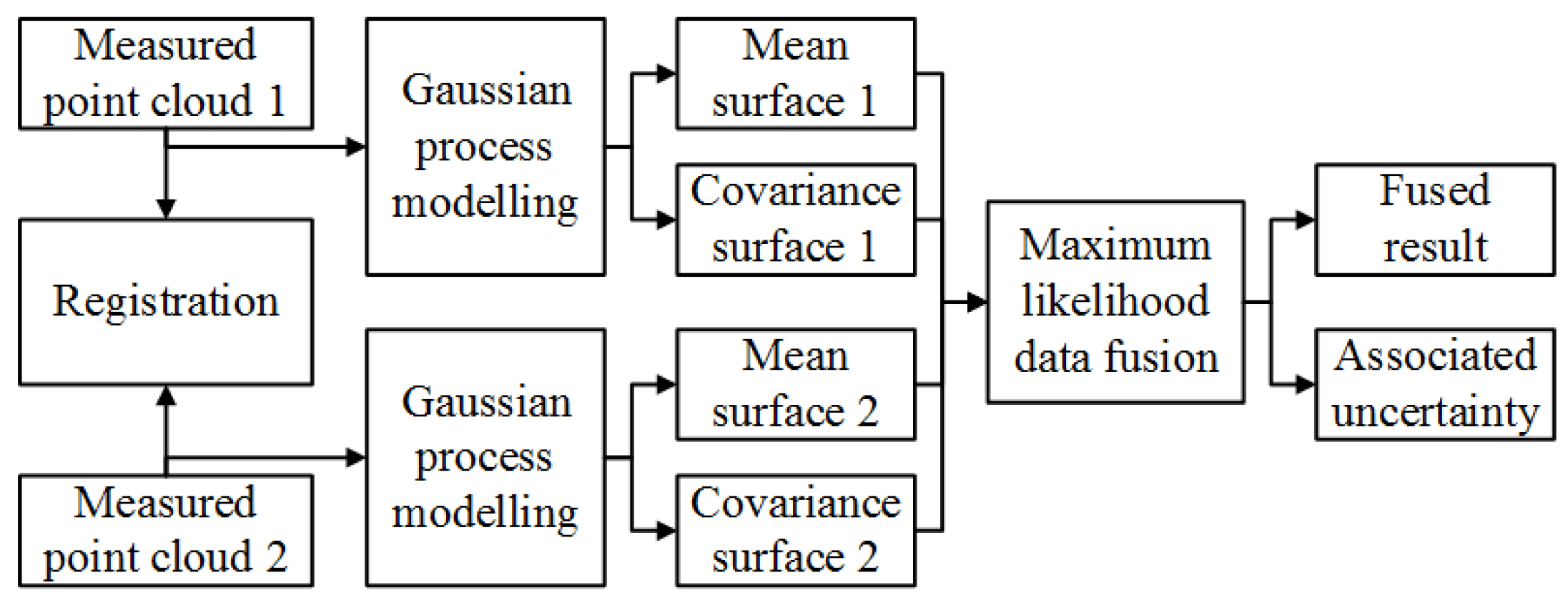
2. Gaussian Process Data Modelling and Maximum Likelihood-Based Data Fusion Method

A schematic diagram of the proposed Gaussian process data modelling and maximum likelihood data fusion method is shown in Figure 1. It starts with the registration of two datasets to a common coordinate system. The measured data of the CMM is presented in a point cloud format while the global coordinate information for different sensors is determined in advance in the calibration process, by using a standard calibration ball. However, Shen et al. [17] reported that there still existed small residual error regarding the sensor’s related position at the micrometre level. To further improve the overall accuracy of the measurement process, the datasets are first registered to a single coordinate system with the ICP (Iterative Closest Point) algorithm [18]. This aims to perform fine registration since the coordinate information of the two datasets is calibrated before the measurement so coarse registration is undertaken. After registration, the datasets are aligned in a common coordinate system. The measurement datasets are then modelled using the Gaussian process, and the mean surfaces and the covariance surfaces of the measurements are obtained at the same locations. Hence, the mean surfaces and the covariance surface are fused together using the maximum likelihood data fusion algorithm. In the end, the best estimated underlying surface and its associated measurement uncertainty are determined. In this method, Gaussian process modelling is used to determine the underlying surface and its measurement uncertainty for each measurement from different sensors. With the measurement data and the uncertainty information, the maximum likelihood data fusion is used to determine the best estimated result in a statistical manner. The details of the proposed generalized data fusion method are explained in the following sections.

2.1. Gaussian Process Data Modelling

In the present study, the measured point clouds are modelled using the Gaussian process. A Gaussian process is a generalization of the Gaussian probability distribution [13]. There is always noise in the measurement process and the noise is supposed to follow the Gaussian distribution. In the CMM measurement process, the measurement result can be determined by Equation (1).

$$z=f\left(x\right)+\mathsf{\epsilon },$$

(1)

where $z$ is the measurement result, $f\left(x\right)$ is the true value, $x$ is the input vector which represents the measured location, and $\mathsf{\epsilon }$ is the measurement error which is of Gaussian distribution with zero mean and variance ${\mathsf{\sigma }}_n^2$, hence,

$$\mathsf{\epsilon }\sim {\rm N}\left(0,{\sigma }_n^2\right),$$

(2)

Since the true value $f\left(x\right)$ is unknown and hereby the aim of using the Gaussian process is to estimate the $f\left(x\right)$ and the associated uncertainty, the Gaussian process can be defined by the mean function and covariance function:

$$f\left(x\right)\sim \mathrm{GP}\left(m\left(x\right),k\left(x,x^{\prime }\right)\right),$$

(3)

where $m\left(x\right)$ is the mean function at location $x$ and $k\left(x,x^{\prime }\right)$ is the covariance function evaluated at $x$ and $x^{\prime }$, which can be determined by:

$$\begin{gathered} m\left(x\right)=E\left[f\left(x\right)\right], \\ k\left(x,x^{\prime }\right)=E\left[\left(f\left(x\right)-m\left(x\right)\right)\left(f\left(x^{\prime }\right)-m\left(x^{\prime }\right)\right)\right], \end{gathered}$$

(4)

Equation (3) shows that $f\left(x\right)$ is fully defined by the mean function and covariance function in Gaussian process modelling. Once the model is established, any prediction ${\mathrm{f}}_{*}$ at new location $X_{*}$ can be given by the joint distribution of the measured values and the function values at the test locations:

$$\left[\begin{array}{c}z\\ {\mathrm{f}}_{*}\end{array}\right]\sim N\left(0,\left[\begin{array}{cc}K\left(X,X\right)+{\mathsf{\sigma }}_n^{2}I& K\left(X,X_{*}\right)\\ K\left(X_{*},X\right)& K\left(X_{*},X_{*}\right)\end{array}\right]\right),$$

(5)

where I is the identity matrix, $X$ is the matrix of the measured locations, $X_{*}$ is the matrix of predictive locations, and ${\mathsf{\sigma }}_n^2$ is the noise variance.

Hence, the predictive equation for Gaussian process regression is

$${\mathrm{f}}_{*}|X,z,X_{*}\sim N\left({\overline{\mathrm{f}}}_{*},\mathrm{cov}\left({\mathrm{f}}_{*}\right)\right),$$

(6)

where

$$\begin{gathered} {\overline{\mathrm{f}}}_{*}=E\left[{\mathrm{f}}_{*}|X,z,X_{*}\right]=K(X_{*},X){\left[K\left(X,X\right)+{\mathsf{\sigma }}_n^{2}I\right]}^{-1}z, \\ \mathrm{cov}\left({\mathrm{f}}_{*}\right)=K\left(X_{*},X_{*}\right)-K\left(X_{*},X\right){\left[K\left(X,X\right)+{\mathsf{\sigma }}_n^{2}I\right]}^{-1}K\left(X,X_{*}\right), \end{gathered}$$

(7)

In the present study, Gaussian process modelling is undertaken by using the Gaussian processes for machine learning (GPML) toolbox [19]. The mean function is chosen to be zero mean since the underlying surface is supposed to be unknown. Choosing zero mean surface may affect the accuracy and efficiency of Gaussian process modelling; combining Gaussian process modelling with local topological consideration [20] may be considered in future studies. The covariance function is chosen to be the most popular squared exponential function which can model smooth surface and is infinitely differentiable [13], since the measured surface in this study is continuous freeform surface. The covariance function is determined by:

$$k\left(x_i,x_j\right)={\mathsf{\sigma }}_n^2\exp \left(-\frac{{\left(x_i-x_j\right)}^2}{2l^2}\right)$$

(8)

where $l$ is the characteristic length-scale, i.e., the length over which there is no significant relationship between two z values.

Since the Gaussian process is a machine learning process, the parameters of the model are first initiated and then optimized by minimizing the negative log marginal likelihood. This is implemented in an iterative process in the GPML toolbox.

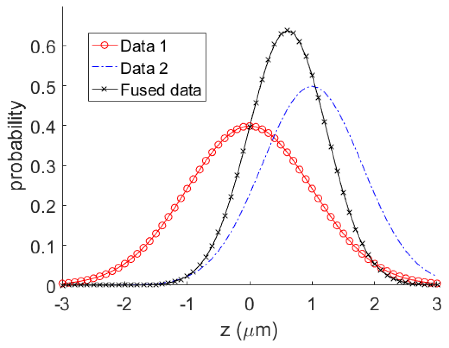
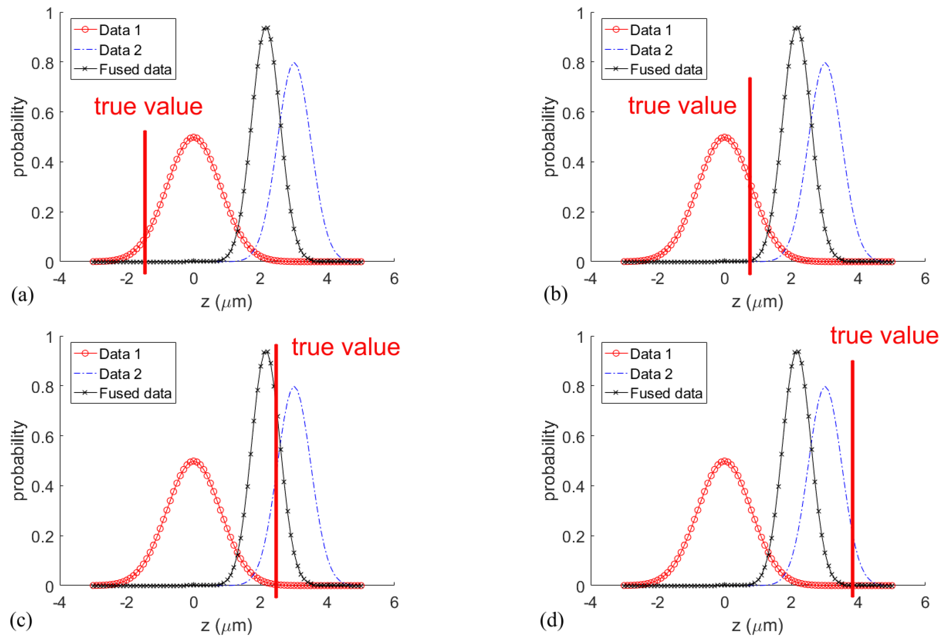
2.2. Maximum Likelihood Data Fusion

After Gaussian process modelling, the mean surface and the associated uncertainty at any position can be estimated for each measurement. For a particular multi-sensor CMM measurement which considers measurement datasets from two different sensors, the mean surfaces and the associated measurement uncertainties can be denoted as $m_1,m_2$ and $u_1,u_2$, respectively. As the measurement noise is governed by Gaussian distribution, i.e., the probability of both measurements obtaining result m can be determined by

$$\begin{gathered} p\left(m|m_1,u_1{}^2\right)=\frac{1}{u_1\sqrt{2\mathsf{\pi }}}{e}^{-\frac{{\left(m-m_1\right)}^2}{2u_1{}^2}}, \\ p\left(m|m_2,u_2{}^2\right)=\frac{1}{u_2\sqrt{2\mathsf{\pi }}}{e}^{-\frac{{\left(m-m_2\right)}^2}{2u_2{}^2}}, \end{gathered}$$

(9)

For a particular measurement at a specified position, the likelihood of both sensors observing $m$ is

$$p\left(m|m_1,u_1{}^2,m_2,u_2{}^2\right)=p\left(m|m_1,u_1{}^2\right)p\left(m|m_2,u_2{}^2\right)=\frac{1}{2\mathsf{\pi }{u}_1{u}_2}{e}^{-\left[\frac{{\left(m-m_1\right)}^2}{2u_1{}^2}+\frac{{\left(m-m_2\right)}^2}{2u_2{}^2}\right]},$$

(10)

The natural logarithm of the above function is

$$\ln \left(p\left(m|m_1,u_1{}^2,m_2,u_2{}^2\right)\right)=-\left[\frac{{\left(m-m_1\right)}^2}{2u_1{}^2}+\frac{{\left(m-m_2\right)}^2}{2u_2{}^2}\right]+C,$$

(11)

where $C=\ln \left(\frac{1}{2\mathsf{\pi }{u}_1{u}_2}\right)$.

According to the maximum likelihood principle, the best estimation for $m$ can be determined when Equation (11) is maximized, which yields

$$\widehat{m}=\arg \max \left[\ln \left(p\left(m|m_1,u_1{}^2,m_2,u_2{}^2\right)\right)\right],$$

(12)

Hence,

$$\frac{\partial \ln \left(p\left(m|m_1,u_1{}^2,m_2,u_2{}^2\right)\right)}{\partial m}=\frac{\partial \left(-\left[\frac{{\left(m-m_1\right)}^2}{2u_1{}^2}+\frac{{\left(m-m_2\right)}^2}{2u_2{}^2}\right]+C\right)}{\partial m}=0,$$

(13)

Thus,

$$\frac{2\left(\widehat{m}-m_1\right)}{2u_1{}^2}+\frac{2\left(\widehat{m}-m_2\right)}{2u_2{}^2}=0,$$

(14)

The best estimated value $\widehat{m}$ can be determined

$$\widehat{m}=\raisebox{1ex}{$\left(\frac{m_1}{u_1^2}+\frac{m_2}{u_2^2}\right)$}\!\left/ \!\raisebox{-1ex}{$\left(\frac{1}{u_1^2}+\frac{1}{u_2^2}\right)$}\right.$$

(15)

Define weights

$$w_1=\frac{1}{u_1^2}\mathrm{and}{w}_2=\frac{1}{u_2^2}$$

(16)

Equation (15) can be rewritten as

$$\widehat{m}=\frac{w_1{m}_1+w_2{m}_2}{w_1+w_2}$$

(17)

Using the uncertainty propagation principle [21], the uncertainty for $\widehat{m}$ can be determined as

$$\widehat{u}=\sqrt{{\left(\frac{w_1}{w_1+w_2}{u}_1\right)}^2+{\left(\frac{w_2}{w_1+w_2}{u}_2\right)}^2}=\sqrt{{\left(\frac{\frac{1}{u_1}}{\frac{1}{u_1^2}+\frac{1}{u_2^2}}\right)}^2+{\left(\frac{\frac{1}{u_2}}{\frac{1}{u_1^2}+\frac{1}{u_2^2}}\right)}^2}=\frac{1}{\sqrt{\left(\frac{1}{u_1^2}+\frac{1}{u_2^2}\right)}}$$

(18)

Using the weight denotation yields the uncertainty value $\widehat{u}$

$$\widehat{u}=\frac{1}{\sqrt{w_1+w_2}}$$

(19)

Equation (19) shows that the fused uncertainty has a smaller value than that from each of the original measurement data.

2.3. Data Modelling and Data Fusion Principle from the View of Dimensional Measurement Science

From a statistical point of view, the measurement dataset that has a smaller measurement uncertainty has a larger weighting in relation to the fused measurement value and vice versa. It is intuitively understood that there is a bias towards the measurement data which is more accurate. Equation (19) also shows that the fused uncertainty is smaller than any other uncertainty from the original measurement data. The fusion of two Gaussian distributions is illustrated in Figure 2. The horizontal axis denotes the measurement value at a specific position and the vertical axis denotes the probability of obtaining that measurement value. The two measurement datasets are of Gaussian distribution and are denoted as Data 1 and Data 2 in Figure 2. Data 2 is more accurate than Data 1 since Data 2 has a smaller standard deviation. The fused data has an even smaller standard deviation which illustrates that it has improved accuracy.

Due to the nature of dimensional measurement, every measurement result has associated uncertainty and the true value is never known. Moreover, there are systematic errors and random errors contained in the measurement result. The systematic error denotes the bias from the estimated mean value to the true value while the random error complies with the Gaussian distribution of the measurement result which represents the measurement uncertainty. In the procedure of maximum likelihood-based multi-sensor data fusion, the fusion algorithm takes into account both the systematic error and random error and calculates the fused result in a statistical manner. It is easy to understand that the output uncertainty is reduced in the fusion result since the fusion procedure itself can be considered as a multiple (double) measurement process which can reduce the measurement uncertainty compared to single measurement in the final result [22]. It is interesting to note that the weights for each dataset are determined by the associated uncertainties, i.e., the random errors. If a measurement has large systematic error but small random error while another measurement has small systematic error but large random error, the fused result will have a large bias to the measurement with small random error, which will introduce a large systematic error in the fused result.

This issue also exists in other fusion methods such as weighted least square fusion [23]. This is especially true for state-of-the-art technology where the measurement instruments have high repeatability with very low measurement noise. However, the systematic error is sometimes large as compared to the random error, which means that the repeatability is high but the accuracy is not ensured (may deviate from the true value) [24]. On the other hand, with advanced technology such as the precision calibration method, the systematic error of CMMs is controlled well, which can reduce the influence of this effect. The influence of the systematic error and random error on the fused result under different situations is shown in Figure 3. With two different measurement datasets Data 1 and Data 2, it is assumed that Data 2 has smaller uncertainty than Data 1, the fused result Df has smaller uncertainty than both Data 1 and Data 2, and the mean of Df has a bias towards Data 2, which is shown in Figure 3. It is interesting to note that the true value (short as Tv) of the measurement is unknown and it can be considered under the following four situations: (a) $Tv<M1<M2$; (b) $M1<Tv<M2$ (bias to M1); (c) $Tv<M1<M2$ (bias to M2); and (d) $M1<M2<Tv$, where M1 and M2 are the mean values of Data 1 and Data 2. The case shown in Figure 3c is the ideal case, which has the optimal result that the fused result has the smallest bias to the true value. The case shown in Figure 3a is the worst case in which the fused result has the largest bias to the true value.

In practice, the sensor with small measurement uncertainty usually possesses a small systematic error. This is particularly true when comparing an optical sensor with contact sensor which are widely used in multi-sensor CMMs, e.g., the laser sensor has large uncertainty and large systematic error while the touch trigger probe has small uncertainty and small systematic error. The case shown in Figure 3d is another case in which the fused result has a smaller uncertainty: it has a smaller bias than Data 1 but larger than Data 2. This is the case that should be paid much attention in multi-sensor data fusion for dimensional measurement. In general, with a sophisticated designed multi-sensor CMM, the case shown in Figure 3c is the most desired case statistically, since the true value should be among the two mean values of the different measurements and bias to the sensor with a higher accuracy in a well-calibrated situation. In fact, this situation has the highest probability in the measurement process.

In this study, the mean value and associated uncertainty for the measurement datasets are not directly given by the measurement instrument but they are modelled using the Gaussian process modelling method. Due to the existence of measurement uncertainty, the data points in the measurement result cannot represent the mean surface but are Gaussian distributed along the mean surface. The use of Gaussian process data modelling aims to model the raw data to obtain the mean surface and the associated uncertainty at every position of interest. The mean surface can be treated as the best estimated true value for the surface. With a sophisticated designed multi-sensor CMM and a well-established Gaussian process model, the mean surfaces from two different sensors should be consistent with each other with small systematic error. However, in some cases in which the accuracy requirement is stringent, the measurement error from the hardware and the modelling error from the Gaussian process method may influence the final result, especially when one of the sensors has a large systematic error.

3. Experiments and Discussion

To demonstrate the effectiveness and limitation of the proposed method, a series of simulated and real measurements with a sinusoidal surface and an f-theta lens surface was carried out. The weakness of the Gaussian process modelling was also demonstrated in a series of evaluation experiments. The real measurement experiments were conducted on a Werth VideoCheck UA multi-sensor CMM (Werth Messtechnik GmbH, Gießen, Germany) (see Figure 4) and the results were analysed and discussed. The designed and machined sinusoidal and f-theta lens freeform surface are shown in Figure 5. Two sensors were used in the measurement experiment: one is the Werth opto-electronic non-contact laser distance sensor (Werth Messtechnik GmbH, Gießen, Germany) and the other is the trigger probe Renishaw TP200 (Renishaw plc, Gloucestershire, UK) with a 1.997-mm diameter tip. The probing error of the trigger probe is ±0.65 µm while the probing error of the laser sensor is ±1.0 µm. The Maximum Permissible Measuring Error (MPE) of the CMM is (0.75 + L/300) µm. The experiment was conducted in a clean room and the environmental temperature was 20 ± 1 °C.

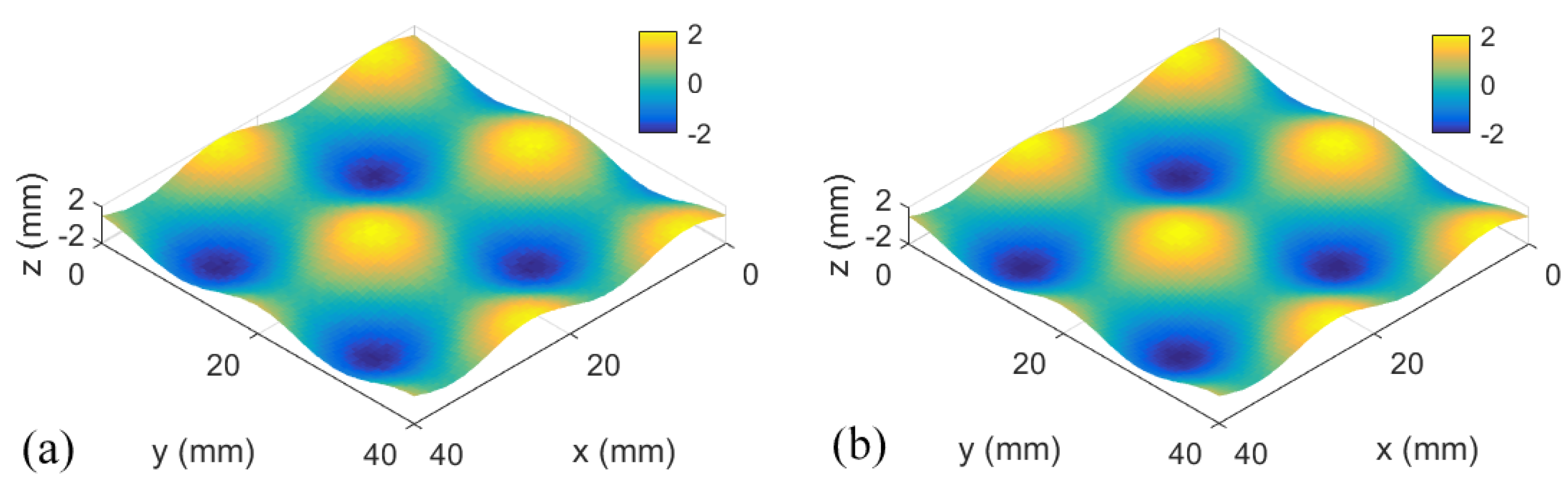
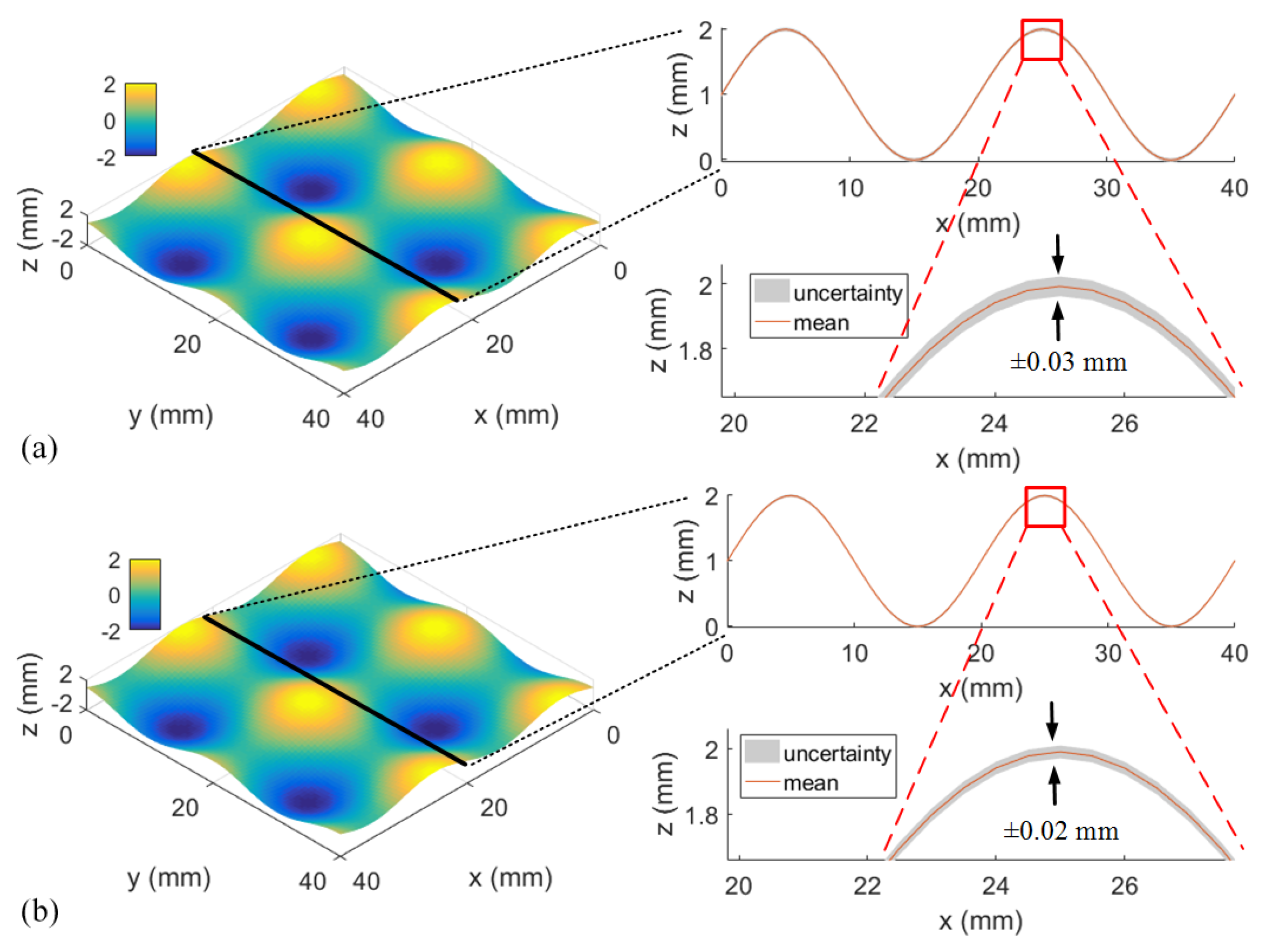
3.1. Simulated Experiments

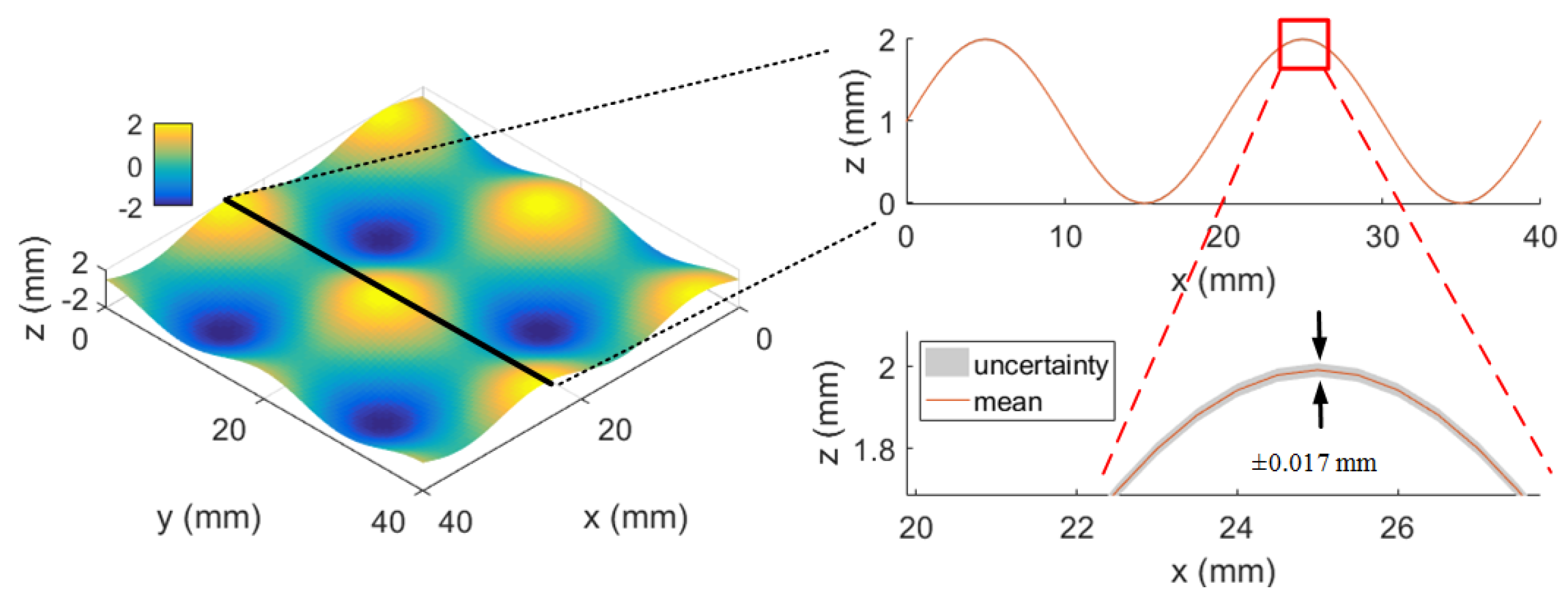
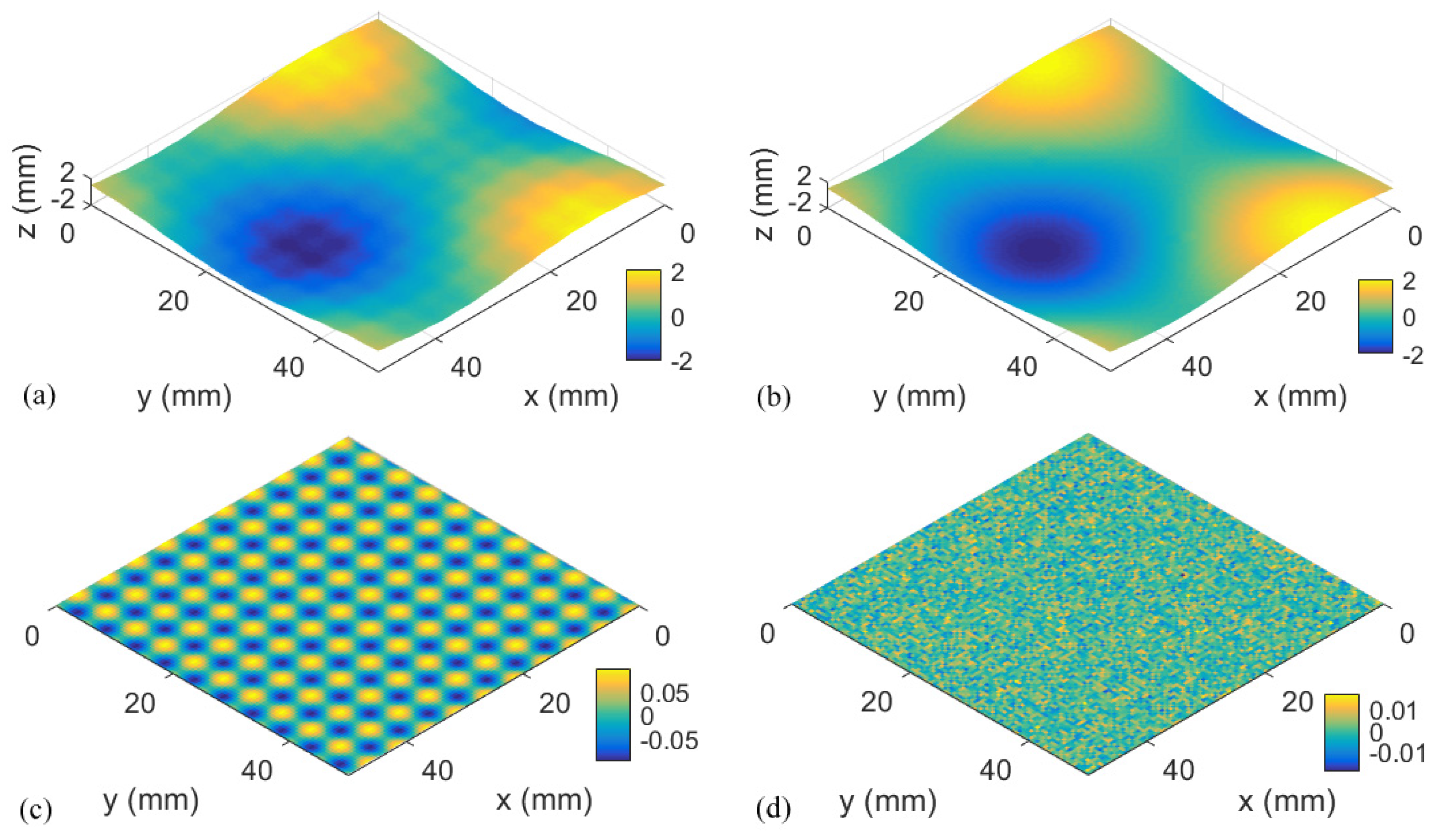
3.1.1. Sinusoidal Surface

The first experiment simulated the measurement of a sinusoidal surface with two different sensors. For each sensor, the measurement had different uncertainty values. Figure 6 shows the simulated measurement results and the measurement can be determined as:

$$z_{1,2}=\sin \left(\frac{\mathsf{\pi }}{10}x\right)+\cos \left(\frac{\mathsf{\pi }}{10}y\right)+{\mathsf{\epsilon }}_{1,2},$$

(20)

where ${\mathsf{\epsilon }}_1=30$ µm and ${\mathsf{\epsilon }}_2=20$ µm are the added normal distributed noises, which represent different measurement uncertainties.

Modelling of the two measured datasets was undertaken by the Gaussian process method. In the Gaussian process modelling, the mean function was initially chosen to be zero mean function and the covariance function was Squared Exponential function, while the likelihood function was specified to be Gaussian. The parameters of the covariance function corresponding to unit characteristic length-scale and unit signal standard deviation were firstly initiated to be zeros and the likelihood parameter was initiated to be $\ln \left(0.1\right)$, which denotes the standard deviation of the noise to be 0.1 mm. The parameters of the Gaussian process were then optimized by minimizing the negative log marginal likelihood. The results of Gaussian process modelling are shown in Figure 7. The covariance is shown in a profile view for better illustration. The root mean squared (RMS) values of the covariance surfaces are 29.8 µm and 19.8 µm, and the modelling errors are both 0.2 µm, which clearly demonstrate the effectiveness of modelling the noise for the two measurement datasets.

The fused result with maximum likelihood data fusion algorithm is shown in Figure 8. The result shows that the overall uncertainty value is reduced and the RMS value of the covariance surface is 16.5 mm, which is smaller than both of the original measurement data.

The deviations from the original measured surfaces and fused surface to the underlying surface were evaluated and the result is shown in Figure 9. Figure 9a,b shows the evenly distributed patterns along the whole surface which demonstrates the effectiveness of the modelling method and choice of zero mean surface. It is interesting to note that the edge area of the measurement results, especially the corner area, has a larger prediction error since there are insufficient measurement data in those areas.

Table 1. RMS (root mean squared) value of associated uncertainties of the original measurement datasets and fused dataset.

Evaluation Items	With Sensor 1	With Sensor 2	Fused Data
RMS of uncertainty	29.8 µm	19.8 µm	16.5 µm
RMS of deviation	3.5 µm	2.4 µm	2.2 µm

shows the RMS value of the uncertainties and the deviations for the original measurement datasets and the fused dataset. The result clearly shows that both the uncertainty and the deviation from the reference surface have improvements over the original measurement results.

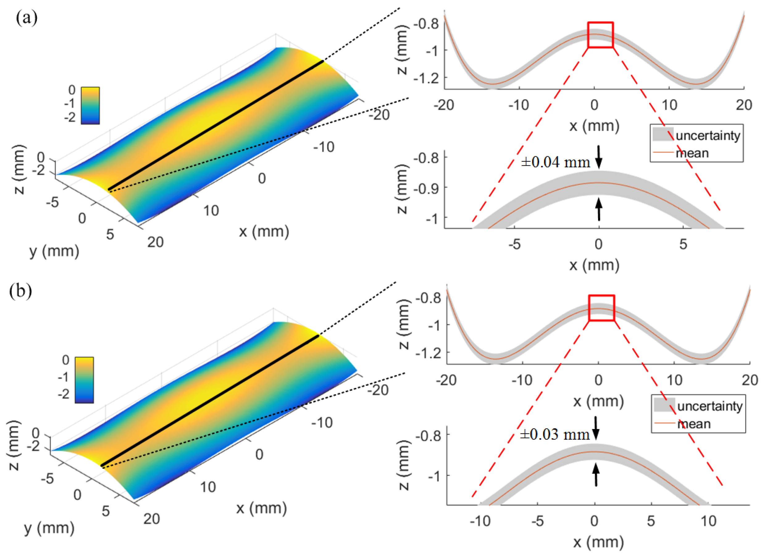
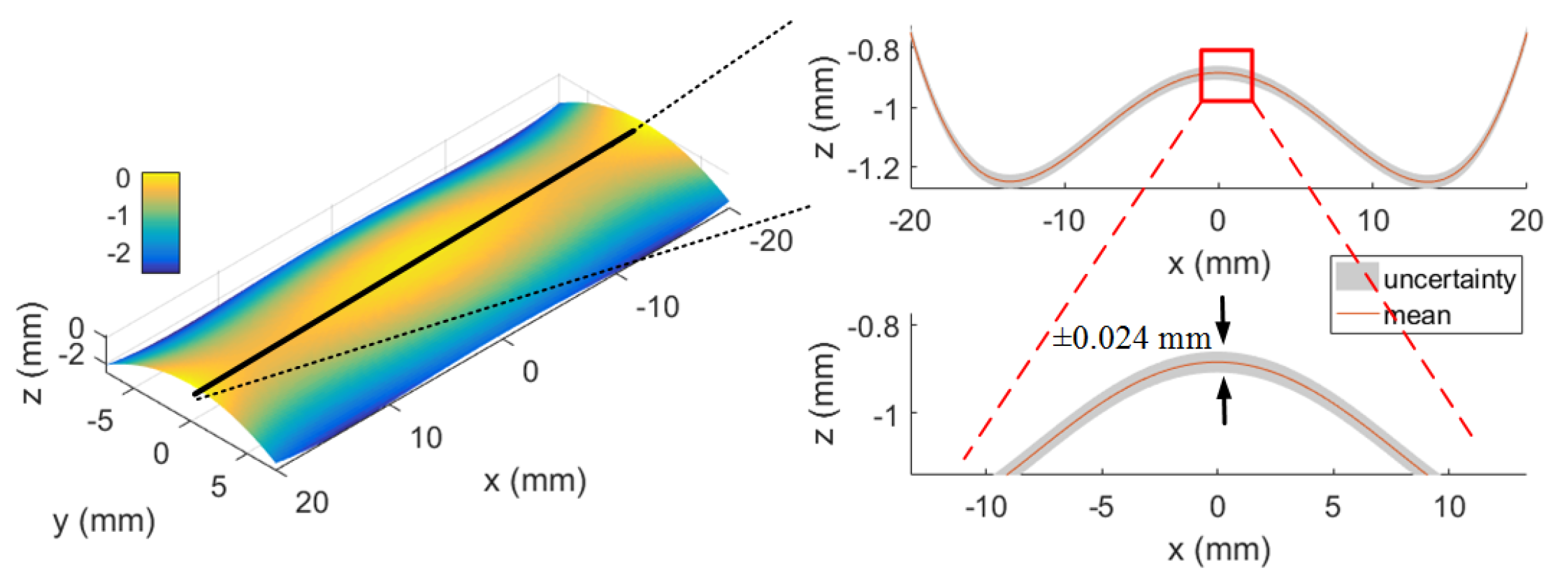
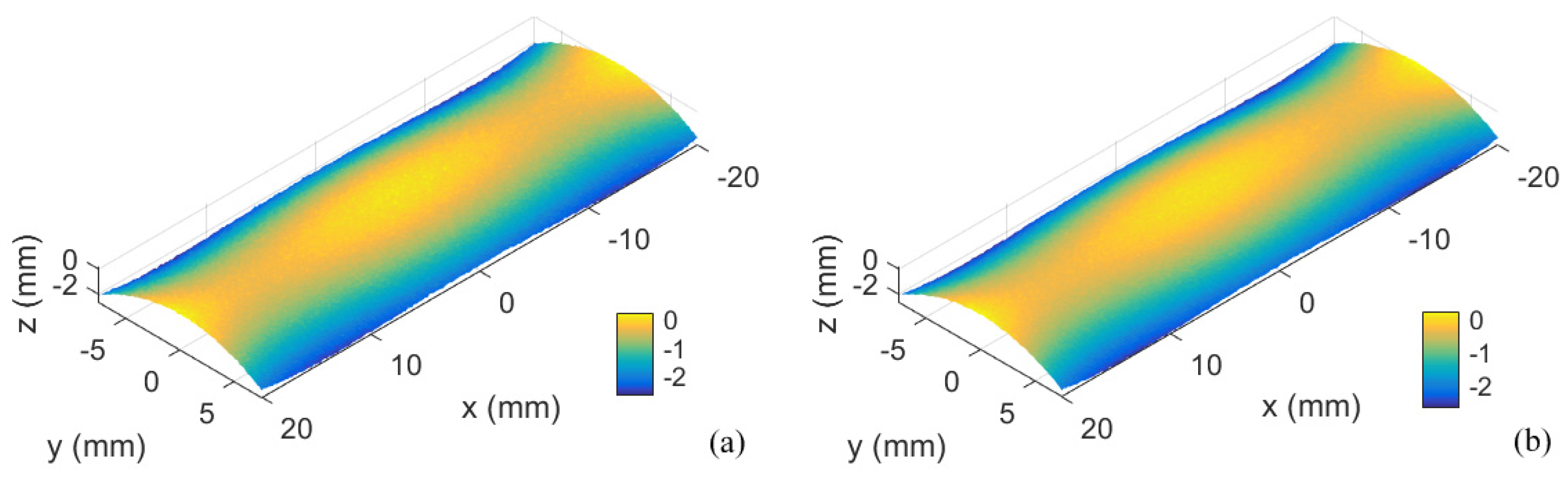
3.1.2. F-Theta Lens Surface

Another simulation experiment was conducted on an f-theta lens freeform surface to evaluate the proposed method. Compared with the sinusoidal surface, the f-theta lens surface is relatively smoother without periodical features. The measurement of the f-theta lens surface is determined by:

$$z_{1,2}=a{x}^2+b{x}^4+c{y}^2+{\mathsf{\epsilon }}_{1,2},$$

(21)

where $a=-1/250$, $b=1/92,000$ and $c=-1/25$ are the design parameters of the surface and ${\mathsf{\epsilon }}_1=40$ µm and ${\mathsf{\epsilon }}_2=30$ µm are the added normal distributed noises which represent the different measurement errors. Figure 10 shows the simulated measurement surfaces.

Figure 11 shows the results of Gaussian process modelling with the mean surface and the covariance surface determined. The RMS values of the covariance surface are 38.6 µm and 31.0 µm and the modelling error are 1.4 µm and 1.0 µm, respectively. The results show that the measurement uncertainty is estimated well using the Gaussian process. Figure 12 shows the result after maximum likelihood data fusion. The RMS value of covariance surface is 24.2 µm which is smaller than that from the original covariance surface, and this is expected from the use of the data fusion principle.

The deviations from the original surfaces and the surface after data fusion to the underlying surface are shown in Figure 13. Figure 13a,b presents the evenly distributed patterns along the whole surface which realizes the effectiveness of the modelling method and choice of zero mean surface. The RMS value of the uncertainties and deviations are shown in

Table 2. RMS (root mean squared) value of associated uncertainties of the original measurement datasets and fused dataset.

Evaluation Items	With Sensor 1	With Sensor 2	Fused Data
RMS of uncertainty	38.6 µm	31.0 µm	24.2 µm
RMS of deviation	2.3 µm	2.1 µm	1.8 µm

. Both the uncertainties and the deviations of the fusion result indicate improvement as compared with the original datasets. Similar to the one for the sinusoidal surface, the error in the edge and corner area are larger since the data in those areas are insufficient.

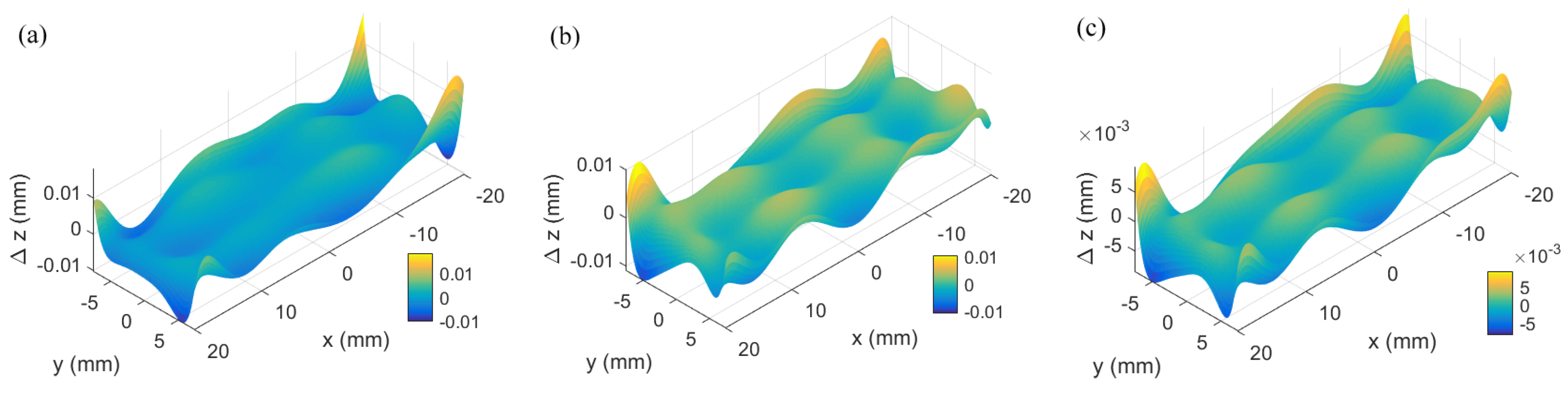
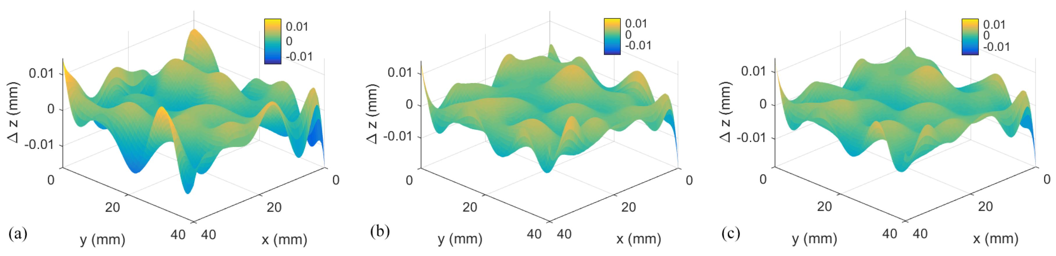
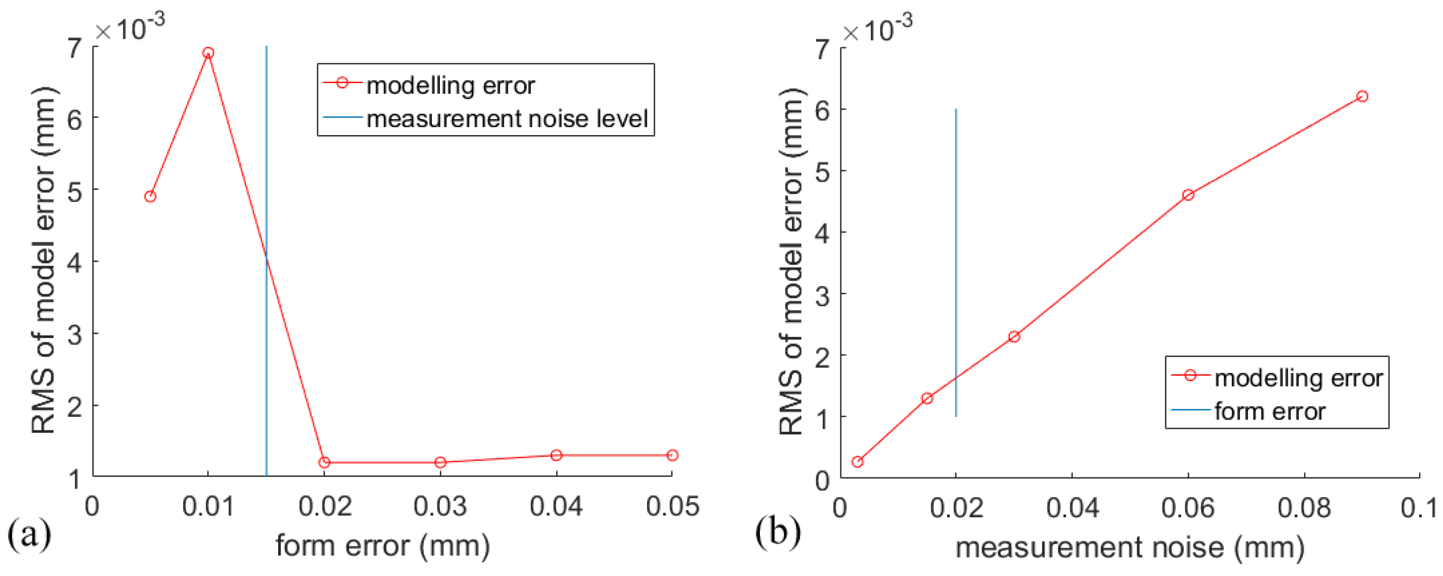
3.2. Model Error Analysis for Gaussian Process Modelling

In the previous simulation experiments, the measurement noises were modelled well using the Gaussian process modelling method. However, in real-life situations, machined surfaces are not perfect and may contain defects and form error due to machining error which may affect the modelling accuracy of the Gaussian process. In this section, a series of simulation experiments was conducted to verify the effectiveness and limitations of Gaussian process modelling by adding the form error to the simulated surface. That is to say, the simulated surface has a base form, form error and measurement noises, as shown in Figure 14. The base form is a sinusoidal surface with lateral pitch of 50 mm, the peak-to-valley (PV) value is 4 mm and the surface is denoted by $S_b$. The machining error denoted by $S_e$ is simulated to be a sinusoidal deviation from the base form with a higher spacial frequency together with a pitch of 5 mm and smaller peak-to-valley height (PV) value of 0.1 mm, and the PV value is varied in a series of experiments in order to validate the model. The combination of the base form and the form error determines the actual form ($S_c$) of the surface as shown in Equation (22):

$$S_c=S_b+S_e,$$

(22)

For the measurement noise $N$, it is simulated to be Gaussian distributed noise with zero mean and 0.005 mm standard deviation, the expended deviation is 0.015 mm (k = 3), and this amplitude is also varied to test the performance of the model. The simulated measurement result of the surface is denoted as $S_m$:

$$S_m=S_b+S_e+N,$$

(23)

The experiment was conducted as follows. The amplitude of the base form was fixed as ±2 mm and the standard deviation of the measurement noise was fixed as 0.005 mm. The expanded deviation of the measurement noise level (k = 3) was 0.015 mm. The amplitudes of the form errors in the experiments were simulated to be ±0.005 mm, ±0.01 mm, ±0.02 mm, ±0.03 mm, ±0.04 mm and ±0.05 mm. The simulated measurement result of the surface $S_m$ was then modelled by using the Gaussian process modelling method and the mean surface $S_{\mathrm{mean}}$ and the covariance surface $S_{\mathrm{cov}}$ were calculated. The objective function $O_E$ of the performance of the Gaussian process model was determined by the RMS of the deviation from the mean surface $S_{\mathrm{mean}}$ to $S_c$:

$$O_E=\mathrm{RMS}(S_{\mathrm{mean}}-S_c),$$

(24)

The result of the experiment is shown in Figure 15a. The result shows that when the form error is smaller than the measurement noise, the error of the model is large, while when the form error is larger than the measurement noise, the error of the model is small. This result demonstrates that when the form error is smaller than or similar to the measurement noise, the model has the limitation of being unable to distinguish the form error and measurement noise which leads to a large modelling error that treats both the form error and the measurement noise as the measurement noise. This leads to an overestimation of the overall uncertainty of the measurement.

Another experiment was conducted to fix the base form and the form error, and change the amplitude of the measurement noise. The amplitude of the base form was also fixed as ±2 mm as in the previous experiment while the form error was fixed as ±0.02 mm. The standard deviations of the measurement noise were simulated to be 0.001 mm, 0.005 mm, 0.01 mm, 0.02 mm and 0.03 mm. The method of evaluation of the performance of the model is similar to previous experiments and the result is shown in Figure 15b. The expanded deviation values of the measurement noise are used in the figure. The result shows that the model error increases when the measurement noise increases in a linear relationship. When the measurement noise is larger than the form error, the modelled error may also be affected by the form error but this is not clearly shown in the result since it may be covered by the effect of the large measurement noise.

In general, the experiment results show that the accuracy of the model of Gaussian process modelling is not only affected by the measurement noise but also by the form error of the measured surface, especially when the amplitude of the form error is smaller than that of the measurement noise. Considering that the model error affected by the measurement noise is in the confidence region of the uncertainty modelled by the Gaussian process which is acceptable in the result, the model error affected by the form error is not the same case since it may cause the mean surface to have a bias to the true value which is outside the confidence region of the modelling. This is one of the limitations of Gaussian process data modelling in that it affects the accuracy of the proposed method.

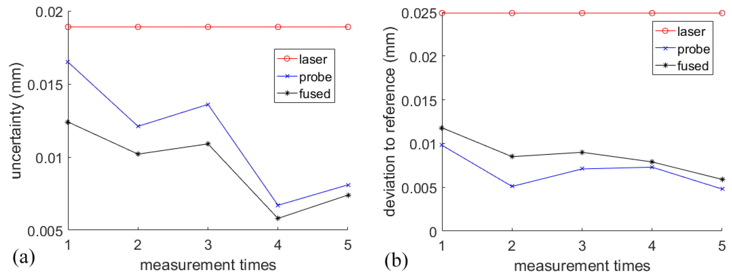
3.3. Evaluation of the Performance of Measurement Uncertainty Modelling Using the Gaussian Process

To evaluate the performance of the Gaussian process model for modelling the measurement uncertainty for a multi-sensor CMM, a repeated measurement experiment using a touch trigger probe was conducted and compared with the specification of the sensor and the result of using Gaussian process modelling. A workpiece was designed as shown in Figure 16 and eight points (marked A–H) were measured 50 times with a purposely-designed DMIS (Dimensional Measuring Interface Specification) programming language [25]. The eight points were chosen to be on a flat surface and curved surface with different tilting angles. The results show good agreement with similar distribution and Figure 17 shows one of the measurement results in a histogram and fitted Gaussian distribution. The standard deviation of the fitted Gaussian distribution is about 0.7 µm, which is at the same level of the specification of the tough trigger probe (0.65 µm).

The freeform surface shown in Figure 5a was measured using the tough trigger probe with a dense measurement (0.5 mm pitch). The measured data were modelled using Gaussian process modelling and the mean surface and the associated uncertainty are shown in Figure 18. The RMS of the uncertainty is 0.74 µm which is slightly larger than the specification of the probe and the experimental standard deviation value. The result demonstrates the effectiveness of the Gaussian process method to model measurement uncertainty. It should be noted that the uncertainties in the edge and corner areas are large due to the lack of data points in those areas and the measurement uncertainties are different with different measurement density, with less measurement points or larger sampling pitch, so it is clear that the measurement uncertainty is larger due to the reduction of measurement data.

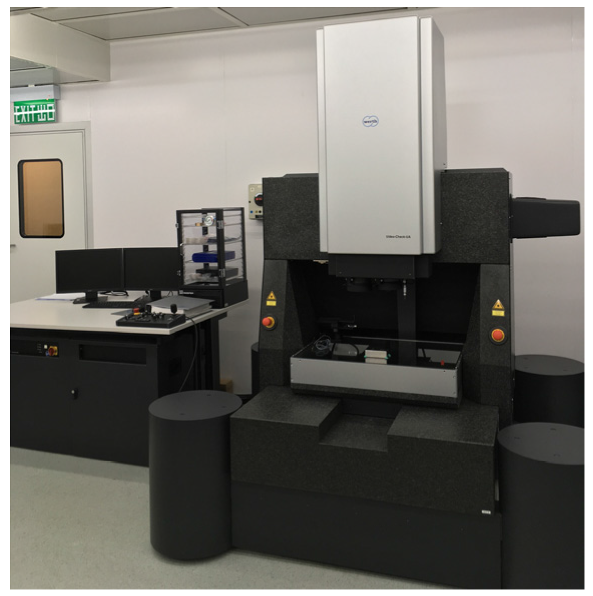
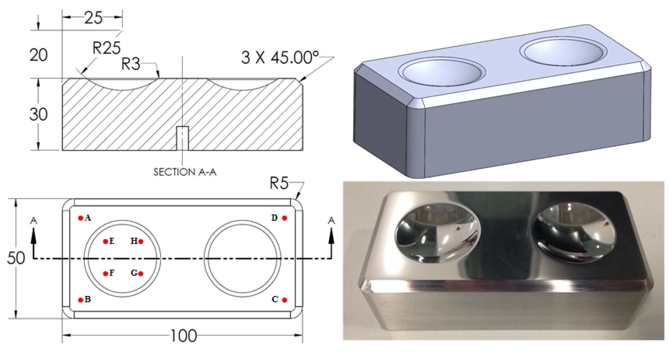
3.4. Measurement Experiment Using a Multi-Sensor CMM

The two workpieces with sinusoidal and f-theta lens surface surfaces shown in Figure 5 were measured with the Werth multi-sensor CMM with a laser sensor and touch trigger probe to demonstrate the effectiveness of the proposed data modelling and data fusion method. Generally, the laser sensor derives its strength from its non-contact measurement nature but has larger measurement uncertainty while the tough trigger probe has higher measurement accuracy with smaller uncertainty. The measurement with the laser sensor was designed to be dense and the measurement with the touch trigger probe was designed to have less sampling points.

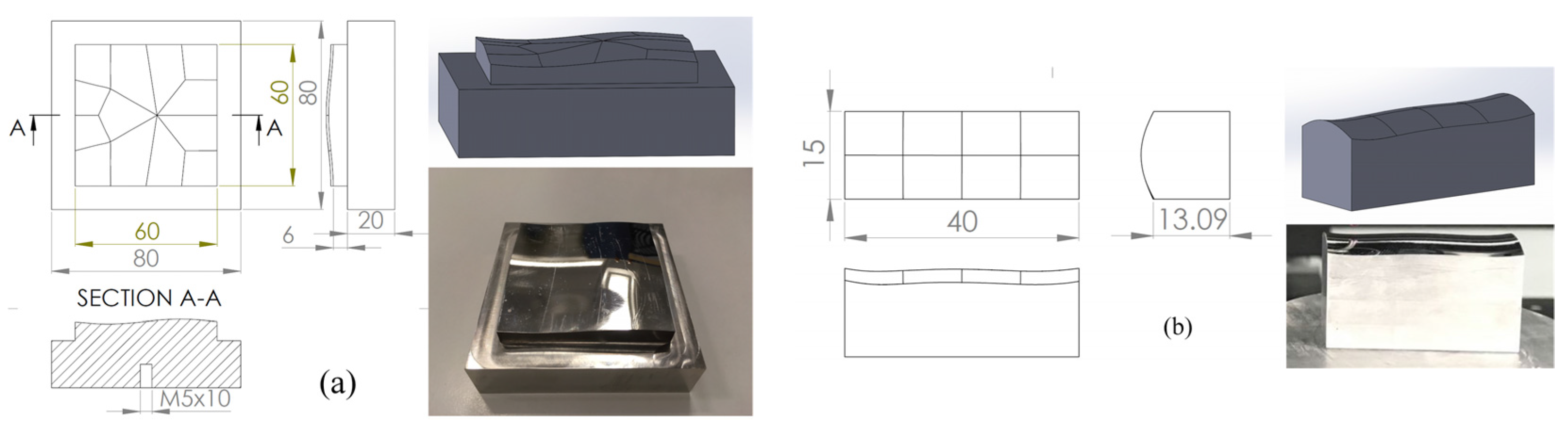
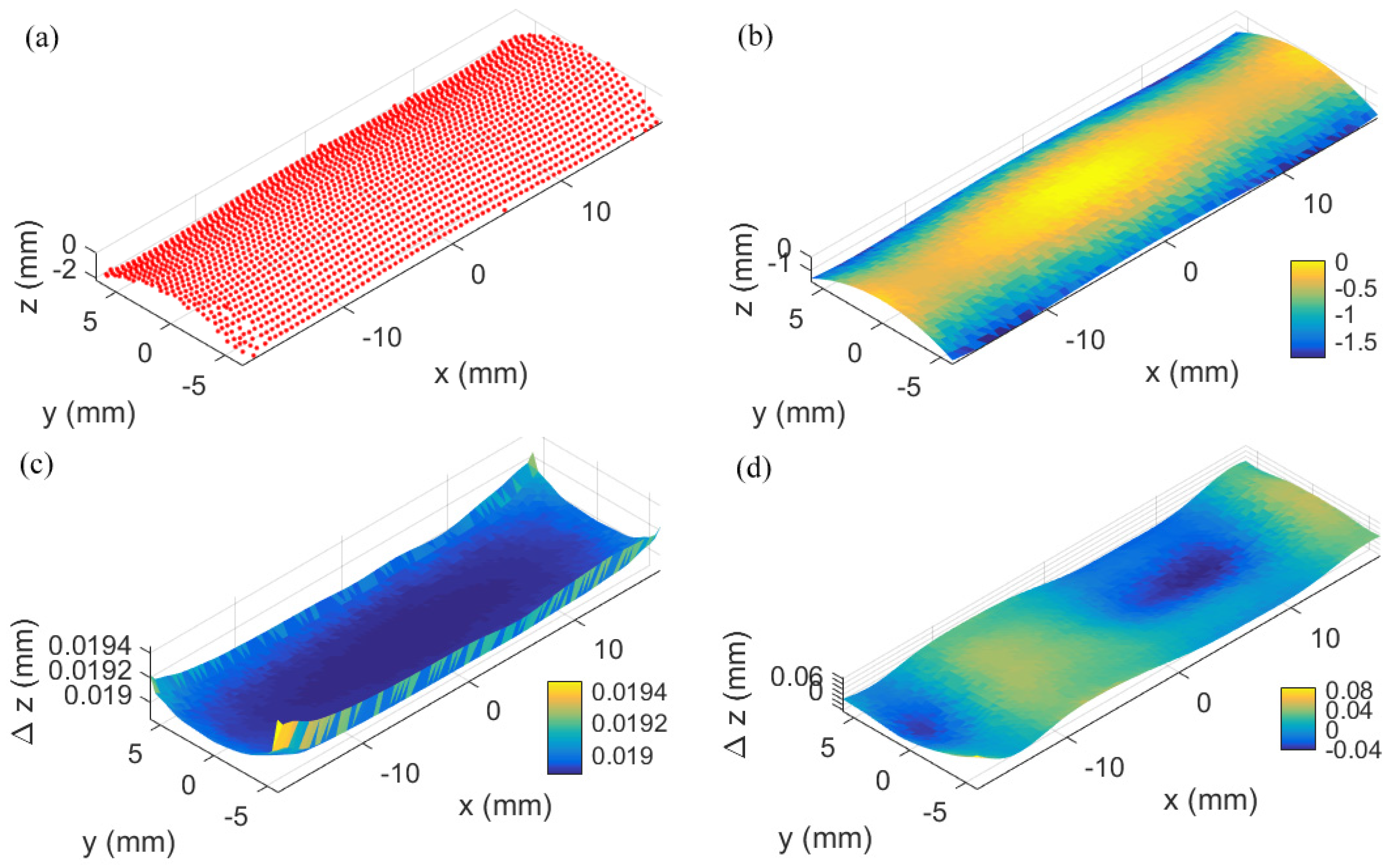
3.4.1. Measurement of a Sinusoidal Surface

The experiemnt was designed as follows. First, the sinusodial surface was measured using the touch trigger probe with a density of 0.5 mm and the measurement result was treated as the reference data since it had high density and high accuracy. Then the surface was measured using a laser sensor with a density of 1 mm pitch and this measurement result was determined as the first dataset. The measured data were then modelled using the Gaussian process and the results are shown in Figure 19. Figure 19a illustrates the raw data from the laser sensor, Figure 19b,c show the mean surface and the associated uncertainty of the Gaussian process while Figure 19d shows the deviation from the mean surface to the reference surface. The RMS of the uncertainty is 18.3 µm and the RMS of the deviation is 38.3 µm. The large measurement uncertainty may be caused by the unstable measurement by the optical sensor. It should be noted that the prediction grid for the Gaussian process has 1-mm pitch in the area where $x\in \left[-30,30\right]$ mm and $y\in \left[-30,30\right]$ mm.

A subset of 50 randomly sampled measurement points from the dense measurement data of the touch trigger probe was selected as the second dataset. The raw data and the result after the Gaussian process for the second dataset are shown in Figure 20. Figure 20a shows the raw measurement data, Figure 20b shows the mean surface, Figure 20c shows the associated uncertainty, and Figure 20d shows the deviation of the mean surface from the reference surface. Note that the grid of the prediction for the Gaussian process is the same as that for the laser sensor. The RMS of the measurement uncertainty is 15.7 µm and the RMS of the deviation map is 13.2 µm. The large measurement uncertainty is due to the small number of sampling points.

The fused result of the dataset from the laser sensor and trigger probe is shown in Figure 21. Figure 21a shows the fused mean surface, Figure 21b shows the associated uncertainty and Figure 21c shows the deviation from the fused mean surface to the reference data. The RMS of the uncertainty is 8.0 µm and the RMS of the deviation map is 8.4 µm, both showing improvements compared to the original measurement datasets.

Five different datasets for the touch trigger probe from different sampling positions were obtained and underwent the above procedure and the results are shown in Figure 22. The measurement data of the laser sensor were the same. Figure 22a shows the results of the RMS of the measurement uncertainties and Figure 22b shows the result of the RMS of the deviations. Both results show a consistent improvement of the measurement uncertainty and deviation from the reference data for the repeated measurement. The result demonstrates the effectiveness of the proposed data modelling and data fusion method. The high repeatability of the improvement of the data fusion may result from the well-established sensor configuration and high performance of data modelling which fit the situation shown in Figure 3c.

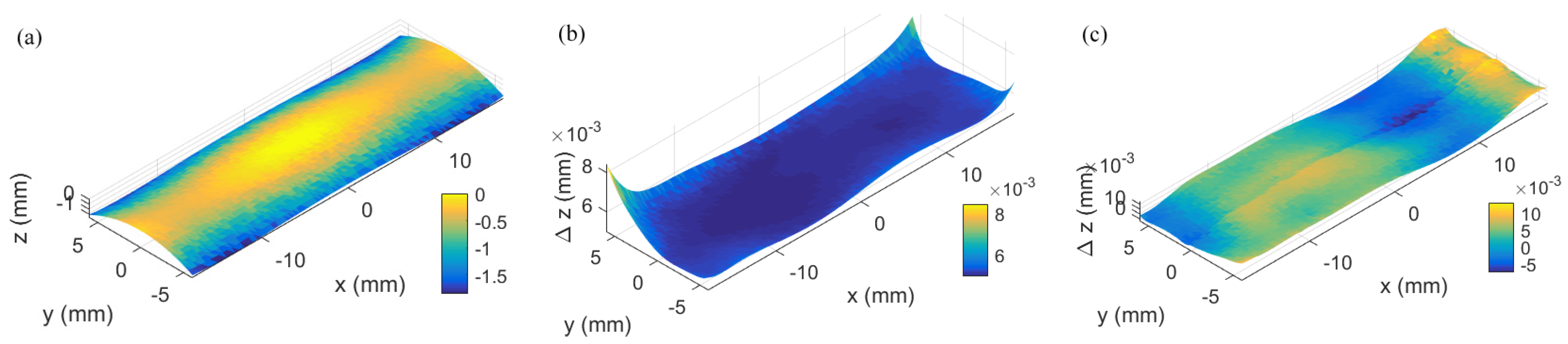
3.4.2. Measurement of an f-Theta Lens Surface

The f-theta lens freeform surface was measured in the present study. Instead of showing the improvement of the final result, this experimental result shows that when one measurement has a large systematic error, the performance of the final result will be affected. Similar to the previous experiment, the surface was measured using a touch trigger probe with a dense measurement of 0.5-mm pitch and the result was determined as the reference data. In this experiment, there existed a large systematic error in the measurement of the laser sensor which may have been caused by the outliers in the measurement result, as shown in Figure 23. It is noted that the outliers were removed in the data processing with a statistical analysis method [26]. However, there was still residual error in the dataset which may affect the final result. The outliers may be caused by the characteristics of the measured surface such as specular reflection of the reflectance light [27] which is considered to influence the optical sensor.

After the outliers were removed, the raw data were processed with Gaussian process modelling and the mean surface was obtained together with the associated uncertainty. The deviation of the mean surface to the reference surface was also determined as shown in Figure 24. The RMS of the uncertainty was 18.9 µm and the RMS of the deviation map was 24.9 µm. The result shows a larger uncertainty and even larger deviation than the previous measurement experiment which may introduce a larger systematic error for this measurement.

A subset of 50 points of the measurement data from the touch trigger probe was used as the second dataset for the measurement. The data were modelled using the Gaussian process and the mean surface and the associated uncertainty were determined. The deviation from the mean surface to the reference surface was also determined as shown in Figure 25. The RMS of the uncertainty was 5.7 µm while the RMS of the deviation map was 2.9 µm.

The fused results of the two datasets are shown in Figure 26. The RMS of fused uncertainty was 5.2 µm while the RMS of the deviation map was 4.8 µm. It is found that the fused uncertainty was improved and smaller than the original two datasets. However, the deviation is larger than the one only considering the touch trigger probe. Another five measurement results were obtained at different sampling locations and the results are shown in Figure 27. All the results show that the uncertainty was improved while the deviations were worse. This is due to the fact that the measurement data from the laser sensor have large bias from the true value which affects the final fused result. This experiment demonstrated the case similar to the situation as discussed in Figure 3d, where the true value is larger than the mean values of both original measurements. This is the limitation of the data fusion method in that when one of the sensors has large systematic error, the fused result will be poorer than when only considering the data from another sensor. Future work will be focused on the quantitative analysis of the influence of the systematic error on the fusion result. Practically, more attention should be paid to correcting the systematic error, especially that which is caused by the optical sensors such as the laser sensor. Another approach to this issue when considering the systematic error is generating adaptive weighting using a Bayesian framework [28]. In this situation, the fault-inducing systematic error may be detected and the weighting for those points can be adjusted accordingly.

4. Conclusions

Coordinate measuring machines (CMMs) equipped with multiple sensors are becoming popular in the high-end precision metrology market since their measurement ability can be enhanced by combining the datasets measured by different sensors. Development of a data modelling method for datasets measured by different sensors and an appropriate data fusion method are the key issues for measurement with multi-sensor CMMs to further enhance the measurement performance. This paper presents a data modelling and data fusion method for multi-sensor CMMs which is based on Gaussian process modelling and the Bayesian inference-based maximum likelihood principle. The raw data from different sensors are firstly modelled by the Gaussian process to obtain the mean surface and covariance surface which represent the underlying surface and the measurement uncertainty, as well as the prediction for the data at unsampled positions. The mean surface and covariance surface are then fused together using the maximum likelihood principle so as to obtain the best estimated surface and the associated uncertainty. Simulation and real experiments show that both the measurement uncertainty and prediction error at unsampled positions have improvement over single-sensor measurement. Special attention should be paid to the important aspect of avoiding or reducing the systematic error from each sensor so that the performance of the fusion algorithm can be achieved. The proposed method is a generic data modelling and data fusion method which can be implemented into various kinds of multi-sensor CMMs with different sensors. The limitation of the proposed method is that the performance is affected by the systematic error. Future work will be focused on the identification of systematic error and setting different weights according to the accuracy of the datasets regarding the systematic error and random error.

References

1. Fang, F.Z.; Zhang, X.D.; Weckenmann, A.; Zhang, G.X.; Evans, C. Manufacturing and measurement of freeform optics. CIRP Ann. Manuf. Technol. 2013, 62, 823–846. [Google Scholar] [CrossRef]
2. Hocken, R.J.; Pereira, P.H. Coordinate Measuring Machines and Systems; CRC Press: Boca Raton, FL, USA, 2016. [Google Scholar]
3. Savio, E.; De Chiffre, L.; Schmitt, R. Metrology of freeform shaped parts. CIRP Ann. Manuf. Technol. 2007, 56, 810–835. [Google Scholar] [CrossRef]
4. Weckenmann, A.; Jiang, X.; Sommer, K.D.; Neuschaefer-Rube, U.; Seewig, J.; Shaw, L.; Estler, T. Multisensor data fusion in dimensional metrology. CIRP Ann. Manuf. Technol. 2009, 58, 701–721. [Google Scholar] [CrossRef]
5. Carl Zeiss Industrial Metrology. User Manual for ZEISS O-INSPECT. Available online: http://www.zeiss.com/ (accessed on 24 July 2016).
6. Werth Messtechnik GmbH. User Manual for Werth VideoCheck UA. Available online: http://www.werth.de/ (accessed on 24 July 2016).
7. Schwenke, H.; Wäldele, F.; Weiskirch, C.; Kunzmann, H. Opto-tactile Sensor for 2D and 3D Measurement of Small Structures on Coordinate Measuring Machines. CIRP Ann. Manuf. Technol. 2001, 50, 361–364. [Google Scholar] [CrossRef]
8. Hexagon, A.B. Optiv Classic. Available online: http://hexagonmi.com/ (accessed on 24 July 2016).
9. Nikon Metrology NV. LK V-GP High accuracy gantry CMM. Available online: http://www.nikonmetrology.com/ (accessed on 24 July 2016).
10. Galetto, M.; Mastrogiacomo, L.; Maisano, D.; Franceschini, F. Cooperative fusion of distributed multi-sensor LVM (Large Volume Metrology) systems. CIRP Ann. Manuf. Technol. 2015, 64, 483–486. [Google Scholar] [CrossRef]
11. Colosimo, B.M.; Pacella, M.; Senin, N. Multisensor data fusion via Gaussian process models for dimensional and geometric verification. Precis. Eng. 2015, 40, 199–213. [Google Scholar] [CrossRef] [Green Version]
12. Qian, P.Z.; Wu, C.J. Bayesian hierarchical modeling for integrating low-accuracy and high-accuracy experiments. Technometrics 2008, 50, 192–204. [Google Scholar] [CrossRef]
13. Williams, C.K.; Rasmussen, C.E. Gaussian Processes for Machine Learning; MIT Press: Cambridge, MA, USA, 2006; Volume 2, p. 4. [Google Scholar]
14. Xia, H.; Ding, Y.; Wang, J. Gaussian process method for form error assessment using coordinate measurements. IIE Trans. 2008, 40, 931–946. [Google Scholar]
15. Yin, Y.H.; Ren, M.J.; Sun, L.J.; Kong, L.B. Gaussian process based multi-scale modelling for precision measurement of complex surfaces. CIRP Ann. Manuf. Technol. 2016, 65, 487–490. [Google Scholar] [CrossRef]
16. Xia, H.; Ding, Y.; Mallick, B.K. Bayesian hierarchical model for combining misaligned two-resolution metrology data. IIE Trans. 2011, 43, 242–258. [Google Scholar] [CrossRef]
17. Shen, T.S.; Menq, C.H. Automatic camera calibration for a multiple-sensor integrated coordinate measurement system. IEEE Trans. Robot. Autom. 2001, 17, 502–507. [Google Scholar] [CrossRef]
18. Besl, P.J.; McKay, N.D. A method for registration of 3-D shapes. IEEE Trans. Pattern Anal. Mach. Intell. 1992, 14, 239–256. [Google Scholar] [CrossRef]
19. Rasmussen, C.E.; Nickisch, H. Gaussian processes for machine learning (GPML) toolbox. J. Mach. Learn. Res. 2010, 11, 3011–3015. [Google Scholar]
20. Bukkapatnam, S.T.S.; Cheng, C. Forecasting the evolution of nonlinear and nonstationary systems using recurrence-based local Gaussian process models. Phys. Rev. E 2010, 82. [Google Scholar] [CrossRef] [PubMed]
21. The Joint Committee for Guides in Metrology (JCGM). Evaluation of Measurement Data—Guide to the Expression of Uncertainty in Measurement (GUM); JCGM: Sevres, France, 2008. [Google Scholar]
22. Taylor, J. An Introduction to Error Analysis, the Study of Uncertainties in Physical Measurements; University Science Books: Sausalito, CA, USA, 1997; Volume 1. [Google Scholar]
23. Wang, J.; Leach, R.K.; Jiang, X. Review of the mathematical foundations of data fusion techniques in surface metrology. Surf. Topogr. Metrol. Prop. 2015, 3. [Google Scholar] [CrossRef]
24. Liu, M.; Cheung, C.F.; Ren, M.; Cheng, C.-H. Estimation of measurement uncertainty caused by surface gradient for a white light interferometer. Appl. Opt. 2015, 54, 8670–8677. [Google Scholar] [CrossRef] [PubMed]
25. Werth Messtechnik GmbH. User Manual—DMIS Programming; Werth Messtechnik GmbH: Gießen, Germany, 2011. [Google Scholar]
26. Rusu, R.B.; Cousins, S. 3D is here: Point Cloud Library (PCL). In Proceedings of the 2011 IEEE International Conference on Robotics and Automation (ICRA), Shanghai, China, 9–13 May 2011; pp. 1–4.
27. Ryu, Y.; Cho, H. New optical sensing system for obtaining the three-dimensional shape of specular objects. Opt. Eng. 1996, 35, 1483–1495. [Google Scholar] [CrossRef]
28. Wang, Z.; Bukkapatnam, S.T.; Kumara, S.R.; Kong, Z.; Katz, Z. Change detection in precision manufacturing processes under transient conditions. CIRP Ann. Manuf. Technol. 2014, 63, 449–452. [Google Scholar] [CrossRef]
Figure 1. Framework of the Gaussian process and maximum likelihood-based data fusion method.
Applsci 06 00409 g001
Figure 2. Fusion of two Gaussian distributions.
Applsci 06 00409 g002
Figure 3. Influence of systematic error, random error and the true value for the fused result: (a) measurement with large systematic error but small random error, fused with measurement with small systematic error but large random error, T v < M 1 < M 2 ; (b) measurement with large systematic error but small random error, fused with measurement with small systematic error and large random error, M 1 < T v < M 2 (bias to M1); (c) measurement with small systematic error and small random error, fused with measurement with large systematic error and large random error, T v < M 1 < M 2 (bias to M2); and (d) measurement with small systematic error and small random error, fused with measurement with large systematic error and large random error, M 1 < M 2 < T v .
Applsci 06 00409 g003
Figure 4. Werth VideoCheck UA multi-sensor CMM (coordinate measuring machine) used for the experiments.
Applsci 06 00409 g004
Figure 5. The designed and machined workpieces: (a) sinusoidal workpiece; and (b) f-theta lens workpiece (unit in mm).
Applsci 06 00409 g005
Figure 6. Simulated measurement results of the designed sinusoidal surface: (a) with 30 µm measurement noise; and (b) with 20 µm measurement noise.
Applsci 06 00409 g006
Figure 7. Gaussian process modelling results of the two simulated measured datasets: (a) with 30 µm measurement noise; and (b) with 20 µm measurement noise.
Applsci 06 00409 g007
Figure 8. Fused result with the maximum likelihood data fusion method.
Applsci 06 00409 g008
Figure 9. Deviations from the underlying surface from the results of: (a) Sensor 1; (b) Sensor 2; and (c) fused data.
Applsci 06 00409 g009
Figure 10. Simulated measurement results of the designed f-theta lens surface: (a) with 40 µm measurement noise; and (b) with 30 µm measurement noise.
Applsci 06 00409 g010
Figure 11. Gaussian process modelling results of the two simulated measured datasets: (a) with 40 µm measurement noise; and (b) with 30 µm measurement noise.
Applsci 06 00409 g011
Figure 12. Fused result with the maximum likelihood data fusion method.
Applsci 06 00409 g012
Figure 13. Deviation from the underlying surface from the results of: (a) Sensor 1; (b) Sensor 2; and (c) fused data.
Applsci 06 00409 g013
Figure 14. Simulated measurement result and components with different spatial frequencies: (a) measurement result; (b) base form; (c) machining error; and (d) measurement noise.
Applsci 06 00409 g014
Figure 15. The relationship between model error, form error and measurement noise: (a) when measurement noise is fixed; and (b) when form error is fixed.
Applsci 06 00409 g015
Figure 16. The designed and machined workpiece and the repeated measurement positions (A–H) (unit in mm).
Applsci 06 00409 g016
Figure 17. Evaluation result for the measurement uncertainty for the trigger probe using the repeated measurement method.
Applsci 06 00409 g017
Figure 18. Mean surface and associated uncertainty after Gaussian process modelling: (a) mean surface; and (b) associated uncertainty.
Applsci 06 00409 g018
Figure 19. Measurement data and Gaussian process result: (a) raw data of measurement with the laser sensor; (b) mean surface; (c) associated uncertainty for the laser sensor; and (d) deviation of the mean surface from the reference data.
Applsci 06 00409 g019
Figure 20. Measurement data and Gaussian process result: (a) raw data of measurement with the touch trigger probe; (b) mean surface; (c) associated uncertainty for laser sensor; and (d) deviation of the mean surface from the reference data.
Applsci 06 00409 g020
Figure 21. Mean surface, associated uncertainty and deviation from the reference data after data fusion: (a) mean surface; (b) associated uncertainty; and (c) deviation from the reference data.
Applsci 06 00409 g021
Figure 22. Repeated measurement results for: (a) uncertainty; and (b) deviation from the reference surface.
Applsci 06 00409 g022
Figure 23. Measurement result with outliers of the laser sensor.
Applsci 06 00409 g023
Figure 24. Measurement data and Gaussian process result: (a) raw data of measurement with the laser sensor; (b) mean surface; (c) associated uncertainty for the laser sensor; and (d) deviation of the mean surface from the reference data.
Applsci 06 00409 g024
Figure 25. Measurement data and Gaussian process result: (a) raw data of measurement with the touch trigger probe; (b) mean surface; (c) associated uncertainty for the laser sensor; and (d) deviation of the mean surface from the reference data.
Applsci 06 00409 g025
Figure 26. Mean surface, associated uncertainty and deviation from reference data after data fusion: (a) mean surface; (b) associated uncertainty; and (c) deviation from reference data.
Applsci 06 00409 g026
Figure 27. Repeated measurement result for: (a) uncertainty; and (b) deviation from the reference surface.
Applsci 06 00409 g027