PHD and CPHD Algorithms Based on a Novel Detection Probability Applied in an Active Sonar Tracking System


School of Marine Science and Technology, Northwestern Polytechnical University, Xi’an 710072, China
*
Authors to whom correspondence should be addressed.
Appl. Sci. 2018, 8(1), 36; https://doi.org/10.3390/app8010036
Submission received: 27 November 2017
/
Revised: 23 December 2017
/
Accepted: 25 December 2017
/
Published: 27 December 2017
(This article belongs to the Special Issue Underwater Acoustics, Communications and Information Processing)
Abstract
:Underwater multi-targets tracking has always been a difficult problem in active sonar tracking systems. In order to estimate the parameters of time-varying multi-targets moving in underwater environments, based on the Bayesian filtering framework, the Random Finite Set (RFS) is introduced to multi-targets tracking, which not only avoids the problem of data association in multi-targets tracking, but also realizes the estimation of the target number and their states simultaneously. Usually, the conventional Probability Hypothesis Density (PHD) and Cardinalized Probability Hypothesis Density (CPHD) algorithms assume that the detection probability is known as a priori, which is not suitable in many applications. Some methods have been proposed to estimate the detection probability, but most assume that it is constant both in time and surveillance region. In this paper, we model the detection probability through the active sonar equation. When fixed the false detection probability, we can get the analytic expression for the detection probability, which is related to target position. In addition, this novel detection probability is used in PHD and CPHD algorithms and applied to underwater active sonar tracking systems. Also, we use the adaptive ellipse gate strategy to reduce the computational load in PHD and CPHD algorithms. Under the linear Gaussian assumption, the proposed detection probability is illustrated in both Gaussian Mixture Probability Hypothesis Density (GM-PHD) and Gaussian Mixture Cardinalized Probability Hypothesis Density (GM-CPHD), respectively. Simulation results show that the proposed Pd-GM-PHD and Pd-GM-CPHD algorithms are more realistic and accuratein underwater active sonar tracking systems.
1. Introduction
Multi-targets tracking (MTT) has gained more attention due to its wide application in both civil and military fields, which solve the problem of jointly estimating the target number and their states from sensor data. Now it has been applied in many areas such as air traffic control, oceanography, remote sensing, and computer vision [1]. Traditional MTT algorithms, such as Nearest Neighbor (NN), Probability Data Association (PDA), Joint Probability Data Association (JPDA), Multiple Hypothesis Tracking (MHT) and improved algorithms [2,3,4,5,6], are based on data association. The drawback of these traditional MTT algorithms is that they cannot solve the time-varying MTT problem. With the Random Finite Set (RFS) introduced in MTT, the target state and measurement are modeled by a random finite set, so the mathematical tools provided by finite set statistics (FISST) can be used in the MTT problem based on the Bayesian framework [7]. However, the multi-targets Bayesian recursion proposed by Mahler is difficult to apply in practice. Hence, the Probability Hypothesis Density (PHD) algorithm is proposed by Mahler, which is a recursion algorithm that propagates the first-order statistical moment associated with the multi-targets posterior [8]. Also, a new Cardinalized Probability Hypothesis Density (CPHD) [9] algorithm introduced by Mahler, which is different with PHD in that it jointly propagates the intensity function and the cardinality distribution. Compared with the traditional algorithm, the PHD and CPHD algorithms not only avoid the data association problem in MTT, but also can realize the estimation of the target number and their state.
In MTT system, the PHD and CPHD algorithms operate on the single target state space and avoid the data association problem. However, the PHD and CPHD algorithms include multiple integrals that have no closed form solution in general. To implement the PHD and CPHD algorithms, the sequential Monte Carlo (SMC) method and the Gaussian mixture (GM) method have been introduced in [10,11,12]. Also, a new generalization of multi-Bernoulli filter has been proposed by Vo B-T and Vo B-N, which is called the generalized labeled multi-Bernoulli (GLMB) filter [13]. Some improved versions of the GLMB filter are used to track extend target [14] and multi-target [15]. Also, Schlangen et al. proposed a Second-Order PHD (SO-PHD) filter [16]. During the past decade, the PHD and CPHD algorithms have been applied to many practical problems, such as bi-static radar tracking [17] and sonar target tracking [18]. In underwater MTT systems, we have to handle the uncertainty of measurement and detection probability. Clutter is a kind of measurement that does not belong to any targets, while the accurate detection probability refers to the phenomena that sensors can detect the targets. Significant mismatched parameters between clutter and detection probability parameters inevitably lead to erroneous estimates in MTT. Usually, the conventional PHD and CPHD algorithms assume the detection probability is known a priori, which is not suitable in many applications. With the help of the Monte Carlo method, the SMC-PHD algorithm works well on real data of sonar tracking systems, but the detection probability is not analyzed [19]. So some improved methods have been proposed to estimate the detection probability. The GM-PHD algorithm with variable probability of detection is used in sonar tracking scenario [20]. Here, the detection probability is modeled as the segmented function of distance, which is lacking the basis of sonar equation and acoustic theory. So the tracking performance needs to be further improved. Mahler proposed the Beta distribution in order to model the detection probability and apply it to GM-CPHD (Beta-GM-CPHD) [21]. This algorithm can automatically adjust the detection probability, while there will be a certain delay when the detection probability varies with time, which will result in a decrease of filter accuracy.
This paper is aimed at active Sonar target tracking systems. We propose to model the detection probability through the active sonar equation, and get the analytic expression of the detection probability, which relates to target location when fixed the false detection probability. This novel detection probability is used in PHD and CPHD algorithms and applied to underwater active sonar tracking systems. At same time, the CPHD filter jointly propagates the intensity function and the cardinality distribution, which leads to a higher computational complexity than the PHD filter. The gating strategy is an effective way to reduce the computational burden of the CPHD filter [22,23]. The proposed adaptive gating strategy mentioned in literature [22] outperforms the standard elliptical gating strategy in literature [23]. As the characteristic of the adaptive gate is gate size, which is dependent on the predicted weight of each component, the adaptive gating strategy shows better performance than the standard elliptical gating strategy at a low value of gate probability. For linear Gaussian multi-targets tracking systems, we use the adaptive gating strategy to reduce computation load in PHD and CPHD algorithms. At the same time, we put forward the novel detection probability in GM-PHD and GM-CPHD algorithms with application in underwater target tracking. Here, we name the proposed algorithms as the Pd-GM-PHD algorithm and Pd-GM-CPHD algorithm. Simulation shows that the Pd-GM-PHD algorithm and Pd-GM-CPHD algorithm can realize the estimation of the time-varying number of targets and their state more accurately in dense clutter environments.
The paper is organized as follows. An overview of the MTT based on RFS, PHD and CPHD algorithms and its Gaussian Mixture implementation are described in Section 2. In Section 3, the adaptive gating strategy and proposed algorithm are shown in details. Simulation results showing the performance compared with existing algorithms are shown in Section 4. Finally, some conclusions are provided in Section 5.
2. Background
2.1. The Foundation of Multi-Targetstracking Using RFS
The MTT system is different from the single target tracking system. Here, the multi-targets space model shown in Figure 1 can be more intuitively understood than the MTT system. The RFS introduced in MTT is to describe the target state and measurement. Suppose that at time k, express the target states and belong to the state space , and express the measurement and belong to the measurement space . Then, RFS of target state and measurement at time k can be described as in Equation (1).
Given a RFS of multi-targets state at time k − 1 and considering the different dynamic motion of multi-targets, the RFS of multi-targets state at time k can be modeled using Equation (2). Here, we ignore the RFS of targets spawned at time k from a target with previous state at time k − 1
where is the RFS of survive targets from time k − 1 to time k and is the RFS of new born targets at time k.
Given a RFS of multi-targets state at time k and considering the uncertainty of detection and clutter, the multi-targets measurement received at the sensor is formed by the target generated measurement and clutter as Equation (3) shown.
where express the measurement generated by the target and express the RFS of clutter.
Based on Bayesian theory, the Bayesian estimation of a random finite set can be described as follows.
where is the state transfer function of the state RFS and is the likelihood function of the measurement RFS. and are the functions of prediction probability density and posterior probability of multi-targets RFS, respectively. For the integrals that are usually difficult to solve, the practical application usually uses various suboptimal algorithms to approach the multi-targets Bayesian filtering, like the PHD filter and CPHD filter.
2.2. GM-PHD Algorithm
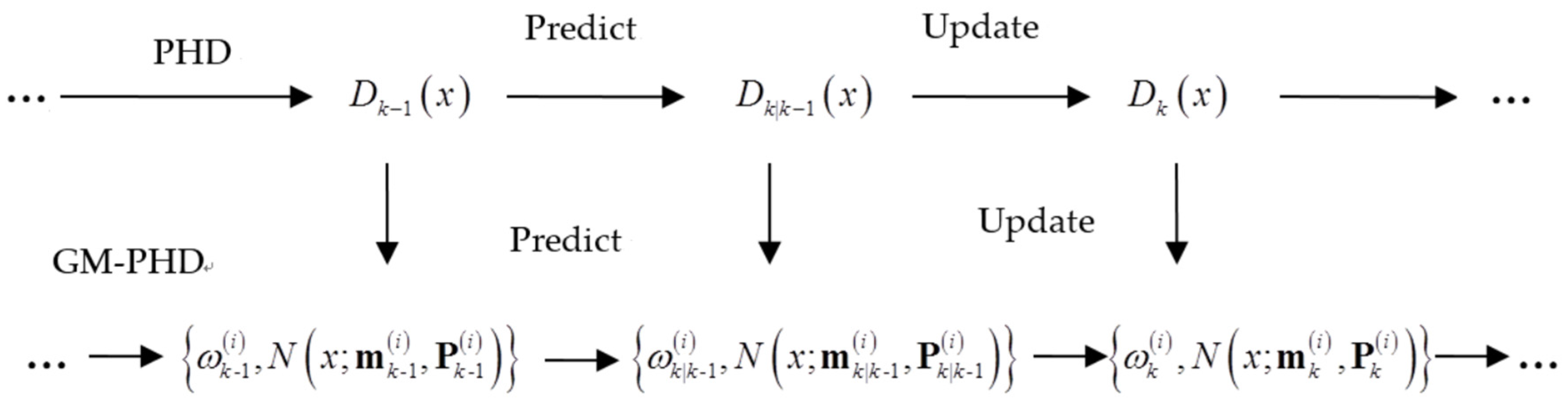
The PHD filter is a recursion algorithm that propagates the intensity function associated with the multi-targets posterior probability. To implement the PHD filter, under a linear target system, the Gaussian mixture (GM) method has been introduced in the PHD filter. Additionally, it forms the GM-PHD filter algorithm. The relationship between the PHD and GM-PHD is shown as in Figure 2.
In order to implement the GM-PHD filter algorithm, some additional assumptions of Gaussianmulti-targets model are required besides the PHD filter, which is described as below.
- A.1.
- The motion model and sensor measurement model are all linear Gaussian.where is the state transition matrix, is the measurement matrix, and and are the process noise covariance and measurement noise covariance respectively.
- A.2.
- The survival and detection probabilities for targets are state independent.
- A.3.
- The target birth RFS is also a Gaussian mixture of the form.where, , , , , are given parameters that determine the intensity of target birth; and , are calculated using Kalman filter [24], which are used in many parts in the paper.
Based on the assumption A.1–A.3, the posterior intensity at time k − 1 is a Gaussian mixture of the form in Equation (8). Here, the main prediction and update process of GM-PHD algorithm can be described as below.
Prediction:
where is given in Equation (7), is shown in Equation (10).
Update:
where, , , are shown in Equation (12).
For a more detailed mathematical derivation on GM-PHD filter, we can see it in literature [11]. The computational complexity of the PHD filtering algorithm is , where is the target number of tracking and is the cardinalized RFS measurement at each moment. Due to the interference of clutter, the GM-PHD filter algorithm has a large deviation and fluctuation in the estimation of the target number.
2.3. GM-CPHD Algorithm
Compared with the PHD filter, CPHD not only propagates the intensity function but also the cardinality distribution, which makes the estimation deviation of the target number small and the accuracy improved [25].The relationship between PHD and CPHD is shown in Figure 3.
To implement the CPHD filters, under linear target systems, the Gaussian mixture (GM) method has been introduced in CPHD. Based on the assumption A.1–A.3, the main prediction and update process of the GM-CPHD filter algorithm can be described as below.
Some general expressions are shown as below.
where is binomial coefficient, is the permutation coefficient, is the inner product, and is the elementary symmetric function of order for the finite real set of .
Prediction: suppose at time k − 1, the Gaussian mixture form of posterior intensity and posterior cardinality distribution are given. Then, the prediction are described by Equations (14) and (15), respectively.
where , are the same with which is shown in Equations (7) and (10), respectively.
Update:
where the parameters are shown as below in Equation (18).
For a more detailed mathematical derivation of the GM-CPHD filter, look to [17]. The computational complexity of the CPHD filtering algorithm is , where is the target number of tracking and is the cardinalized of RFS measurement at each moment. Compared with the GM-PHD filter, using the GM-CPHD filter, the estimation deviation of the target number is small and the tracking performance is improved.
3. The Proposed Algorithm Based on Novel Detection Probability
3.1. Gating Technical Strategy
In theory, the PHD and CPHD algorithms have a computational complexity order of /. We can see that the computational load can be reduced by reducing the cardinality of the RFS measurement. In literature [22], the elliptical gate is used in the GM-CPHD filter to reduce the cardinality of the RFS measurement, thereby reducing the computational burden, which is defined as Equation (19).
where is validate measurement set and is the threshold of tracking gate, which is depend on gate probability and measurement dimension , see in literature [22]. Since the elliptical gate may lead to target detection missing, the adaptive tracking gate proposed in literature [23] is as follows.
where is the predicted weight using a Gaussian mixture implementation of the filter.
3.2. An Novel Detection Probability Model
The design of the underwater target tracking should be linked with a sonar equation [26]. Here, the detection probability model is modeled through the active sonar equation. The active sonar equation is defined as below.
describing source level (SL), one-way transmission loss (TL), target strength (TS), environmental noise level (NL), direction index (DI) and detection threshold (DT). TL can be expressed as a function of distance, indirectly, and the signal-to-noise ratio (SNR) and the detection threshold can also be expressed as a function of distance. According to the theory of sonar detection, the relationship between SNR and detection probability and false alarm probability can be expressed by the receiver operating characteristic (ROC) curve. Therefore, the relationship between detection probability and distance can be modeled by the sonar equation and ROC curve.
According to the binary signal detection theory [27], the derivation process is described as follows and uses the two hypotheses as shown below.
where is known signal and is the Gaussian noise with mean zero and covariance . The discrete time series is obtained by for the sampling interval.
The likelihood ratio is denoted .
Simplifying the above Equation (23), we get the new Equation (24).
The left definition of the inequality is the detection statistic, and the right side is the test threshold , which can be determined by different discriminate criteria. At the same time, the above results are generalized to the general situation, , then the summation operation becomes integral operation and the statistical test quantity is . An equivalent test is shown as blow.
When is true, , .
When is true, , .
The probability density function of the test statistic is obtained under the condition of binary hypothesis, which are shown in Equation (26).
Therefore, the false detection probability and detection probability are as below, respectively.
From the equation above, we can get the detection probability, as defined blow.
where express the standard normal distribution, .
Assuming that the active detection method is adopted, the wave front is the cylindrical wave when distance is far away, . According to Equation (21), , combining Equation (28). The relationship between the detection probability, the false detection probability and the distance is shown in Equation (29).
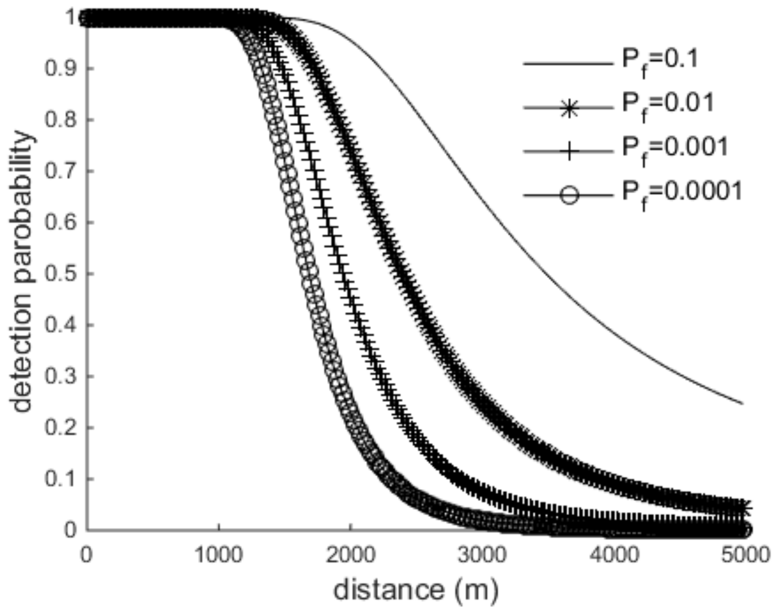
Given the uncertainty of the false detection probability, we cannot get the analytic relationship between the detection probability and distance, here choosing the Naiman Pearson criterion as the criterion. That is, the detection probability is maximized under the condition of false detection probability. When the false detection probability is fixed, we can get the analytic expression between the detection probability and target distance. Assuming the source level , the fifth grade sea condition ,, and ignoring the direction index , the relationship between the detection probability and the distance is shown in Figure 4.
It can be seen from Figure 4, when at a certain distance, the false detection probability is greater, the detection probability greater; when the detection probability is certain, the false detection probability is greater with the distance further. No matter how the false detection probability is chosen, the detection probability decreases with an increase in distance, and when the false detection probability is smaller, the detection probability decays faster.
3.3. The Proposed Algorithm with Novel Detection Probability
In order to implement the filter algorithm to the active sonar MTT system, we analyze the main process of prediction and update in GM-PHD algorithm. We can see from Equations (9)–(12), the detection probability is not involved in the prediction process, while the update process is infected by detection probability. The first item in Equation (11) is the estimation of the missing part, the second item is the target estimation originated from measurement. The detection probability shown in Equation (12) shows the trust of the measurement, namely, is bigger. The update results rely more so on the measurement, with a small effect with the estimation of the missing part. Otherwise, is smaller. The update results are rely more so on the estimation of the missing part, while a small effect on the measurement part. Therefore, these two items are a contradiction in each update processes; the detection probability will affect the update result. Hence, the proper detection probability can ensure reliable results. Similar results can get found from the analysis from the GM-CPHD algorithm. In traditional GM-PHD and GM-CPHD algorithms, we assume the detection probability is known a priori with a high detection probability, which is not suitable in practice. Here, with an adaptive elliptical gate, the proposed detection probability replaces the traditional detection probability, which is shown in Equation (30), all making the proposed algorithm perform accurately, as expected.
4. Simulation and Analysis
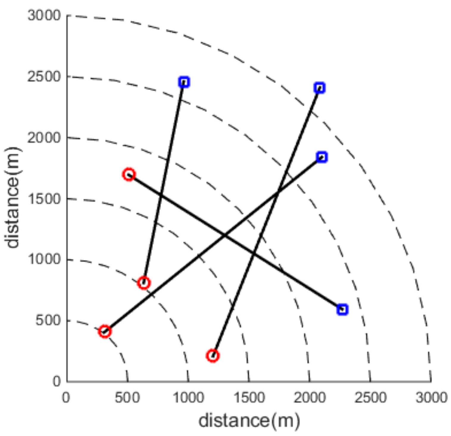
To evaluate the performance of the proposed algorithm, consider a two-dimensional scenario with an unknown and time-varying number of targets observed in clutter over the surveillance region . The sensor is located at the origin and the clutter is molded as a Poisson RFS with intensity (i.e., 10 clutter returns over surveillance region each scan). Each target has survival probability and follows a linear Gaussian dynamic motion with constant velocity. The target birth process is assumed to be a Poisson distribution with , with , , , , , and . The gate threshold is set to , which corresponds to a two-dimensional gating probability of and sampling interval s. The Gaussian mixture filter has a pruning threshold , merging threshold , and limitation on number of Gaussians . The state parameters of targets are shown in Table 1. The trajectory of targets are shown in Figure 5. The red circle represents the starting position of the target, and the blue box indicates the end position of the target, and the dotted line indicates the circle of the distance from the origin. The following simulation and analysis are all in the same scenario show in Figure 5.
4.1. Simulation and Analysis of GM-PHD and Pd-GM-PHD
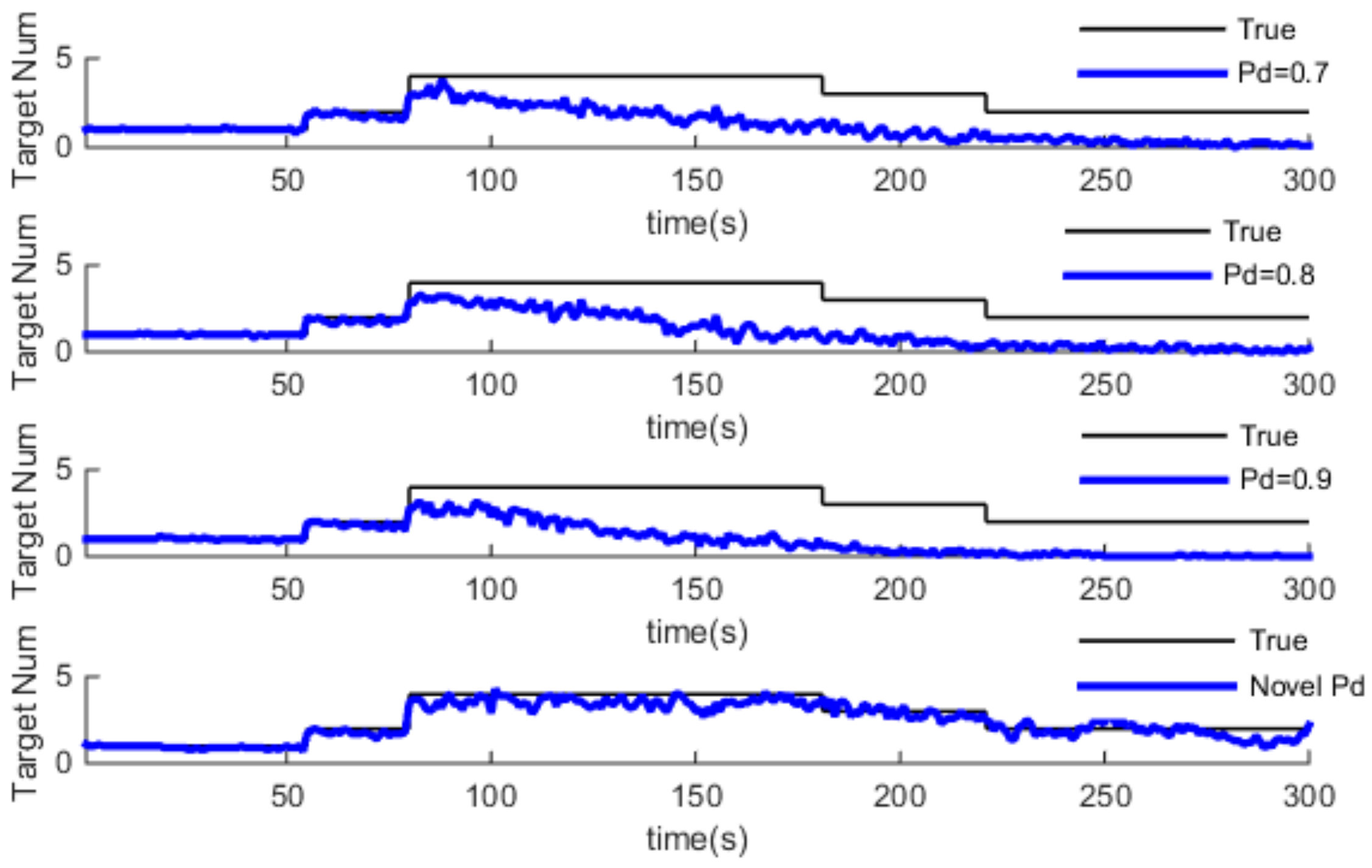
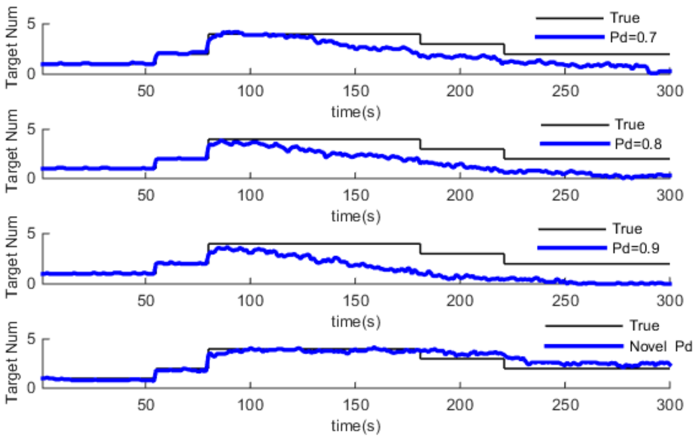
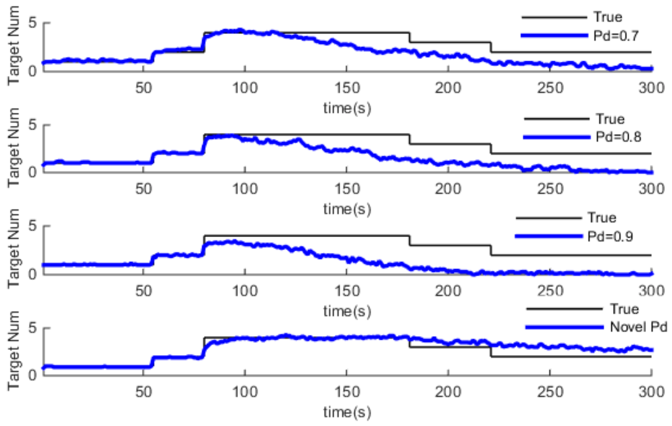
In this part, we use the same adaptive gating technical for the GM-PHD algorithm, then, we compare the GM-PHD algorithm with different constant detection probability and Pd-GM-PHD algorithm in a different clutter environment. Simulation results are shown in Figure 6, Figure 7 and Figure 8, which show the estimation of target number. Also, the average time Optimal Subpattern Assignment distance (OSPA) [28] is used to evaluate the performance of the algorithm, which is shown in Table 2.
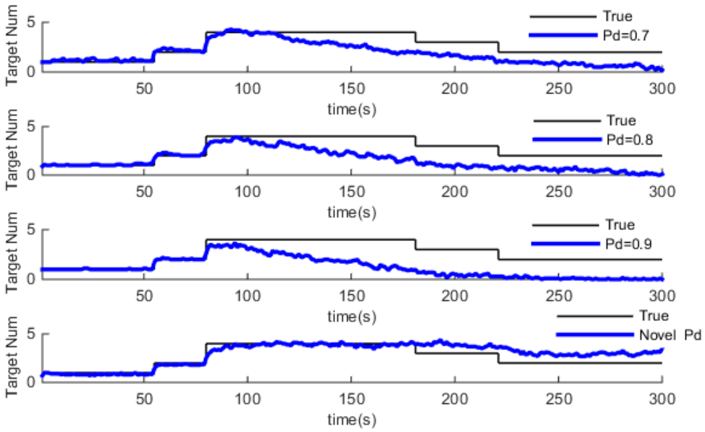
From Figure 6, Figure 7 and Figure 8, we can see that the GM-PHD filter algorithm with constant detection probability cannot estimate the target number accurately, while the estimation with Pd-GM-PHD can better approximated to the true target number. Also, after 80 s, the estimation of target number begins to deviate from the true value and there is a phenomenon that the higher detection probability, the greater the estimation of target number error. As the detection probability decreases with distance in practice, while the GM-PHD filter algorithm still believes that measurement is credible, eventually the estimation accuracy gets worse. As for the Pd-GM-PHD filter algorithm, the detection probability changes with distance, so its performance is better than the GM-PHD using the same adaptive gating technique with different constant detection probability.
Table 2 shows the average OSPA distance between GM-PHD with constant detection probability and novel detection probability in different clutter environments. In the update process in the GM-PHD filter algorithm, the detection probability will affect the update results. The detection probability will decrease with distance, then unreliable measurements have the high weight in the update process. So the higher detection probability, the worse the tracking performance is and the bigger the average OPSA distance is. While this phenomenon will improve when using the novel detection probability, which not only can make the estimation of target number more reliable, but also can improve the performance of tracking accuracy. So we can get the similar results with Figure 6, Figure 7 and Figure 8 that the Pd-GM-PHD has a good performance.
4.2. Simulation and Analysis of GM-CPHD and Pd-GM-CPHD
In this part, in order to verify the performance of proposed Pd-GM-CPHD algorithm, we use the same adaptive gating technical to GM-CPHD algorithm, and then compare two algorithms in different clutter environments. Simulation results of the estimation of target number are shown in Figure 9, Figure 10 and Figure 11. Also, the average time OSPA distance is used to evaluate the performance of the algorithm which is shown in Table 3.
From Figure 9, Figure 10 and Figure 11, we can see that estimation of target number is credible after 80 s. The estimated value obviously deviates from the true value when using GM-CPHD with constant detection probability. As the detection probability decreases with distance in practice, the higher the detection probability, the greater the estimation error of the target potential. On the contrary, a low detection probability performs better than a high detection probability, in which the reliability of the measurement decreases, and this leads the missing detection part to increase to remedy the update value, so the target number is more close to the true value. For the Pd-GM-CPHD algorithm, the detection probability changed with distance. However, when the target distance is more than 2km, the detection probability dropped to less 0.4. In this case, even the estimation of the target number deviates from the true value, but it still has a certain tracking ability. In general, the Pd-GM-CPHD algorithm is more accurate in estimating the target number.
Table 3 shows the average OSPA distance between GM-CPHD with constant detection probability and Pd-GM-CPHD under different clutter environment. Due to the detection probability decreasing with distance, the higher detection probability leads to the unreliable measurement being used to estimate the target state. So the tracking performance is reduced. The average OPSA distance is bigger. The Pd-GM-CPHD algorithm uses the adaptive detection probability, which not only can make the estimation of the target number more reliable but also can improve the performance of tracking accuracy. So we can get the similar results with Figure 9, Figure 10 and Figure 11 that the Pd-GM-CPHD have a good performance.
4.3. Simulation and Analysis of Different Three Algorithm
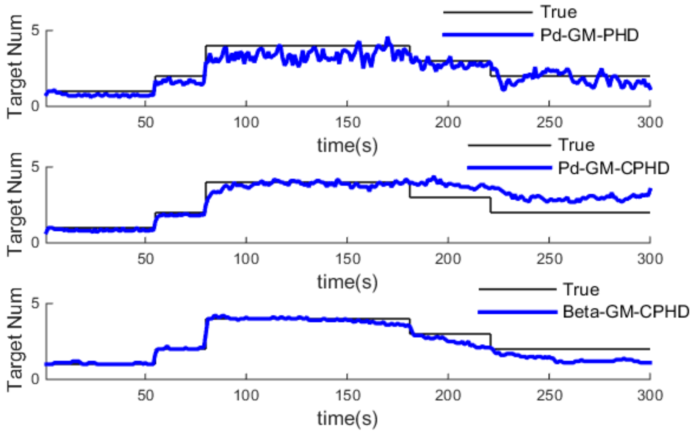
In this part, we compare the performance of Pd-GM-PHD, Pd-GM-CPHD and Beta-GM-CPHD in different clutter environments. Simulation results are shown in Figure 12, Figure 13 and Figure 14, which show the estimation of target number. Also, the average time OSPA distance is used to evaluate the performance of the algorithm, which is shown in Table 4. At the same time, statistical results are given in Table 5, in which the running time of three algorithms in different scenarios with an increase of clutter intensity is described.
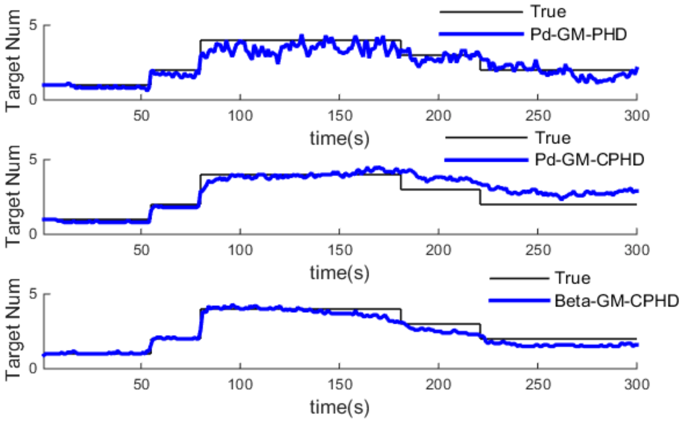
From Figure 12, Figure 13 and Figure 14, we can see that the three algorithms can get a good performance in estimating the target number in different clutter environments. This is due to fact the CPHD algorithm jointly propagates the intensity function and the cardinality distribution while PHD algorithm just propagates the intensity function. Hence, the Pd-GM-PHD algorithm has a bigger fluctuation than Pd-GM-CPHD and Beta-GM-CPHD in the estimation of the target number. As the detection probability decreases with distance, after 180 s, the detection probability affects the tracking performance even more; after 250 s, the detection probability is near 0.2, which causes a more unreliable measurement to be used to update the process in Pd-GM-CPHD algorithm, and also the Beta-GM-CPHD performs not as well.
Table 4 shows the average OSPA distance with three algorithms in different clutter environments. The smaller time average OSPA-distance is shown in the Pd-GM-CPHD algorithm in different clutter environments, which we can see in Table 4. Pd-GM-PHD is worse than Beta-GM-CPHD algorithm no matter the clutter intensity.
At the same time, the running time of three algorithms in different scenario is analysis and compared, statistical results are shown in Table 5. The PC platform is Intel (R) Core (TM) i5-4460, CPU @ 3.20 GHz, RAM 8.0 G, MATLAB (R2014b, The MathWorks, Inc., Natick, MA, USA, 2014)).
Table 5 shows that with the increase of the clutter intensity, the average running time of these algorithms will increase. Compared with Beta-GM-CPHD, the computational load of Pd-GM-PHD and Pd-GM-CPHD is very small, which makes sure it can be used in practice. Above all, the noveldetection probability proposed in this paper can get good performance in the GM-PHD and GM-CPHD algorithms with applications in underwater MTT systems.
5. Conclusions
In order to realize the underwater MTT problem, under linear Gaussian assumptions, we use the adaptive ellipse gate strategy to reduce the computational burden in GM-PHD and GM-CPHD algorithms. Also, we propose the novel detection probability which is modeled through the active sonar equation. Here, the adaptive ellipse gate strategy and novel detection probability are used in GM-PHD and GM-CPHD algorithms, which we call the Pd-GM-PHD algorithm and Pd-GM-CPHD algorithm. When using same adaptive gating technical to the GM-PHD algorithm and GM-CPHD algorithm, simulation results show that Pd-GM-PHD and Pd-GM-CPHD algorithms perform better in estimation of target number. Additionally, the tracking accuracy is improved compared to the GM-PHD and GM-CPHD algorithms. Furthermore, the proposed two algorithms are compared with Beta-GM-CPHD. The simulation results show that the novel detection probability used in GM-PHD and GM-CPHD algorithm is a good choice, which not only do better in the estimation of target number, but also more accurately in real applications.
Acknowledgments
This work is partially supported by NSFC (Natural Science Foundation of China), the NSFC number is 11574250, 51179157, 51409214, respectively. All authors gratefully acknowledge the helpful suggestions and comments from the editors and reviewers, this will be good for improve the paper.
Author Contributions
Xiao Chen and Yaan Li conceived and designed the experiments, Xiao Chen performed the experiments; Xiao Chen, Yuxing Li and Jing Yu analyzed the data, Xiao Chen wrote the manuscript. The authors have read, also approved the final manuscript.
Conflicts of Interest
The authors declare no conflicts of interest.
References
- Mallick, M.; Vo, B.-N.; Kirubarajan, T.; Arulampalam, S. Introduction to the Issue on Multitarget Tracking. IEEE J. Sel. Top. Signal Process. 2013, 7, 373–375. [Google Scholar] [CrossRef]
- Li, X.R.; Bar-Shalom, Y. Tracking in clutter with nearest neighbor filters: Analysis and performance. IEEE Trans. Aerosp. Electron. Syst. 1996, 32, 995–1010. [Google Scholar]
- Chen, X.; Li, Y.; Li, Y.; Yu, J.; Li, X. A Novel Probability Data Association for Target Tracking in a Clutter Environment. Sensors 2016, 16, 2180. [Google Scholar] [CrossRef] [PubMed]
- Habtemariam, B.; Tharmarasa, R.; Thayaparan, T.; Mallick, M.; Kirubarajan, T. A Multiple-Detection Joint Probabilistic Data Association Filter. IEEE J. Sel. Top. Signal Process. 2013, 7, 461–471. [Google Scholar] [CrossRef]
- Blackman, S.S. Multiple hypothesis tracking for multiple target tracking. IEEE Aerosp. Electron. Syst. Mag. 2004, 19, 5–18. [Google Scholar] [CrossRef]
- Lee, E.H.; Zhang, Q.; Song, T.L. Markov Chain Realization of Joint Integrated Probabilistic Data Association. Sensors 2017, 17, 2865. [Google Scholar] [CrossRef] [PubMed]
- Vo, B.-T.; Vo, B.-N.; Cantoni, A. Bayesian Filtering with Random Finite Set Observations. IEEE Trans. Signal Process. 2008, 56, 1313–1326. [Google Scholar] [CrossRef]
- Mahler, R. Multitarget Bayes Filtering via First-order Multitarget Moments. IEEE Trans. Aerosp. Electron. Syst. 2003, 39, 1152–1178. [Google Scholar] [CrossRef]
- Mahler, R. PHD filters of higher order in target number. IEEE Trans. Aerosp. Electron. Syst. 2007, 43, 1523–1543. [Google Scholar] [CrossRef]
- Vo, B.-N.; Singh, S.; Doucet, A. Sequential Monte Carlo methods for Multitarget Filtering with Random Finite Sets. IEEE Trans. Aerosp. Electron. Syst. 2005, 41, 1224–1245. [Google Scholar]
- Vo, B.-N.; Ma, W.-K. The Gaussian Mixture Probability Hypothesis Density Filter. IEEE Trans. Signal Process. 2006, 54, 4091–4104. [Google Scholar] [CrossRef]
- Vo, B.-T.; Vo, B.-N.; Cantoni, A. Analytic Implementations of the Cardinalized Probability Hypothesis Density Filter. IEEE Trans. Signal Process. 2007, 55, 3553–3567. [Google Scholar] [CrossRef]
- Vo, B.-T.; Vo, B.-N. Labeled random finite sets and multi-object conjugate priors. IEEE Trans. Signal Process. 2013, 61, 3460–3475. [Google Scholar] [CrossRef]
- Beard, M.; Reuter, S.; Granström, K.; Vo, B.-T.; Vo, B.-N.; Scheel, A. Multiple Extended Target Tracking with Labeled Random Finite Sets. IEEE Trans. Signal Process. 2016, 64, 1638–1653. [Google Scholar] [CrossRef]
- Nannuru, S.; Coates, M. Hybrid multi-Bernoulli and CPHD filters for superpositional sensors. IEEE Trans. Aerosp. Electron. Syst. 2015, 51, 2847–2863. [Google Scholar] [CrossRef]
- Schlangen, I.; Delande, E.D.; Houssineau, J.; Clark, D.E. A Second-Order PHD Filter with Mean and Variance in Target Number. IEEE Trans. Signal Process. 2018, 66, 48–63. [Google Scholar] [CrossRef]
- Tobias, M.; Lanterman, A.D. Probability Hypothesis Density-based Multitarget Tracking with Multiple Bistatic Range and Doppler Observations. IEE Proc. Radar Sonar Navig. 2005, 152, 195–205. [Google Scholar] [CrossRef]
- Clark, D.E.; Bell, J. Bayesian multiple target tracking in forward scan sonar images using the PHD filter. IEE Proc. Radar Sonar Navig. 2005, 152, 327–334. [Google Scholar] [CrossRef]
- Kalyan, B.; Balasuriya, A.; Wijesoma, S. Multiple target tracking in underwater sonar images using Particle-PHD filter. In Proceedings of the OCEANS 2006—Asia Pacific, Singapore, 16–19 May 2007. [Google Scholar]
- Hendeby, G.; Karlsson, R. Gaussian mixture PHD filtering with variable probability of detection. In Proceedings of the 2014 17th International Conference on Information Fusion (FUSION), Salamanca, Spain, 7–10 July 2014. [Google Scholar]
- Mahler, R.; Vo, B.-T.; Vo, B.-N. CPHD filtering with unknown clutter rate and detection profile. IEEE Trans. Signal Process. 2011, 59, 3497–3513. [Google Scholar] [CrossRef]
- Zhang, H.; Jing, Z.; Hu, S. Gaussian Mixture CPHD filter with Gating technique. Signal Process. 2009, 89, 1521–1530. [Google Scholar] [CrossRef]
- Macagnano, D.; De Abreu, G.T.F. Adaptive Gating for Multitarget Tracking with Gaussian Mixture filter. IEEE Trans. Signal Process. 2012, 60, 1533–1538. [Google Scholar] [CrossRef]
- Wang, X.; Fu, M.; Zhang, H. Target Tracking in Wireless Sensor Networks Based on the Combination of KF and MLE Using Distance Measurements. IEEE Trans. Mob. Comput. 2012, 11, 567–576. [Google Scholar] [CrossRef]
- El-Fallah, A.; Perloff, M. Multisensor-multitarget sensor management with target preference. Proc. SPIE 2004, 5429, 222–232. [Google Scholar]
- Tan, T. Sonar Technology; Harbin Engineering University Press: Harbin, China, 2009. [Google Scholar]
- Schonhoff, T.; Giordano, A. Detection and Estimation Theory and Its Application; Prentice Hall: Upper Saddle River, NJ, USA, 2007. [Google Scholar]
- Schumacher, D.; Vo, B.-T.; Vo, B.-N. A Consistent Metric for Performance Evaluation of Multi-Object Filters. IEEE Trans. Signal Process. 2008, 56, 3447–3457. [Google Scholar] [CrossRef]
Figure 1.
The space model of multi-targets tracking.
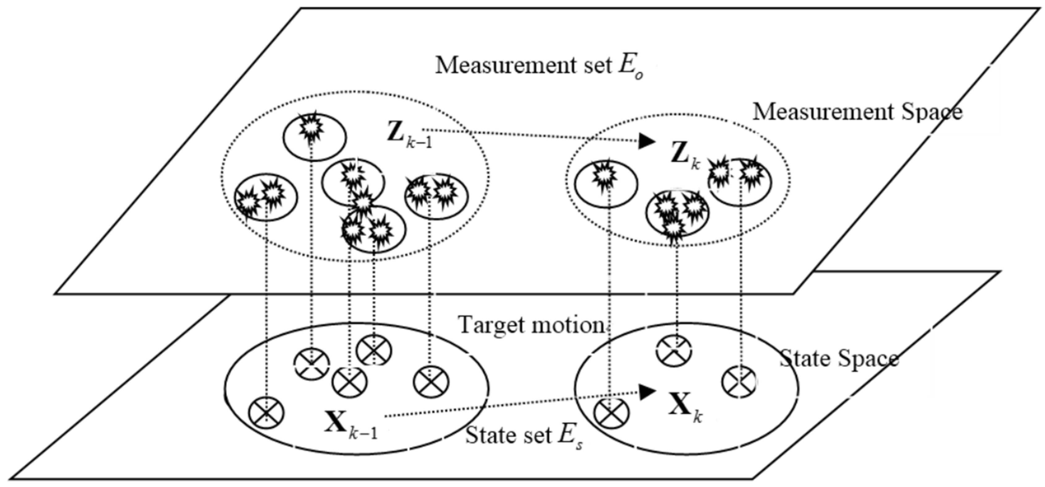
Figure 2.
Relationship between Probability Hypothesis Density (PHD) and Gaussian Mixture Probability Hypothesis Density (GM-PHD).
Figure 2.
Relationship between Probability Hypothesis Density (PHD) and Gaussian Mixture Probability Hypothesis Density (GM-PHD).

Figure 3.
Relationship between PHD and CPHD.
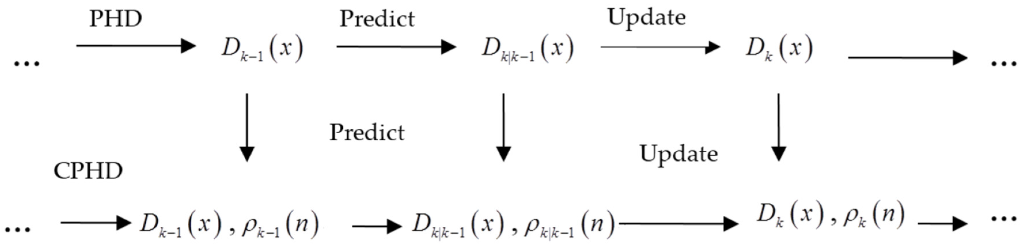
Figure 4.
Detection probability changes with distance.

Figure 5.
Trajectory of four target in two dimensional scenario.

Figure 6.
Comparison of target number estimation with different in clutter intensity .
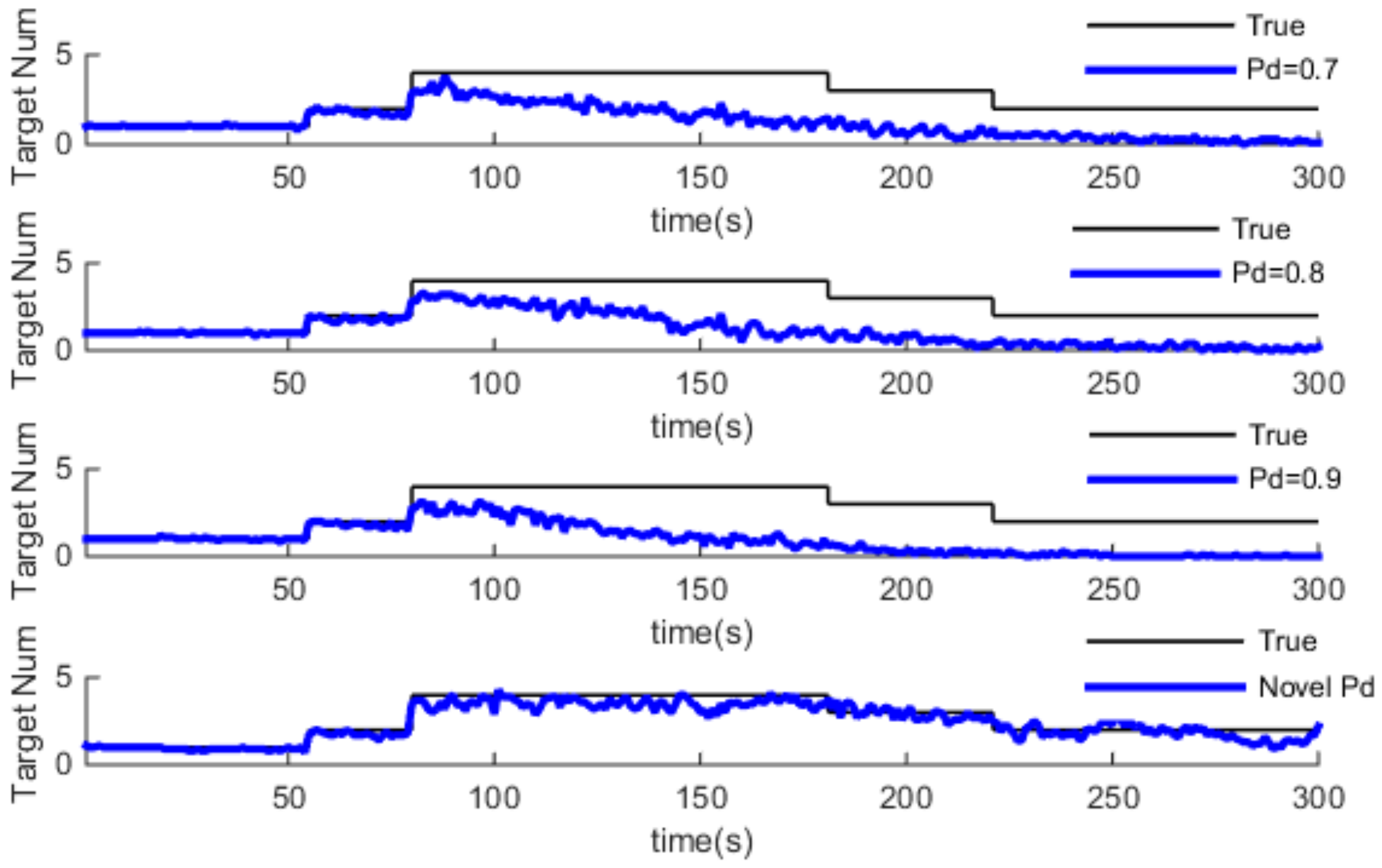
Figure 7.
Comparison of target number estimation with different in clutter intensity .

Figure 8.
Comparison of target number estimation with different in clutter intensity .
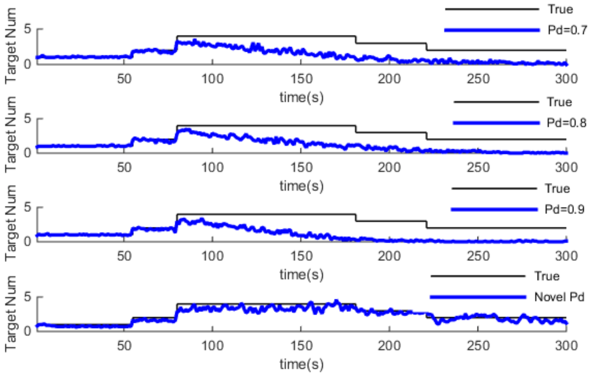
Figure 9.
Comparison of target number estimation with different in clutter intensity .

Figure 10.
Comparison of target number estimation with different in clutter intensity .

Figure 11.
Comparison of target number estimation with different in clutter intensity .

Figure 12.
Comparison of target number estimation in clutter intensity .
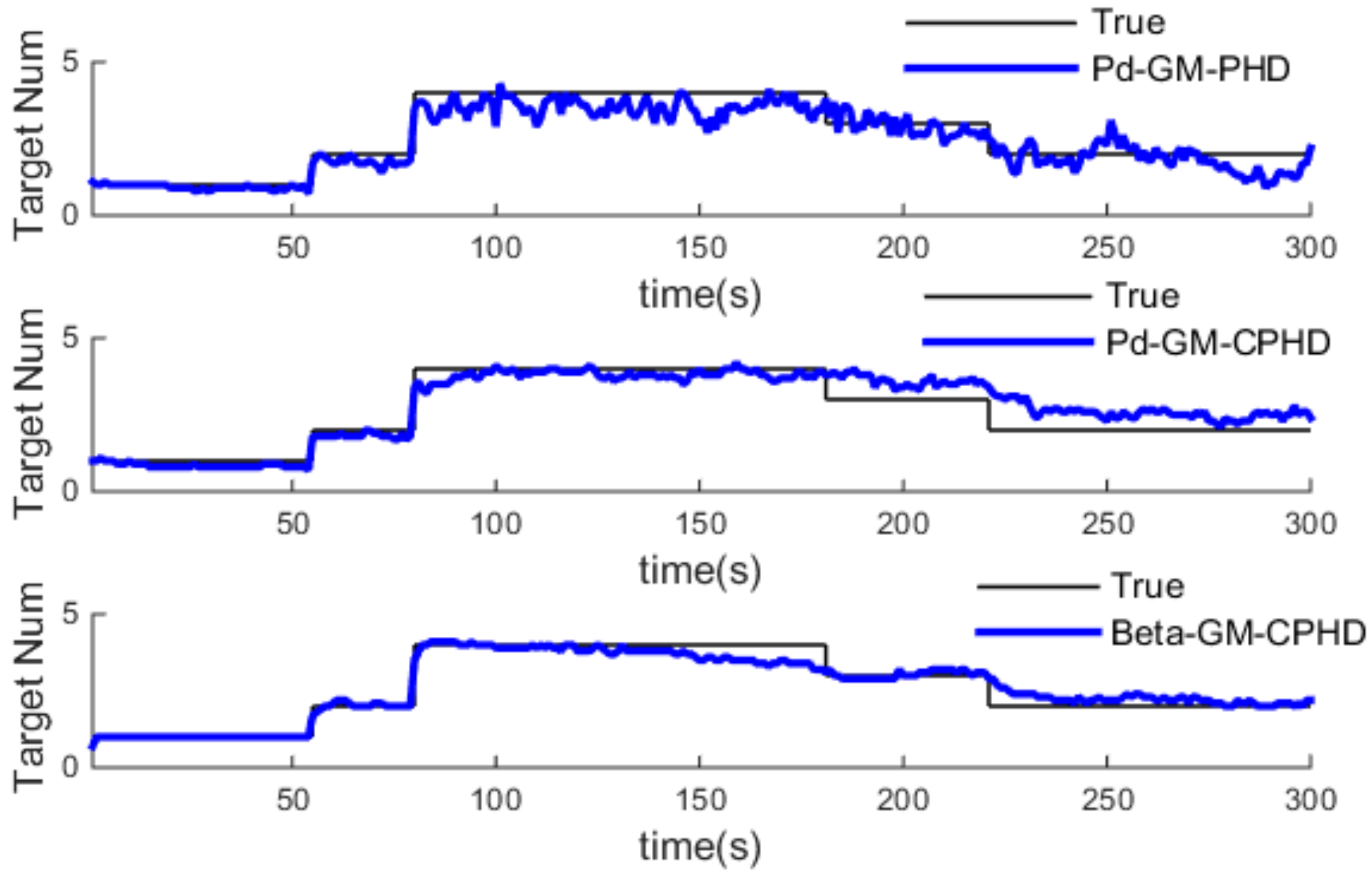
Figure 13.
Comparison of target number estimation in clutter intensity .

Figure 14.
Comparison of target number estimation in clutter intensity .

Table 1.
The state parameters of targets.
| State | Initial State | Start Time (s) | End Time (s) | |
|---|---|---|---|---|
| Target | ||||
| target 1 | (300 m, 10 m/s, 400 m, 8 m/s) | |||
| target 2 | (630 m, 2 m/s, 800 m, 10 m/s) | |||
| target 3 | (500 m, 8 m/s, 1700 m, −5 m/s) | |||
| target 4 | (1200 m, 4 m/s, 200 m, 10 m/s) | |||
Table 2.
Comparison of time average Optimal Subpattern Assignment distance (OSPA-distance, m) in different clutter environment. GM-PHD: Gaussian Mixture Probability Hypothesis Density.
Table 2.
Comparison of time average Optimal Subpattern Assignment distance (OSPA-distance, m) in different clutter environment. GM-PHD: Gaussian Mixture Probability Hypothesis Density.
| Time Average OSPA-Distance (m) | GM-PHD | Pd-GM-PHD | ||
|---|---|---|---|---|
| 53.4 | 55.19 | 61.57 | 35.26 | |
| 54.96 | 56.58 | 62.33 | 37.34 | |
| 55.54 | 57.66 | 63.25 | 41.51 | |
Table 3.
Comparison of time average OSPA-distance (m) in different clutter environments. GM-CPHD: Gaussian Mixture Cardinalized Probability Hypothesis Density.
Table 3.
Comparison of time average OSPA-distance (m) in different clutter environments. GM-CPHD: Gaussian Mixture Cardinalized Probability Hypothesis Density.
| Time Average OSPA-Distance (m) | GM-CPHD | Pd-GM-CPHD | ||
|---|---|---|---|---|
| 34.04 | 43.34 | 52.04 | 25.22 | |
| 39.29 | 46.61 | 55.63 | 26.54 | |
| 40.29 | 47.63 | 56.18 | 30.05 | |
Table 4.
Comparison of time average OSPA-distance (m) in different clutter environments.
| Time Average OSPA-Distance (m) | Pd-GM-PHD | Pd-GM-CPHD | Beta-GM-CPHD |
|---|---|---|---|
| 35.26 | 25.22 | 30.94 | |
| 37.34 | 26.54 | 34.7 | |
| 41.51 | 30.05 | 35.18 |
Table 5.
The average running time when tracking four targets (s).
| Clutter Intensity | Pd-GM-PHD | Pd-GM-CPHD | Beta-GM-CPHD |
|---|---|---|---|
| 2.86 | 5.76 | 44.32 | |
| 3.17 | 6.57 | 51.15 | |
| 4.48 | 10.55 | 69.35 |
© 2017 by the authors. Licensee MDPI, Basel, Switzerland. This article is an open access article distributed under the terms and conditions of the Creative Commons Attribution (CC BY) license (http://creativecommons.org/licenses/by/4.0/).
Share and Cite
MDPI and ACS Style
Chen, X.; Li, Y.; Li, Y.; Yu, J. PHD and CPHD Algorithms Based on a Novel Detection Probability Applied in an Active Sonar Tracking System. Appl. Sci. 2018, 8, 36. https://doi.org/10.3390/app8010036
AMA Style
Chen X, Li Y, Li Y, Yu J. PHD and CPHD Algorithms Based on a Novel Detection Probability Applied in an Active Sonar Tracking System. Applied Sciences. 2018; 8(1):36. https://doi.org/10.3390/app8010036
Chicago/Turabian StyleChen, Xiao, Yaan Li, Yuxing Li, and Jing Yu. 2018. "PHD and CPHD Algorithms Based on a Novel Detection Probability Applied in an Active Sonar Tracking System" Applied Sciences 8, no. 1: 36. https://doi.org/10.3390/app8010036
Note that from the first issue of 2016, this journal uses article numbers instead of page numbers. See further details here.