A Simplified Approach to Identify Sectional Deformation Modes of Thin-Walled Beams with Prismatic Cross-Sections

Featured Application

The simplified approach, along with the derived one-dimensional higher-order model, possesses efficiency and accuracy which makes it an alternative to the more sophisticated shell finite elements in the numerical analyses of thin-walled structures.

Abstract

In this paper, a simplified approach to identify sectional deformation modes of prismatic cross-sections is presented and utilized in the establishment of a higher-order beam model for the dynamic analyses of thin-walled structures. The model considers the displacement field through a linear superposition of a set of basis functions whose amplitudes vary along the beam axis. These basis functions, which describe basis deformation modes, are approximated from nodal displacements on the discretized cross-section midline, with interpolation polynomials. Their amplitudes acting in the object vibration shapes are extracted through a modal analysis. A procedure similar to combining like terms is then implemented to superpose basis deformation modes, with equal or opposite amplitude, to produce primary deformation modes. The final set of the sectional deformation modes are assembled with primary deformation modes, excluding the ones constituting conventional modes. The derived sectional deformation modes, hierarchically organized and physically meaningful, are used to update the basis functions in the higher-order beam model. Numerical examples have also been presented and the comparison with ANSYS shell model showed its accuracy, efficiency, and applicability in reproducing three-dimensional behaviors of thin-walled structures.

1. Introduction

Thin-walled structures are commonly used in civil, aeronautical, and mechanical engineering structures. For simplicity and computational efficiency, one-dimensional theories are preferred to two- and three-dimensional models. However, the development of an efficient one-dimensional theory faces a fundamental challenge of finding a general and simple procedure to determine the cross-section deformation modes capable of describing cross-section in-plane (distortion) and out-of-plane (warping) deformations [1]. Moreover, the set of deformation modes should have a hierarchic capability, to obtain a reduced model and a clear physical interpretation of structural behaviors.

To support this, several trends of enhancing beam theories have been developed in the last decades. Yu and Hodges [2,3] developed an asymptotic method and contributed much to variational asymptotic beam sectional analyses. Expansion of the beam displacement field through Taylor or Maclaurin series is a general approach to model both thin-walled and solid structures, and has branched out to composite structures, due to the work of Carrera and Pagani [4,5]. Saint-Venant-driven models have been widely studied from the beginning, and new developments can be referred to Morandini et al. [6], and Naccache and Fatmi [7]. Umansky and Vlasov were the pioneers in the research of thin-walled structures. Vlasov [8] established a general thin-walled beam theory with warping of open cross-sections considered. Warping of closed cross-sections was first described by Umansky [9] in his study of non-uniformed torsion of thin-walled beams. Since then, refinement of their thin-walled theories has been extensively studied and generated many achievements, such as the recent work of Kim et al. [10] and Kovvali et al. [11]. Some special structural behaviors, exhibiting their importance in engineering, were also studied where shear deformation was considered. These include the studies of multi-cell distortion (Gonçalves et al. [12]), warping due to shear-lag effects (Chen et al. [13]) and other secondary effects (Lacidogna [14], Seguy et al. [15], Lacalle et al. [16]). Additionally, there are also some studies focused on the physical interpretation of cross-section deformation modes [17,18].

Recently, the generalized beam theory (GBT) has been the subject of intense scholarly debate, which can accurately handle cross-section deformation stemming from the so-called GBT cross-section analysis. Since the groundbreaking work of Schardt [19], GBT has been developed to account for both warping and distortion with shear deformation [20] and transverse extension included; it has also been applied to multi-cell cross-sections [21], composite materials [22] and curved members [23]. As a comparable theory, the beam model, based on generalized eigenvectors [24,25] has been obtained by considering a mixed Hellinger-Reissner variational formulation. Its sectional deformation modes have been defined through a cross-section discretization, using two-dimensional elements. Vieira et al. [26,27] have also recently proposed a remarkable higher-order one-dimensional model, which allows one to accurately reproduce three-dimensional behaviors of thin-walled structures. The key point is the application of a criterion to uncouple governing equations which have been established based on the solution of a generalized eigenvalue problem. In all fairness, the three theories mentioned above are powerful enough to deal with almost any arbitrary thin-walled cross-sections and any mechanical analyses (including static, dynamic, bulking, and so on), with an acceptable and optional precision. However, one common problem is the solution of the generalized eigenvalue problem, which is quite involved and demanding in uncoupling cross-sectional deformation modes. Actually, a simplified approach that does not include all the features but has a high precision, is more suitable, in some cases.

In this paper, a one-dimensional model of thin-walled structures is presented with a simplified approach to identify sectional deformation modes of prismatic cross-sections. The paper is organized as follows. First, the one-dimensional governing differential equation of a prismatic thin-walled member is obtained, in Section 2. The cross-section analysis is then implemented, in Section 3, producing a set of basis deformation modes. A procedure similar to combining like terms is carried out next to identify the final set of sectional deformation modes, based on the data of the modal analysis, in Section 4. The derived sectional deformation modes are used to update the basis functions in the higher-order beam model. Subsequently, numerical examples are presented to validate the new approach, in Section 5. Finally, the main conclusions are outlined.

2. One-Dimensional Formulation

2.1. Displacement and Deformation Fields

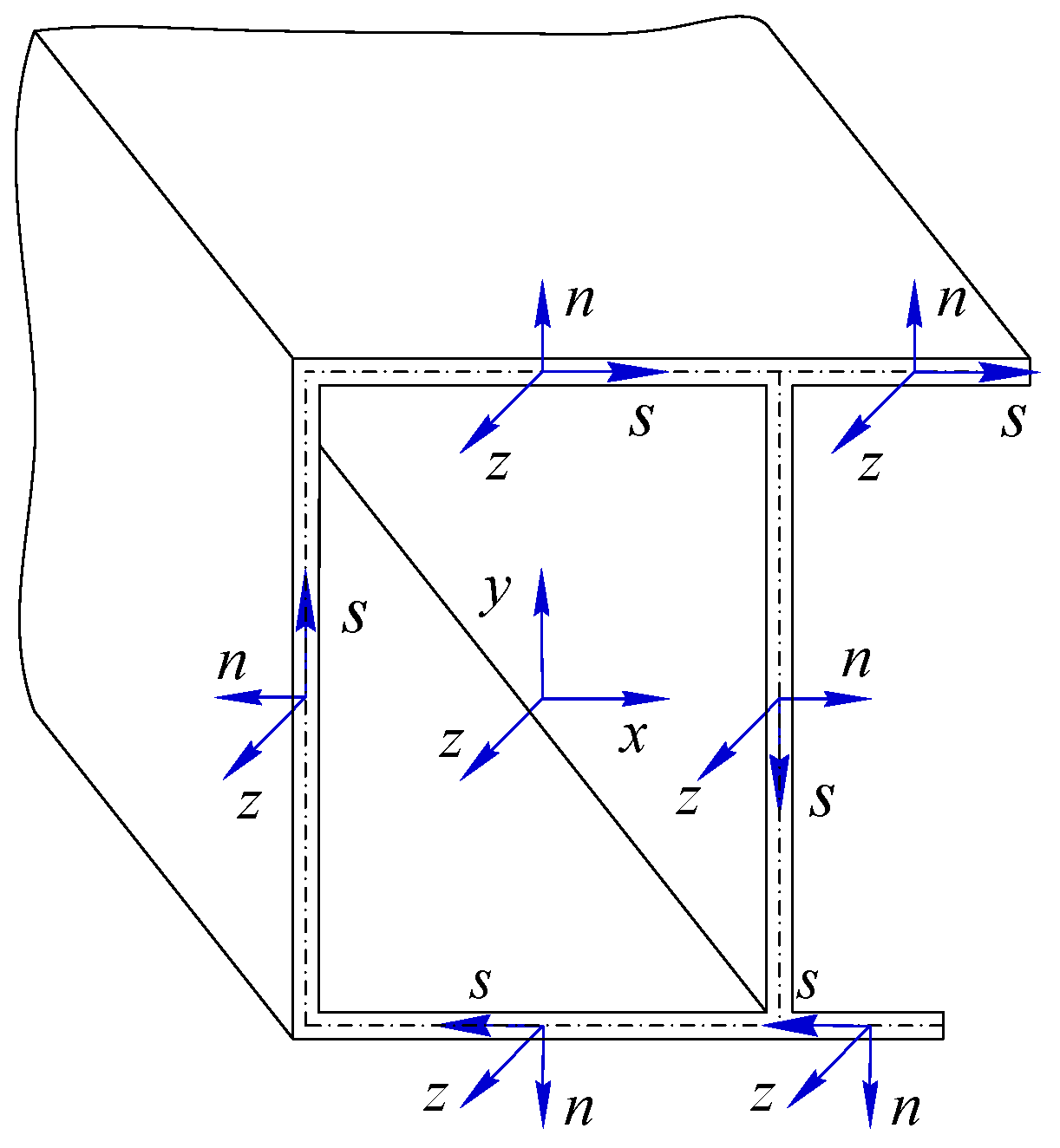
Consider a prismatic thin-walled structure depicted in Figure 1. The displacement of a point on the midline of the cross-section is defined in terms of the axial u, tangential v, and normal w components, which are defined to be positive, along the axes of the local coordinate system (n, s, z), adopted on each wall, respectively. The global coordinate system (x, y, z) with its origin located on the centroid of the cross-section of the beam end is also shown.

The displacement field U = [U_z(n, s, z), U_s(n, s, z), U_n(n, s, z)]^T considering both membrane and flexural behaviors of thin-walled structures is defined as

$$U_z\left(n,s,z\right)=u\left(s,z\right)-n\frac{\partial w\left(s,z\right)}{\partial z}, U_s\left(n,s,z\right)=v\left(s,z\right)-n\frac{\partial w\left(s,z\right)}{\partial s}, U_n\left(n,s,z\right)=w\left(s,z\right)$$

(1)

where the displacement variables u(s, z), v(s, z), and w(s, z) are separately approximated with a set of linearly independent basis functions, defined over the cross-section. This approximation separates the variable dependencies in z and s direction. The displacement field on the cross-section midline, u = [u(s, z), v(s, z), w(s, z)]^T, is thus approximated as follows:

$$u\left(s,z\right)={\mathsf{\Psi }}_{1}x, v\left(s,z\right)={\mathsf{\psi }}_{2}x, w\left(s,z\right)={\mathsf{\psi }}_{3}x$$

(2)

where Ψ₁ = [φ₁(s), φ₂(s), …, φ_N(s)], Ψ₂ = [ψ₁(s), ψ₂(s), …, ψ_N(s)], and Ψ₃ = [ω₁(s), ω₂(s), …, ω_N(s)] correspond to the sets of N basis functions, while for x = [χ₁(z), χ₂(z), …, χ_N(z)]^T, the generalized displacement χ_i(z) represents the axial variation of N₁ out-of-plane and N₂ in-plane deformation amplitudes; N = N₁ + N₂.

The three-dimensional displacement U can be expressed with a transformation matrix H = [H₁^T, H₂^T, H₃^T]^T as

$$U_z\left(n,s,z\right)=H_{1}u, U_s\left(n,s,z\right)=H_{2}u, U_n\left(n,s,z\right)=H_{3}u$$

(3)

where H₁ = [0, 1, −n∂/∂z], H₂ = [1, 0, −n∂/∂s] and H₃ = [0, 0, 1].

Neglecting defect and material uncertainty, the deformation field ε = [ε_zz(n, s, z), ε_ss(n, s, z), γ_sz(n, s, z)]^T and the corresponding stress field σ = [σ_zz(n, s, z), σ_ss(n, s, z), τ_sz(n, s, z)]^T are obtained under the small displacement hypothesis:

$$\mathsf{\epsilon }=CU=\left[\begin{array}{ccc}\frac{\partial }{\partial z}& 0& 0\\ 0& \frac{\partial }{\partial s}& 0\\ \frac{\partial }{\partial s}& \frac{\partial }{\partial z}& 0\end{array}\right]U, \mathsf{\sigma }=\mathbf{E}\mathsf{\epsilon }=\left[\begin{array}{ccc}\frac{E}{1-{\nu }^2}& \frac{E\nu }{1-{\nu }^2}& 0\\ \frac{E\nu }{1-{\nu }^2}& \frac{E}{1-{\nu }^2}& 0\\ 0& 0& \frac{E}{2\left(1+\nu \right)}\end{array}\right]\mathsf{\epsilon }$$

(4)

where C is the compatibility operator and E is the constitutive matrix of the plate in plane stress condition; E and ν are the Young’s modulus and Poisson’s ratio of the material, respectively.

2.2. Governing Equations

The beam energy components are essential for the application of Hamilton’s principle, including the strain energy, the potential energy, and the kinetic energy. By definition, they are separately given by the following equations.

$$U=\frac{1}{2}{\displaystyle \underset{V}{\iiint }{\mathsf{\epsilon }}^{\mathrm{T}}\mathsf{\sigma }\mathrm{d}V}=\frac{1}{2}{\displaystyle \underset{L}{\int }{\displaystyle \underset{A}{\int }{x}^{\mathrm{T}}{\mathsf{\psi }}^{\mathrm{T}}{H}^{\mathrm{T}}{c}^{\mathrm{T}}EcH\mathsf{\psi }x\mathrm{d}A\mathrm{d}z}}$$

(5)

$$U_{\mathrm{P}}=-{\displaystyle \underset{L}{\int }{\displaystyle \underset{A}{\int }{U}^{\mathrm{T}}}}p\mathrm{d}A\mathrm{d}z-{{\displaystyle \underset{A}{\int }\left[U^{\mathrm{T}}p\right]}}_{z=z_1}^{z=z_2}\mathrm{d}A=-{\displaystyle \underset{L}{\int }{x}^{\mathrm{T}}{\mathsf{\psi }}^{\mathrm{T}}{H}^{\mathrm{T}}p\mathrm{d}z}-{\left[x^{\mathrm{T}}{\mathsf{\psi }}^{\mathrm{T}}{H}^{\mathrm{T}}\overline{\mathsf{\sigma }}\right]}_{z=z_1}^{z=z_2}$$

(6)

$$T=\frac{1}{2}{\displaystyle \underset{V}{\iiint }\rho \frac{\partial U^{\mathrm{T}}}{\partial t}\frac{\partial U}{\partial t}\mathrm{d}V}=\frac{1}{2}{\displaystyle \underset{L}{\int }{\displaystyle \underset{A}{\int }\frac{\partial x^{\mathrm{T}}}{\partial t}{\mathsf{\psi }}^{\mathrm{T}}{H}^{\mathrm{T}}\rho H\mathsf{\psi }\frac{\partial x}{\partial t}\mathrm{d}A\mathrm{d}z}}$$

(7)

where V, A and L are the volume, the cross-section area and the length of the structure, respectively; ρ is material density; p denotes the loading vector consisting of distributed loads in the axial, tangential, and normal directions; coordinates z₁ and z₂ (z₁ < z₂) represent the axial coordinates of the two ends of the thin-walled structure and $\overline{\mathsf{\sigma }}$ indicates the strain vector imposed at the ends.

The formulation of the dynamic governing equation involves the application of Hamilton principle:

$$\delta {\displaystyle \underset{t_1}{\overset{t_2}{\int }}{L}_{\mathrm{a}}\mathrm{d}t}=0$$

(8)

where L_a is the Lagrangian defined as L_a = T − U − U_P in this paper, and t₁ and t₂ are the start and end times, respectively.

Substituting Equations (5)–(7) into Equation (8) and applying the integration by parts, by imposing the condition

$$\delta {x|}_{t=t_1}=\delta {x|}_{t=t_2}=0$$

(9)

yields

$$\begin{array}{cc}\hfill \delta H& =-{\displaystyle \underset{t_1}{\overset{t_2}{\int }}\left[{\displaystyle \underset{L}{\int }{\displaystyle \underset{A}{\int }\delta x^{\mathrm{T}}{\mathsf{\psi }}^{\mathrm{T}}{H}^{\mathrm{T}}\eta H\mathsf{\psi }\frac{{\partial }^{2}x}{\partial t^2}\mathrm{d}A\mathrm{d}z}}\right]\mathrm{d}t}-{\displaystyle \underset{t_1}{\overset{t_2}{\int }}\left[{\displaystyle \underset{L}{\int }{\displaystyle \underset{A}{\int }\delta x^{\mathrm{T}}{\mathsf{\psi }}^{\mathrm{T}}{H}^{\mathrm{T}}{c}^{\mathrm{T}}EcH\mathsf{\psi }x\mathrm{d}A\mathrm{d}z}}\right]\mathrm{d}t}\hfill \\ & \hspace{1em}\hspace{1em}+{\displaystyle \underset{t_1}{\overset{t_2}{\int }}\left[{\displaystyle \underset{L}{\int }{\displaystyle \underset{A}{\int }\delta x^{\mathrm{T}}{\mathsf{\psi }}^{\mathrm{T}}{H}^{\mathrm{T}}p\mathrm{d}A\mathrm{d}z}}+{\displaystyle \underset{A}{\int }{\left[\delta x^{\mathrm{T}}{\mathsf{\psi }}^{\mathrm{T}}{H}^{\mathrm{T}}\overline{\mathsf{\sigma }}\right]}_{z=z_1}^{z=z_2}\mathrm{d}A}\right]}\mathrm{d}t\hfill \\ & =0\hfill \end{array}$$

(10)

The dynamic governing equation of the thin-walled structure can then be derived as

$$\begin{array}{c}{\displaystyle \underset{L}{\int }{\displaystyle \underset{A}{\int }\delta x^{\mathrm{T}}{\mathsf{\psi }}^{\mathrm{T}}{H}^{\mathrm{T}}\eta H\mathsf{\psi }\frac{{\partial }^{2}x}{\partial t^2}\mathrm{d}A\mathrm{d}z}}+{\displaystyle \underset{L}{\int }{\displaystyle \underset{A}{\int }\delta x^{\mathrm{T}}{\mathsf{\psi }}^{\mathrm{T}}{H}^{\mathrm{T}}{c}^{\mathrm{T}}EcH\mathsf{\psi }x\mathrm{d}A\mathrm{d}z}}\\ -{\displaystyle \underset{L}{\int }{\displaystyle \underset{A}{\int }\delta x^{\mathrm{T}}{\mathsf{\psi }}^{\mathrm{T}}{H}^{\mathrm{T}}p\mathrm{d}A\mathrm{d}z}}-{\displaystyle \underset{A}{\int }{\left[\delta x^{\mathrm{T}}{\mathsf{\psi }}^{\mathrm{T}}{H}^{\mathrm{T}}\overline{\mathsf{\sigma }}\right]}_{z=z_1}^{z=z_2}\mathrm{d}A}=0\end{array}$$

(11)

2.3. Finite Element Implementation

The finite element method is employed in this paper for the ease of computation. In consideration of the second-order partial derivative in Equation (11), the quadratic interpolation function is used to approximate the axial displacement field within an element.

$$x=NX=\left[\begin{array}{ccc}{N}_1& N_2& N_3\end{array}\right]X$$

(12)

where N and X represent the shape function matrix and the nodal generalized displacement vector, respectively. The submatrices in Equation (12) are written as follows:

$$N_1=\left(\frac{2z^2}{l^2}-\frac{3z}{l}+1\right)I_N, N_2=\left(\frac{4z}{l}-\frac{4z^2}{l^2}\right)I_N, N_3=\left(\frac{2z^2}{l^2}-\frac{z}{l}\right)I_N$$

(13)

where the coordinate z varies from 0 to l within an element, and I_N denotes the N × N identity matrix. The vector X in Equation (12) is divided into three submatrices.

$$X={\left[\begin{array}{ccc}{X}_1^{\mathrm{T}}& X_2^{\mathrm{T}}& X_3^{\mathrm{T}}\end{array}\right]}^{\mathrm{T}}, X_i={\left[\begin{array}{cccc}{X}_{1\left(i\right)}& X_{2\left(i\right)}& \cdots & X_{N\left(i\right)}\end{array}\right]}^{\mathrm{T}}, i=1, 2, 3$$

(14)

where the subscripts 1, 2, and 3 indicate two end and one middle nodes of an element. Specially,

$$\begin{gathered} {\displaystyle \underset{A}{\int }{\left[x^{\mathrm{T}}{\mathsf{\psi }}^{\mathrm{T}}{H}^{\mathrm{T}}\overline{\mathsf{\sigma }}\right]}_{z=z_1}^{z=z_2}\mathrm{d}A}={\displaystyle \underset{A}{\int }{\left[x^{\mathrm{T}}\right]}_{z=z_2}{\mathsf{\psi }}^{\mathrm{T}}{H}^{\mathrm{T}}{\left[\overline{\mathsf{\sigma }}\right]}_{z=z_2}\mathrm{d}A}-{\displaystyle \underset{A}{\int }{\left[x^{\mathrm{T}}\right]}_{z=z_1}{\mathsf{\psi }}^{\mathrm{T}}{H}^{\mathrm{T}}{\left[\overline{\mathsf{\sigma }}\right]}_{z=z_1}\mathrm{d}A} \\ ={\displaystyle \underset{A}{\int }{X}_3^{\mathrm{T}}{\mathsf{\psi }}^{\mathrm{T}}{H}^{\mathrm{T}}{\left[\overline{\mathsf{\sigma }}\right]}_{z=z_2}\mathrm{d}A}-{\displaystyle \underset{A}{\int }{X}_1^{\mathrm{T}}{\mathsf{\psi }}^{\mathrm{T}}{H}^{\mathrm{T}}{\left[\overline{\mathsf{\sigma }}\right]}_{z=z_1}\mathrm{d}A}={\displaystyle \underset{A}{\int }{X}^{\mathrm{T}}{\left[{\overline{N}}^{\mathrm{T}}{\mathsf{\psi }}^{\mathrm{T}}{H}^{\mathrm{T}}\overline{\mathsf{\sigma }}\right]}_{z=z_1}^{z=z_2}\mathrm{d}A} \end{gathered}$$

(15)

where ${\left[{\overline{N}}^{\mathrm{T}}\right]}_{z=z_2}=\left[O_N,O_N,I_N\right]$, ${\left[{\overline{N}}^{\mathrm{T}}\right]}_{z=z_1}=\left[I_N,O_N,O_N\right]$ and O_N denotes the N × N null matrix.

Substituting Equations (12) and (15) into Equation (11), and referring to the relationship below:

$$\delta x^{\mathrm{T}}\ne 0 \Rightarrow \delta X^{\mathrm{T}}\ne 0$$

(16)

leads to the following element formulation

$${\displaystyle \underset{L}{\int }{\displaystyle \underset{A}{\int }{N}^{\mathrm{T}}{\mathsf{\psi }}^{\mathrm{T}}{H}^{\mathrm{T}}\eta H\mathsf{\psi }\frac{{\partial }^{2}X}{\partial t^2}\mathrm{d}A\mathrm{d}z}}+{\displaystyle \underset{L}{\int }{\displaystyle \underset{A}{\int }{N}^{\mathrm{T}}{\mathsf{\psi }}^{\mathrm{T}}{H}^{\mathrm{T}}{c}^{\mathrm{T}}EcH\mathsf{\psi }X\mathrm{d}A\mathrm{d}z}}-{\displaystyle \underset{L}{\int }{\displaystyle \underset{A}{\int }{N}^{\mathrm{T}}{\mathsf{\psi }}^{\mathrm{T}}{H}^{\mathrm{T}}p\mathrm{d}A\mathrm{d}z}}-{\displaystyle \underset{A}{\int }{\left[{\overline{N}}^{\mathrm{T}}{\mathsf{\psi }}^{\mathrm{T}}{H}^{\mathrm{T}}\overline{\mathsf{\sigma }}\right]}_{z=z_1}^{z=z_2}\mathrm{d}A}=0$$

(17)

Conventionally, the formulation is written as

$$m\frac{{\partial }^{2}X}{\partial t^2}+kX=f$$

(18)

where the consistent element mass matrix m, the element stiffness matrix k, and the element force matrix f are calculated as,

$$m={\displaystyle \underset{L}{\int }{\displaystyle \underset{A}{\int }{N}^{\mathrm{T}}{\mathsf{\psi }}^{\mathrm{T}}{H}^{\mathrm{T}}\eta H\mathsf{\psi }\mathrm{d}A\mathrm{d}z}},k={\displaystyle \underset{L}{\int }{\displaystyle \underset{A}{\int }{N}^{\mathrm{T}}{\mathsf{\psi }}^{\mathrm{T}}{H}^{\mathrm{T}}{c}^{\mathrm{T}}EcH\mathsf{\psi }\mathrm{d}A\mathrm{d}z}},f={\displaystyle \underset{L}{\int }{\displaystyle \underset{A}{\int }{N}^{\mathrm{T}}{\mathsf{\psi }}^{\mathrm{T}}{H}^{\mathrm{T}}p\mathrm{d}A\mathrm{d}z}}+{\displaystyle \underset{A}{\int }{\left[{\overline{N}}^{\mathrm{T}}{\mathsf{\psi }}^{\mathrm{T}}{H}^{\mathrm{T}}\overline{\mathsf{\sigma }}\right]}_{z=z_1}^{z=z_2}\mathrm{d}A}$$

(19)

respectively, in the finite element model.

3. Cross-Section Analysis

The proposed one-dimensional model considers the approximation of the displacement field over the cross-section, through the linear superposition of a set of basis functions. Each basis function is used to describe one type of contour deformation mode of the cross-section, such as torsion, bending, and flexure of conventional Timoshenko beam theory, under the assumptions of rigid perimeter and flat section. However, differing from solid structures, thin-walled members are prone to deform over the cross-section, and the resulted deformation plays an important influence which increases rapidly as the slenderness ratio decreases. Moreover, these deformation modes are complex with a view of various cross-section configurations. Therefore, an ideal thin-walled model is crucially dependent on the reasonable description of deformation modes. In this section, cross-section analysis has been carried out to explore an approach to identify sectional deformation modes of thin-walled structures, in reference to Bebiano et al. [28] and Vieira et al. [29].

3.1. Cross-Section Discretization

Deformation modes of a cross-section might be quite complex, but the potential displacement of each point, attached on the cross-section, is rather predictable. In this sense, it is natural to approximate cross-section deformation with nodal displacements, based on the cross-section discretization.

A prismatic thin-walled cross-section can be divided into a set of walls, connected by m_n natural nodes, which connects adjacent walls or locates at the free ends (see nodes 1, 2, 3, and 4 in Figure 2a, and node 11 in Figure 2b, respectively). Since these walls may greatly vary in length, appropriate node refinement will contribute to the capability of capturing cross-section deformation from the view-point of interpolation. Therefore, a selective number m_i of the intermediate nodes (see nodes 5, 6, 7, and 8 in Figure 2a), located between the two natural nodes, have been introduced to further divide these walls into linear segments. The set of natural and intermediate nodes have defined the cross-section discretization.

Figure 2b shows the cross-section discretization adopted for the thin-walled structure depicted in Figure 1. Unlike the way illustrated in Figure 2a, two intermediate nodes were located between natural nodes 1 and 2 in Figure 2b. Moreover, there was no intermediate node on the branch. The differences stem from the experience that longer walls deform more complexly. This was also an enhancement for capturing cross-section deformation with a reduced dimension. Since the discretization was performed without any restrictions on geometry, one could reasonably assume that any prismatic cross-section could be handled as they should be.

3.2. Basis Deformation Modes

In order to implement the interpolation process, nodal displacements should be properly defined first. Here four degrees of freedom of each node are discussed, including three translations and one rotation about the longitudinal axis. Consequently, the cross-section discretization led to a total of 4 × (m_n + m_i) potential deformation patterns. In theory, these deformation patterns could be superposed with these nodal displacements. The problem is that the linear independency and structural meaning could not be guaranteed before a guideline was appropriately proposed. To settle the matter, a measure in GBT [28] was adopted here, which considered individually imposing a unit displacement on one of the four degrees of freedom of each node but with zero displacement on other nodes. The derived 4 × (m_n + m_i) deformation patterns might have been of no definite physical significance, but the whole set of these patterns, which were linearly independent, could express any one of the 4 × (m_n + m_i) potential cross-section deformation patterns with a linear superposition. In this sense, one deformation pattern resulted from the imposing of a unit displacement could be designated as one basis of the deformation mode.

The basis function adopted in Equation (2) could be viewed as the mathematical description of a basis deformation mode. The function was to be approximated with interpolation polynomials subsequently. In consideration of their partial differential orders in Equation (11), different approximation functions were adopted. These included, a set of linear Lagrange functions for the axial (out-of-plane) and tangential (in-plane) displacements, and a set of cubic Hermite functions for the normal (in-plane) component. These basis functions vary along the midline coordinate s. As mentioned above, φ_k(s) and ψ_k(s) were in the form of linear Lagrange functions, while ω_k(s) was described with cubic Hermite functions.

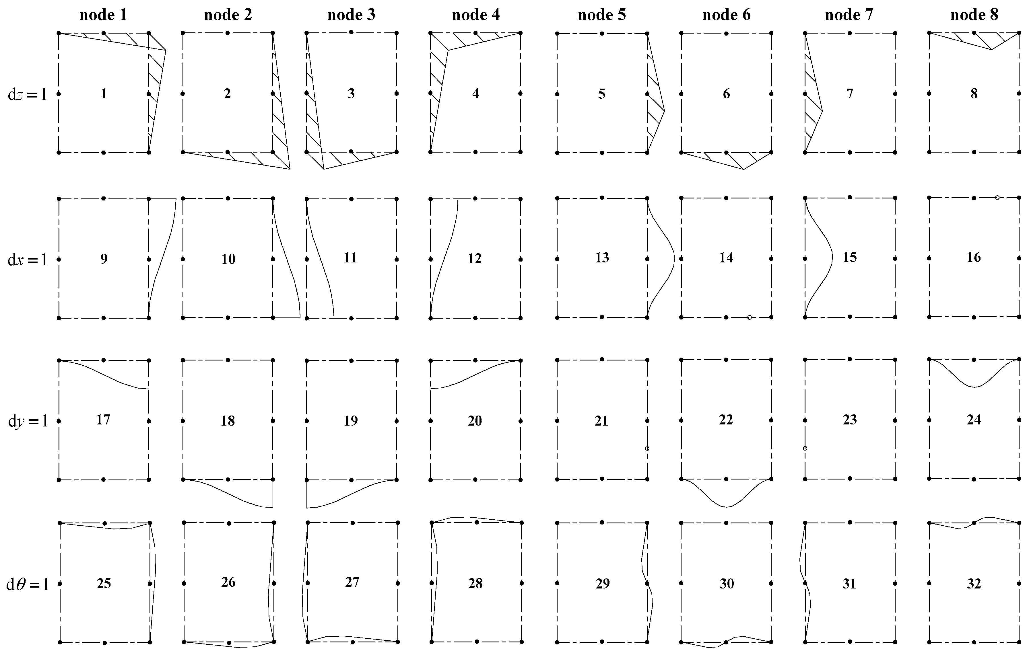
It should be pointed out that the different measures were separately taken for natural and intermediate nodes in the approximation, since they played different roles. For a natural node i, a unit displacement was imposed on it, but null displacements were imposed on all the other natural nodes. The basis functions might have varied within each wall containing node i but were null in all the other walls. For an intermediate node j, the basis function matched the imposition of a unit displacement on node j but matched the null displacements, on all other nodes. This means that the functions varied within the two segments adjacent to node j but were null elsewhere. According to the above guideline, N = 4 × (m_n + m_i) = 32 basis deformation modes were obtained for the cross-section in Figure 2a. As shown in Figure 3, among the thirty-two modes arrayed in a 4 × 8 matrix, each of the 4 rows were derived with an imposed unit displacement on eight nodes, while each of the eight columns represented the deformation modes that resulted from four unit displacements, separately imposed on one node. In the approximation of their deformation shapes, cubic Hermite functions were applied for the normal displacements, and linear functions for the tangential component (the 2rd~4th rows), while the normal displacements were interpolated with the linear Lagrange functions (the first row).

4. Sectional Deformation Modes

The basis deformation modes above were established on the basis of purely kinematic concepts. Though they could serve as basis functions in Equation (2), the problem lied in that their large amount of deformation modes made for a non-reduced model and that the physical interpretation was not intuitive enough to couple with the beam structural behaviors. A set of final deformation modes, which exhibited well-defined structural significance and ranked hierarchically, according to their participations, was very important for a one-dimensional higher-order model. In this section, a procedure to assemble basis deformation modes was developed, similar to the concept of combining like terms in algebra.

This procedure was based on the assumption of considering the cross-section deformation in dynamic systems as the supposition of rigid displacement and elastic deformation of the cross-section, whose amplitudes vary along the longitudinal axis, with a fixed proportion relationship. In this sense, the participation of each basis deformation mode in a final sectional deformation mode can be determined with the data extracted from the modal shapes of certain cross-sections which were derived from the presented model. For convenience, the object cross-section always chose the free end of a cantilevered thin-walled structure, in free vibration. Its slenderness ratio needed to be kept between three and six, since thin-walled structures (Figure 4), in this range, are prone to perform more obvious cross-sectional deformation (see Zhu et al. [30]).

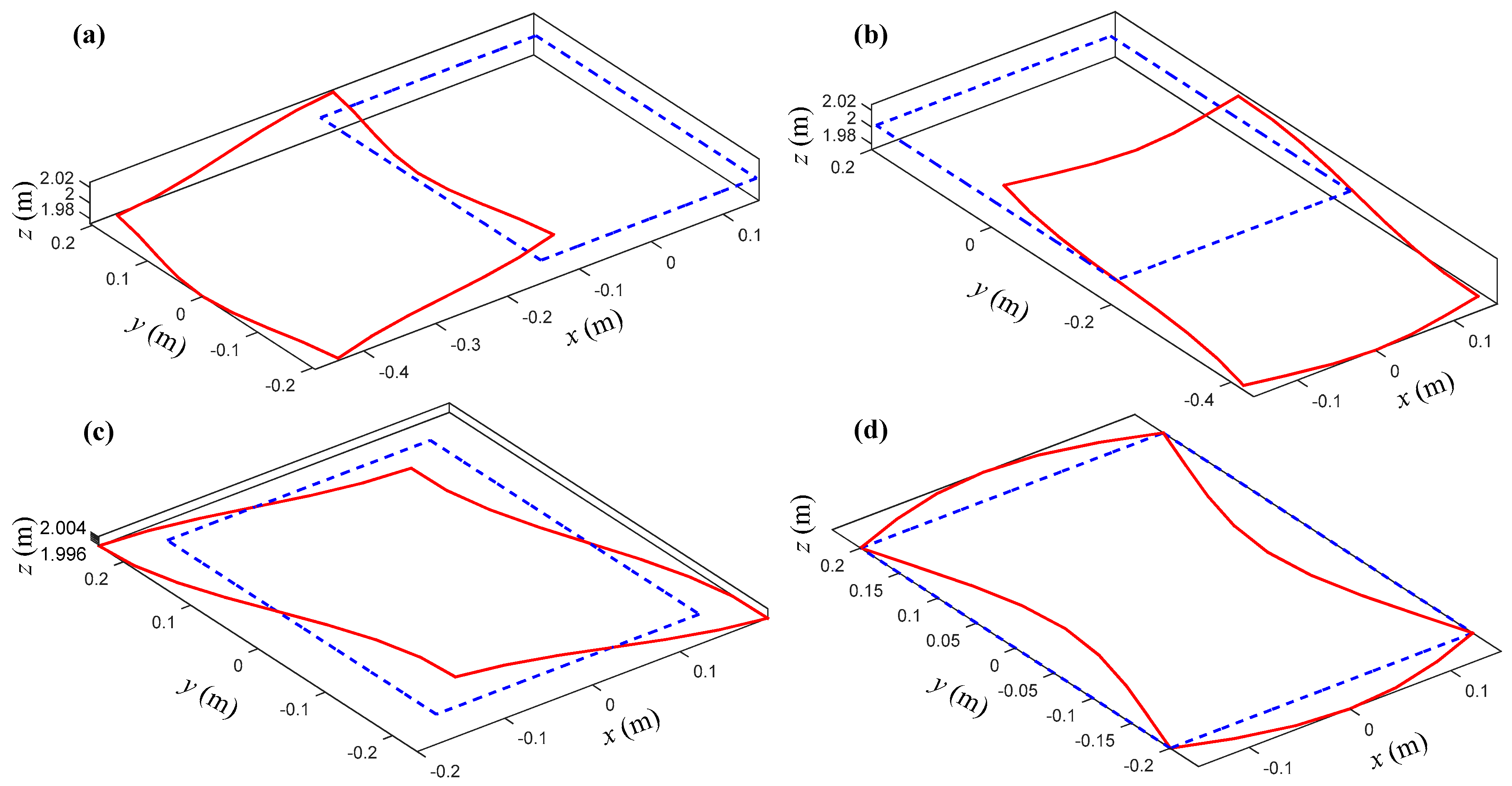
Take the structure in Figure 4 as an example to demonstrate the process. Substituting the set of basis functions shown in Figure 3 into the presented model and employing the boundary conditions in Figure 4, the dynamic model of the thin-walled structure was established for modal analysis. The model was solved in MATLAB with the first few modal shapes extracted and participations of each basis deformation mode obtained for subsequent use. It should be noted that the number of modal shapes to be studied was related to the required number of final deformation modes, which largely influenced the accuracy of the proposed model. In most cases, four to eight modal shapes were essential and might have been enough for thin-walled structures with simple cross-sections. Figure 5 shows the deformed cross-section of the free end for the first 4 modals, where the blue curves indicate an undeformed cross-section and the red ones describe a deformed cross-section. The x and y axes spanned the cross-section plane, while z axis dedicated the cross-section deformation along the longitudinal direction.

For the ease of implementation, basis deformation modes were separated into in-plane and out-of-plane ones, which were to be extracted from the four modal shapes illustrated in Figure 5. In fact, the procedure could be completed to solve the free vibration system, by applying the proposed finite element, since its feature of variable separation, and the amplitudes of each basis deformation mode participating in the modal shapes were obtained simultaneously. Figure 6 demonstrated the amplitudes of basis deformation modes for the first modal of the cantilevered structure.

In Figure 6, the eight amplitudes on the left, corresponded to the out-of-plane mode family, while the twenty-four on the right represented the participations of the in-plane mode family (in accordance with the sequence shown in Figure 3). Here the sign of amplitude value stood for whether the contributing deformation was identical with the predicted positive direction shown in Figure 3. Among each family, a process similar to combining like terms was carried out to linearly superpose basis deformation modes, with equal or opposite amplitudes. For example, among the out-of-plane family with non-null amplitudes in Figure 6, modes 1~4 were like terms (with equal or opposite amplitude values), and so were modes 5 and 7, which were to be assembled together with their amplitudes, as corresponding weights. The assembled modes are designated as primary deformation modes. As shown in Figure 7, two primary deformation modes were obtained through the process. Obviously, the former represented a rigid rotation of the whole cross-section about y-axis. It is a conventional deformation mode in the beam theory of Timoshenko, and here it was numbered as sectional deformation mode I. The other mode was left alone and was numbered as sectional deformation mode V, which represents the first warping deformation (out-of-plane distortion caused by uneven longitudinal extensions, see Carpinteri et al. [31]) of the cross-section. The case confirmed that a modal shape of a thin-walled structure might be a mixture of rigid displacement and elastic deformation of the cross-section.

It should be pointed out that not all primary sectional deformation modes could be identified as final deformation mode. For example, among in-plane mode family demonstrated in Figure 8, modes 1~4 were assembled as a conventional deformation mode representing a rigid translation of the cross-section, being numbered as sectional deformation mode VIII, but not for the rest of the primary deformation modes i, ii and iii (named as secondary deformation modes describing elastic deformation profile of the cross-section). These secondary modes were of no clear physical significance and might not be efficient for a reduced model. For this reason, the three secondary modes were assembled again to form a final distortion mode. This new mode, like the first distortion mode, was associated with rigid translation of the cross-section, along the x-axis and could also be observed in actual experiments. In this sense, it was endued with structural meaning, and numbered as sectional deformation mode XI.

In this way, a total of 14 final sectional deformation modes were identified through the “combining like terms” operation carried out on the first four modal shapes (as shown in Figure 9). Among these modes, modes I, II, III, VIII, IX, and X corresponded to the conventional rigid displacements of the whole cross-section. The other eight modes were newly defined to describe elastic deformation of the cross-section with a minimum total. In general, these new deformation modes were structurally meaningful and linearly independent. Additionally, their arrangements were in accordance with the sequence they appeared in, which showed the capability of a hierarchy.

The proposed simplified approach, although involved with cross-section analysis, was different from both the theory of Camotim et al. [28] for obtaining GBT deformation modes or that of Vieira et al. [29] for formulating the higher order model. Both of these theories have to solve the generalized eigenvalue problem to uncouple the governing differential equations or the basis functions, which is quite demanding. In fact, the authors focused on avoiding this in the process of identifying sectional deformation modes. Instead, a process similar to combining like terms was developed in this paper to assemble basis deformations according to their participations in the constitution of sectional deformation modes. This approach lowered the requirements of mathematical theory and computation load. Additionally, the corresponding process could naturally separate conventional deformation modes from warping and distortion of the cross-section, being propitious to the compatibility with classical beam theories.

5. Illustrative Examples

In order to demonstrate the versatility and clarity of the proposed approach, numerical examples were presented on a cantilevered (Figure 4) thin-walled structure and a fixed–fixed one (with the free end in Figure 4 fixed). It should be noted that in these examples the proposed model was coded and solved in MATLAB [32].

5.1. Convergence Check

Convergence of the proposed finite element was checked with the thin-walled structure shown in Figure 6. As shown in Figure 10, relative errors of the first ten natural frequencies varied with the number of elements employed. Here the converged data were obtained with ninety finite elements. The results showed that a dynamic model with forty elements had converged with relative errors smaller than 0.1%, as compared to those employing ninety elements. Hence, forty elements were essential in the numerical examples.

5.2. Regarding the Cantilevered Structure

To check the validity of the proposed model, numerical examples were carried out on the cantilevered structure in Figure 6.

Table 1. Comparison of the first ten natural frequencies of the cantilevered thin-walled structure.

Mode	Present Model	ANSYS Shell	Relative Error	Warping and Distortion Mode Participations (%)
	fi (Hz)	fAi (Hz)	δi (%)	${\mathit{\chi }}_4$	${\mathit{\chi }}_5$	${\mathit{\chi }}_6$	${\mathit{\chi }}_7$	${\mathit{\chi }}_{11}$	${\mathit{\chi }}_{12}$	${\mathit{\chi }}_{13}$	${\mathit{\chi }}_{14}$
1st	85.201	81.477	4.57	0	0.67	0	0	14.8	0	0	0
2rd	105.45	101.77	3.63	0	0	0.32	0	0	24.0	0	0
3rd	123.40	126.34	−2.33	100	0	0	0	0	0	93.9	0
4th	193.97	190.51	1.82	0	0	0	59.7	0	0	0	100
5th	201.95	202.28	−0.16	0	0	0	85.1	0	0	0	100
6th	217.06	225.57	3.77	0	0	0	73.7	0	0	0	100
7th	237.98	240.80	−1.17	0	3.52	0	0	83.5	0	0	0
8th	263.42	260.68	1.05	0	0	0	65.2	0	0	0	100
9th	283.98	279.35	1.66	0	8.71	0	0	0	95.0	0	0
10th	302.90	307.93	−1.63	0	0	0	67.9	0	0	0	100

showed the information about the first ten modes, including the values of the natural frequencies f_i, obtained with the present model and ANSYS shell theory, the relative differences δ_i and deformation mode participations μ_i. The results of the present model were obtained with forty elements, equally distributed along the beam length. For the ANSYS analysis, the structure was discretized into 1120 Shell 181 4-node elements, distributed as forty elements, along the length, and twenty-eight over the cross-section. The mode participation of each deformation mode was to be calculated by the following.

$${\mu }_i=\{\begin{array}{l}\frac{{\chi }_i{\phi }_{i\max }}{{\displaystyle \sum _{j=1}^{N_1}{\chi }_j{\phi }_{j\max }}}\times 100\%,i=1, 2,\cdots ,N_1\\ \frac{{\chi }_i{\omega }_i}{{\displaystyle \sum _{j=N_1+1}^r{\chi }_j{\omega }_{j\max }}}\times 100\%,i=N_1+1,N_1+2,\cdots ,r\end{array}$$

(20)

where the amplitudes were derived with the values of the free end cross-section, while the relative differences were calculated based on the assumption that the results of ANSYS shell theory were accurate enough.

The results in Table 1 show that the natural frequencies obtained with the present model were very close to those from the ANSYS shell theory. They also proved that warping and distortion modes played important roles in dynamics and large errors might emerge if higher-order modes are ignored. For example, the 3rd~10th modal would not appear when applying conventional beam theories of Timoshenko and Euler-Bernoulli.

The idea could be verified by the results demonstrated in Figure 11 and Figure 12, where non-null amplitudes of final deformation modes have been illustrated to vary along with the longitudinal axis of the structure. Simply put, conventional modes were dominant only in the first two among the first ten modal. It should also be noted that the wave forms were always different between the conventional and the higher-order deformation modes. The phenomenon indicates that in the process of combining like terms, it was unacceptable to superpose primary deformation modes, if they belonged to the rigid displacement and the elastic deformation of the cross-section, respectively. It also showed that warping and distortion were quite independent of conventional modes.

To further study the dynamic behaviors, Figure 13 provides the comparison concerning the 1st~9th modal shapes. The comparison reconfirmed that the present model agreed well with the ANSYS shell theory and also proved that the present model could accurately reproduce three-dimensional behaviors of thin-walled structures. One should bear in mind that here a one-dimensional model was being compared with a three-dimensional finite element model. In many cases, the efficiency and accuracy makes it a qualified alternative to more complicated shell elements. More importantly, the present model could provide results of displacements (even stresses and strains) allowing to identify the decomposition of displacements in terms of the associated deformation modes.

It was also interesting that the sectional deformation modes IV and XIV did not appear together with the conventional modes, which was quite different from other higher-order modes. In this aspect, the two modes were more similar to conventional modes which play important roles in classical beam theory. In consideration of this phenomenon, these modes might be ranked after classical modes but before other higher-order modes, in a follow-up study.

5.3. Regarding the Fixed–Fixed Structure

In the proposed model the set of sectional deformation modes were derived through cross-section analysis of a cantilevered structure. One might consider that if they were a positive natural characteristic of the cross-section, they should be equally applicable in modeling a thin-walled structure with different displacement constraints. To check this, another example was carried out with the structure in Figure 4, with the two ends completely restrained.

Table 2. Comparison of the first six natural frequencies of the fixed–fixed thin-walled structure.

Mode	Present Model	ANSYS Shell	Relative Error
	fi (Hz)	fAi (Hz)	δi (%)
1st	197.00	196.67	0.17
2rd	208.69	216.30	−3.52
3rd	226.88	232.36	−2.36
4th	242.34	249.06	−2.70
5th	276.91	271.31	2.06
6th	294.35	295.06	−0.24

presents the natural frequencies of the first six modes derived from the present model and the ANSYS shell theory, and their relative differences δ_i. Similarly, the results of present model were obtained with forty elements, while the ANSYS analysis was carried out with 1120 Shell 181 4-node elements, distributed as forty elements, along the length, and twenty-eight over the cross-section.

As expected, the results in Table 2 show that the natural frequencies derived from the present model were very close to those from the ANSYS shell theory, with relative differences smaller than 4% for the studied modes. The relative errors exceeded expectation, as they were even smaller than those of a cantilevered thin-walled structure. The reason behind this was worthy of further study.

Besides, Figure 14 provides the comparison concerning the 1st~6th modal shapes, which reconfirmed the good agreement with the ANSYS shell theory. These facts proved that the proposed model, with a set of sectional deformation modes derived from a cantilevered structure, could accurately reproduce three-dimensional behaviors of thin-walled structures with their two ends fixed. Therefore, it is reasonable to deduce that the set of sectional deformation modes are equally applicable to thin-walled structures with different constraints, provided the cross-section is the same. It supports the idea that the set of sectional deformation modes, identified with the present simplified approach, are an inherent property of the thin-walled cross-section. In this sense, the derived model possesses stronger applicability and generality.

6. Conclusions

The study focused on a simplified approach to identify deformation modes of thin-walled structures with prismatic cross-sections. In the course, cross-section discretization was considered to approximate each basis deformation mode with the interpolation of nodal displacements. The structure displacement field was superposed with the derived basis deformation modes and employed in the deduction of the governing differential equation. By means of a modal analysis with the proposed model solved in MATLAB, amplitudes of each basis deformation mode participating in object modal shapes, were obtained and used to assemble final deformation modes with a process similar to combining like terms. The set of final deformation modes were utilized in updating the one-dimensional model as the new basis functions.

The study concludes that the proposed approach is of easy accessibility in theoretical dimension and is of efficiency, in calculation. The set of final deformation modes were of clear physical interpretation and hierarchic capability in forming a reduced model. Especially, numerical examples showed that the developed model has a general application to different constraints and is capable to reproduce three-dimensional behaviors of thin-walled structures. In some cases, the efficiency and accuracy makes it an alternative to shell/plate elements, in commercial finite element software.

References

- Gonçalves, R.; Ritto-Corrêa, M.; Camotim, D. A new approach to the calculation of cross-section deformation modes in the framework of generalized beam theory. Comput. Mech. 2010, 46, 759–781. [Google Scholar] [CrossRef]
- Yu, W.; Hodges, D.H. Generalized Timoshenko theory of the variational asymptotic beam sectional analysis. J. Am. Helicopter Soc. 2005, 50, 46–55. [Google Scholar] [CrossRef]
- Harursampath, D.; Harish, A.B.; Hodges, D.H. Model reduction in thin-walled open-section composite beams using variational asymptotic method. Part I: Theory Thin-Walled Struct. 2017, 117, 356–366. [Google Scholar]
- Carrera, E.; Pagani, A.; Banerjee, J.R. Linearized buckling analysis of isotropic and composite beam-columns by Carrera Unified Formulation and dynamic stiffness method. Mech. Adv. Mater. Struct. 2016, 23, 1092–1103. [Google Scholar] [CrossRef]
- Yan, Y.; Pagani, A.; Carrera, E. Exact solutions for free vibration analysis of laminated, box and sandwich beams by refined layer-wise theory. Compos. Struct. 2017, 175, 28–45. [Google Scholar] [CrossRef]
- Brillante, C.; Morandini, M.; Mantegazza, P. Characterization of beam stiffness matrix with embedded piezoelectric devices via generalized eigenvectors. Int. J. Solids Struct. 2015, 59, 37–45. [Google Scholar] [CrossRef]
- Naccache, F.; El Fatmi, R. Buckling analysis of homogeneous or composite I-beams using a 1D refined beam theory built on Saint Venant’s solution. Thin-Walled Struct. 2018, 127, 822–831. [Google Scholar] [CrossRef]
- Vlasov, V.Z. Thin-Walled Elastic Beams; Israel Program for Scientific Translations: Jerusalem, Israel, 1961. [Google Scholar]
- Umansky, A.A. Torsion and Bending of Thin-Walled Aircraft Structures; Oboronghiz: Moscow, Russia, 1939. [Google Scholar]
- Kim, Y.Y.; Kim, J.H. Thin-walled closed box beam element for static and dynamic analysis. Int. J. Numer. Methods Eng. 2015, 45, 473–490. [Google Scholar] [CrossRef]
- Kovvali, R.K.; Hodges, D.H.; Yu, W.; Kim, H.S.; Kim, J.S. Comments on “A Rankine-Timonshenko-Vlasov beam theory for anisotropic beams via an asymptotic strain energy transformation”. Eur. J. Mech.-A/Solids 2016, 60, 359–360. [Google Scholar] [CrossRef]
- Gonçalves, R.; Peres, N.; Bebiano, R.; Camotim, D. Global–Local-Distortional Vibration of Thin-Walled Rectangular Multi-Cell Beams. Int. J. Struct. Stab. Dyn. 2015, 15, 1540022. [Google Scholar] [CrossRef]
- Chen, S.S.; Tian, Z.L.; Gui, S.R. Shear lag effect of a single-box multi-cell girder with corrugated steel webs. J. Highw. Transp. Res. Dev. (Engl. Ed.) 2016, 10, 33–40. [Google Scholar] [CrossRef]
- Lacidogna, G. Tall buildings: Secondary effects on the structural behaviour. Proc. Inst. Civ. Eng.-Struct. Build. 2017, 170, 391–405. [Google Scholar] [CrossRef]
- Seguy, S.; Campa, F.J.; Lopez de Lacalle, L.N.; Arnaud, L.; Dessein, G.; Aramendi, G. Toolpath dependent stability lobes for the milling of thin-walled parts. Int. J. Mach. Machinab. Mater. 2008, 4, 377–392. [Google Scholar] [CrossRef]
- de Lacalle, L.N.L.; Viadero, F.; Hernández, J.M. Applications of dynamic measurements to structural reliability updating. Probab. Eng. Mech. 1996, 11, 97–105. [Google Scholar] [CrossRef]
- Vieira, R.F.; Virtuoso, F.B.E.; Pereira, E.B.R. A higher order thin-walled beam model including warping and shear modes. Int. J. Mech. Sci. 2013, 66, 67–82. [Google Scholar] [CrossRef]
- Pagani, A.; Boscolo, M.; Banerjee, J.R.; Carrera, E. Exact dynamic stiffness elements based on one-dimensional higher-order theories for free vibration analysis of solid and thin-walled structures. J. Sound Vib. 2013, 332, 6104–6127. [Google Scholar] [CrossRef] [Green Version]
- Schardt, R. Generalized beam theory—An adequate method for coupled stability problems. Thin-Walled Struct. 1994, 19, 161–180. [Google Scholar] [CrossRef]
- Gonçalves, R.; Bebiano, R.; Camotim, D. On the shear deformation modes in the framework of generalized beam theory. Thin-Walled Struct. 2014, 84, 325–334. [Google Scholar] [CrossRef]
- de Miranda, S.; Madeo, A.; Melchionda, D.; Patruno, L.; Ruggerini, A.W. A corotational based geometrically nonlinear Generalized Beam Theory: Buckling FE analysis. Int. J. Solids Struct. 2017, 121, 212–227. [Google Scholar] [CrossRef]
- Mohammad-Abadi, M.; Daneshmehr, A.R. Modified couple stress theory applied to dynamic analysis of composite laminated beams by considering different beam theories. Int. J. Eng. Sci. 2015, 87, 83–102. [Google Scholar] [CrossRef]
- Gonçalves, R.; Camotim, D. GBT deformation modes for curved thin-walled cross-sections based on a mid-line polygonal approximation. Thin-Walled Struct. 2016, 103, 231–243. [Google Scholar] [CrossRef]
- Garcea, G.; Gonçalves, R.; Bilotta, A.; Manta, D.; Bebiano, R.; Leonetti, L.; Magisano, D.; Camotim, D. Deformation modes of thin-walled members: A comparison between the method of Generalized Eigenvectors and Generalized Beam Theory. Thin-Walled Struct. 2016, 100, 192–212. [Google Scholar] [CrossRef]
- Genoese, A.; Genoese, A.; Bilotta, A.; Garcea, G. A generalized model for heterogeneous and anisotropic beams including section distortions. Thin-Walled Struct. 2014, 74, 85–103. [Google Scholar] [CrossRef]
- Vieira, R.F.; Virtuoso, F.B.E.; Pereira, E.B.R. A higher order beam model for thin-walled structures with in-plane rigid cross-sections. Eng. Struct. 2015, 84, 1–18. [Google Scholar] [CrossRef]
- Vieira, R.F.; Virtuoso, F.B.E.; Pereira, E.B.R. Definition of warping modes within the context of a higher order thin-walled beam model. Comput. Struct. 2015, 147, 68–78. [Google Scholar] [CrossRef]
- Bebiano, R.; Gonçalves, R.; Camotim, D. A cross-section analysis procedure to rationalise and automate the performance of GBT-based structural analyses. Thin-Walled Struct. 2015, 92, 29–47. [Google Scholar] [CrossRef]
- Vieira, R.F.; Virtuoso, F.B.; Pereira, E.B.R. A higher order model for thin-walled structures with deformable cross-sections. Int. J. Solids Struct. 2014, 51, 575–598. [Google Scholar] [CrossRef]
- Zhu, Z.; Zhang, L.; Shen, G.; Cao, G. A one-dimensional higher-order theory with cubic distortional modes for static and dynamic analyses of thin-walled structures with rectangular hollow sections. Acta Mech. 2016, 227, 2451–2475. [Google Scholar] [CrossRef]
- Carpinteri, A.; Lacidogna, G.; Nitti, G. Open and closed shear-walls in high-rise structural systems: Static and dynamic analysis. Curved Layer. Struct. 2016, 3, 154–171. [Google Scholar] [CrossRef]
- Hunt, B.R.; Lipsman, R.L.; Rosenberg, J.M. A Guide to MATLAB: For Beginners and Experienced Users; Cambridge University Press: Cambridge, UK, 2014. [Google Scholar]
Figure 1.
Global (x, y, z) and local (s, n, z) coordinate systems of a thin-walled structure with a branched cross-section profile.
Figure 2.
Discretization of a prismatic thin-walled cross-section: (a) A rectangular hollow cross-section; (b) a branched hollow cross-section.
Figure 3.
Basis deformation modes of a thin-walled, rectangular, hollow cross-section with eight discretization nodes.
Figure 4.
A cantilevered thin-walled structure with geometry and material parameters as shown for modal analyses.
Figure 5.
Deformed cross-sections of the free end for the first four modal shapes of the thin-walled structure with a rectangular hollow cross-section: (a) The 1st modal, (b) the 2rd modal, (c) the 3rd modal, and (d) the 4th modal.
Figure 6.
Amplitudes of basis deformation modes participating in the first modal of the free end cross-section of a cantilevered thin-walled structure.
Figure 7.
Assemblage of out-of-plane mode family for the first modal of a thin-walled structure with a rectangular hollow cross-section.
Figure 8.
Assemblage of in-plane mode family for the first modal of a thin-walled structure with a rectangular hollow cross-section.
Figure 9.
Sectional deformation modes identified from the first 4 modal shapes of the cantilevered thin-walled structure with a rectangular hollow cross-section.
Figure 10.
Convergence of the first ten natural frequencies of the cantilevered thin-walled structure, varying with the number of employed finite elements.
Figure 11.
Longitudinal variations of the out-of-plane generalized displacements of the thin-walled structures, in free vibration analysis.
Figure 12.
Longitudinal variations of the in-plane generalized displacements of the thin-walled members, in free vibration analysis.
Figure 13.
Comparison of modal shapes of the cantilevered thin-walled structure between ANSYS shell model (the right) and present model (the left).
Figure 14.
Comparison of the modal shapes of the fixed–fixed thin-walled structures, between the ANSYS shell model (the right) and the present model (the left).