Information-Bottleneck Decoding of High-Rate Irregular LDPC Codes for Optical Communication Using Message Alignment

Abstract

In high-throughput applications, low-complexity and low-latency channel decoders are inevitable. Hence, for low-density parity-check (LDPC) codes, message passing decoding has to be implemented with coarse quantization—that is, the exchanged beliefs are quantized with a small number of bits. This can result in a significant performance degradation with respect to decoding with high-precision messages. Recently, so-called information-bottleneck decoders were proposed which leverage a machine learning framework (i.e., the information bottleneck method) to design coarse-precision decoders with error-correction performance close to high-precision belief-propagation decoding. In these decoders, all conventional arithmetic operations are replaced by look-up operations. Irregular LDPC codes for next-generation fiber optical communication systems are characterized by high code rates and large maximum node degrees. Consequently, the implementation complexity is mainly influenced by the memory required to store the look-up tables. In this paper, we show that the complexity of information-bottleneck decoders remains manageable for irregular LDPC codes if our proposed construction approach is deployed. Furthermore, we reveal that in order to design information bottleneck decoders for arbitrary degree distributions, an intermediate construction step which we call message alignment has to be included. Exemplary numerical simulations show that incorporating message alignment in the construction yields a 4-bit information bottleneck decoder which performs only $0.15$ dB worse than a double-precision belief propagation decoder and outperforms a min-sum decoder.

1. Introduction

It is well-known that the decoding of channel codes is one of the major bottlenecks in baseband signal processing. To realize next-generation fiber-optical systems with bit rates of 400 $\mathrm{Gbit}/\mathrm{s}$ and above, high-speed decoding algorithms are inevitable. A very powerful and well-known class of error-correcting codes are the so-called low-density parity-check (LDPC) codes [1]. The design of LDPC codes for optical communications has been discussed in recent works [2,3,4,5,6,7]. In contrast to wireless communication, the coding schemes in optical communication use comparably high code rates $R>0.8$ to keep the redundancy at a minimum. Furthermore, bit error rates of ${10}^{-15}$ are required in optical communication systems, which is often challenging to achieve with LDPC codes due to their characteristic error floor. Nevertheless, recent works [2,3,4,5,6,7] underlined the potential of LDPC codes as promising candidates in future optical communication systems. For a detailed summary of coding schemes for optical systems, we refer the interested reader to [7,8].

LDPC codes fully unfold their capacity-approaching error-correction capabilities under message passing decoding only if precise and computationally complex belief propagation decoding is performed. The high computational complexity is mainly induced by two properties of message passing decoding: On the one hand, to reliably exchange soft information and thus ensure optimum performance, the exchanged messages have to be represented precisely. On the other hand, elaborate arithmetic operations which combine incoming beliefs (e.g., at a check node) form a major performance bottleneck. The computational burden of high-precision message passing decoding diminishes the achievable throughput and latency and requires impractically complex implementations. Instead, practical hardware implementations use finite-precision message passing algorithms where the messages are quantized and the node operations are simplified by smart approximations. However, the error-rate performance of such finite-precision decoders deteriorates significantly with decreasing precision [9].

Recently, a fundamentally different approach was proposed: the so-called information bottleneck or look-up table decoder [9,10,11,12,13,14]. This decoder leverages ideas from information theory and machine learning and differs from conventional finite-precision decoders mainly in the following two points:

• Instead of executing the conventional arithmetic exactly or approximated in the nodes with discrete values, the node operations are replaced by relevant-information-maximizing look-up tables which map discrete input messages onto discrete output messages. The required message mappings are designed using a relevant-information-preserving clustering technique, such as the information bottleneck method as shown in [10,11] or using similar algorithms [12,14].
• The relevant-information-maximizing look-up tables let messages that are log-likelihood ratios (LLRs) become obsolete. Instead, integer-valued pointers to look-up table entries, sometimes called cluster indices, are exchanged, which do not represent LLRs.

In our previous works, we have already shown that four bits are sufficient to represent the exchanged messages [10,11,15]: our proposed 4-bit information bottleneck decoder for regular LDPC codes approaches the performance of double precision belief-propagation decoding up to $0.1$ dB over $E_b/N_0$ with a vastly reduced implementation complexity [11]. Recently published investigations of FPGA implementations of similarly designed look-up table-based decoders in [16] showed that look-up table decoders for regular codes can achieve a throughput of 588 $\mathrm{Gbit}/\mathrm{s}$ and are superior to conventional decoding techniques in terms of energy efficiency and area efficiency.

However, the existing work is mainly limited to regular LDPC codes. A first step towards information bottleneck decoders for irregular LDPC codes was described in [9], where the authors advocate that existing LDPC codes are often ill-suited to information-bottleneck decoding and thus proposed a joint optimization of the node-degree distribution and the look-up tables. That is, they proposed to adapt the code to the specific shortcomings of the available information bottleneck decoding method instead of fundamentally changing the decoder design.

In contrast, in [17] we devised a generalized design approach suitable for arbitrary irregular LDPC codes as defined in many standards (e.g., IEEE 802.11 or DVB-S2) without any modification of the LDPC code itself. We proposed an intermediate processing step called message alignment which we first applied in the context of information-bottleneck channel quantizers for higher-order modulation schemes [18] and distributed information-bottleneck sensor design [19].

Caused by the high coding rate required in optical communication systems, respective LDPC codes incorporate very high node degrees. In this paper, we show that existing construction techniques cause an undesirable growth in memory demand when they are applied to high rate codes, due to a large number of look-up tables.

In detail, this paper contains the following main contributions:

• We extend the decoder construction framework from [13,19] to be applicable to arbitrary irregular LDPC codes also with high code rates.
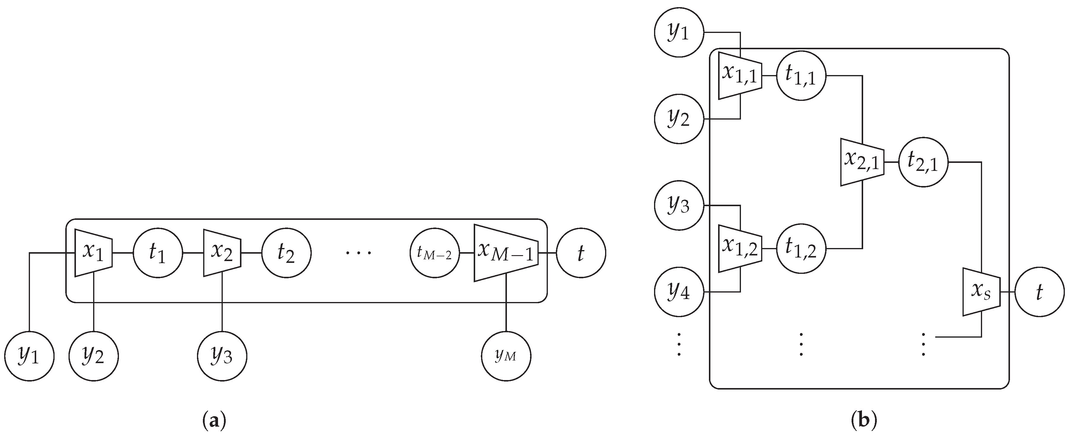
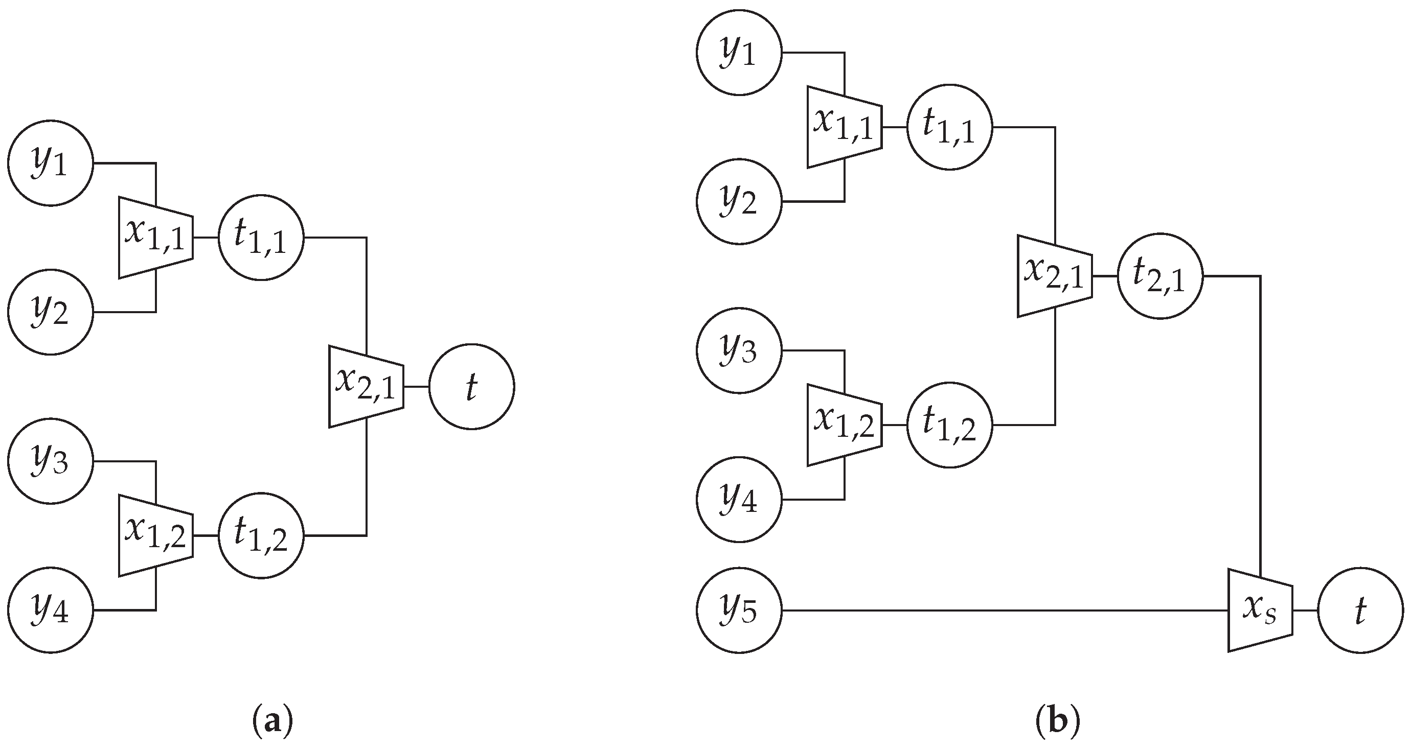
• We introduce a novel tree-like look-up pattern. With this strategy, the relation between the number of look-ups required per iteration and node degree changes from linear to logarithmic.
• We derive the underlying information-theoretic problem formulation and explain how the intermediate optimization technique called message alignment can be incorporated.
• We construct a 4-bit information bottleneck decoder for irregular LDPC codes with a code rate $R=0.8$, where all conventional arithmetic in the nodes is replaced by simple look-up tables and only 4-bit integer-valued messages are passed.
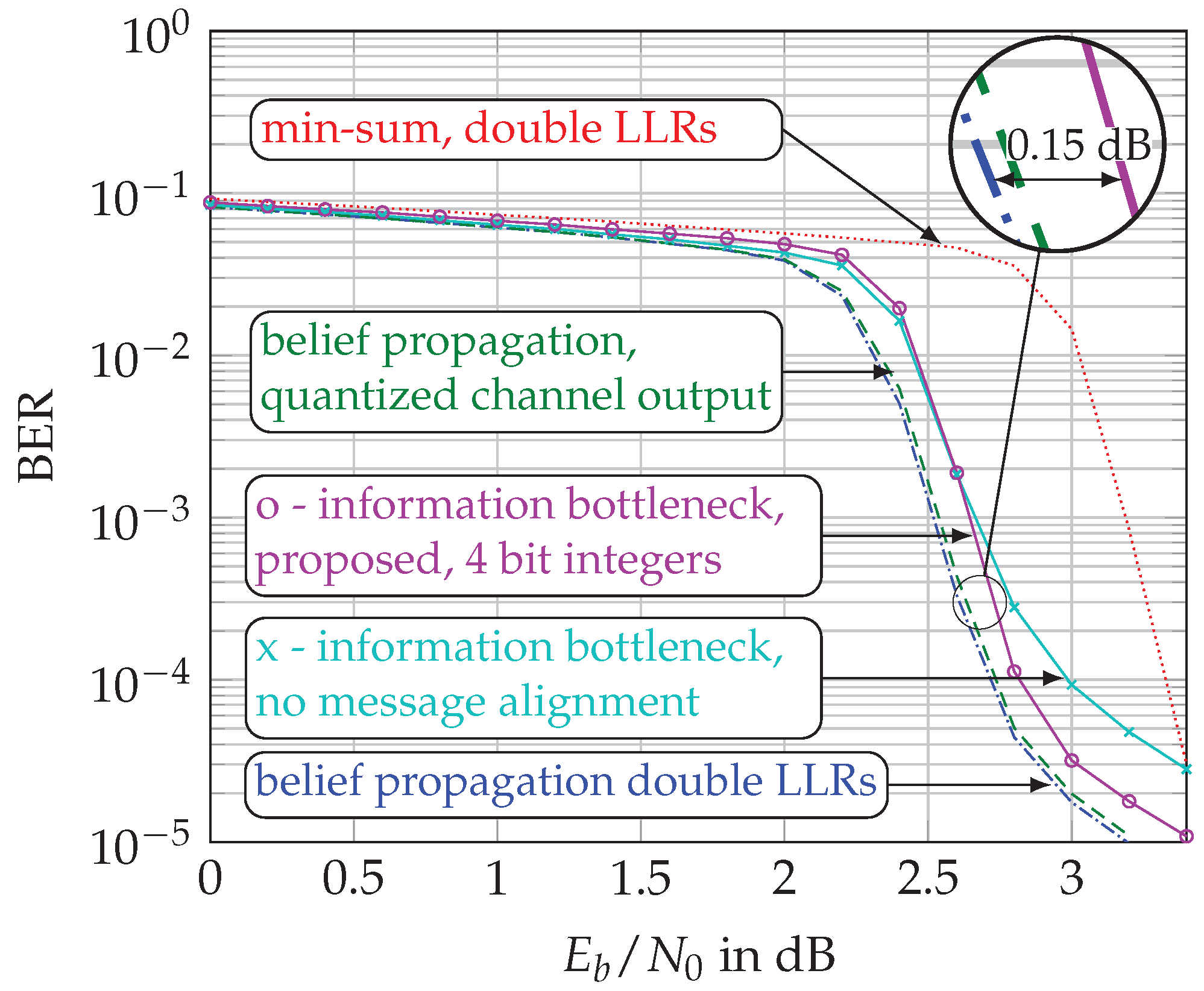
• Our proposed decoder achieves error-rates superior to min-sum decoding and only $0.15$ dB away from double-precision belief propagation decoding.

The paper is organized as follows. The information bottleneck method and LDPC codes are briefly reviewed in Section 2. In Section 3, we propose message alignment, resulting in a general information bottleneck decoder design approach for arbitrary irregular LDPC codes. In Section 4 we provide detailed insights concerning the internal structure of the look-up tables replacing the arithmetic operations. Based on these considerations, a more efficient design strategy is proposed. In Section 5, numerical simulations comparing the performance of our proposed decoder with several reference systems are provided. Section 6 concludes the paper.

2. Prerequisites

This section briefly reviews LDPC codes and the information bottleneck method. Throughout the paper, we use the following notation: the elements $y\in \mathcal{Y}$ from the event space of a discrete random variable Y occur with probability $\mathrm{Pr}(Y=y)$, and $p\left(y\right)$ defines the corresponding probability distribution. The cardinality or alphabet size of the random variable Y is denoted by $\left|\mathcal{Y}\right|$. The joint distribution of X and Y is denoted $p(x,y)$.

2.1. Low-Density Parity-Check (LDPC) Codes

An LDPC code is defined by a sparse $N_c\times N_v$ parity check matrix $\mathbf{H}$. To analyze the structure of $\mathbf{H}$, an LDPC code can be visualized using a Tanner graph. A Tanner graph is a bipartite graph consisting of one set for the $N_v$ variable nodes and the other set for the $N_c$ check nodes. This is schematically illustrated in Figure 1. Irregular LDPC codes are typically described using their ensemble characteristics, and therefore, the connections between the two sets are characterized probabilistically by the edge-degree distributions for the variable nodes and the check nodes [20]:

$$\lambda \left(z\right)=\sum _{d=2}^{{\lambda }_{\max }}{\lambda }_d{z}^{d-1},\rho \left(z\right)=\sum _{d=2}^{{\rho }_{\max }}{\rho }_d{z}^{d-1},$$

(1)

where ${\lambda }_d$ denotes the fraction of edges connected to variable nodes with degree d and ${\rho }_d$ denotes the fraction of edges connected to check nodes with degree d. The LDPC code is called regular if all variable nodes have the same degree $d_v$ and all check nodes have the same degree $d_c$, and otherwise the LDPC code is called irregular. The general derivations in the next sections hold for both node types (i.e., variable nodes and check nodes). Thus, we formally introduce a general edge-degree distribution

$$\omega \left(z\right)=\sum _{d=2}^{{\omega }_{\max }}{\omega }_d{z}^{d-1}$$

(2)

to indicate when the derived equations are applicable for any node type.

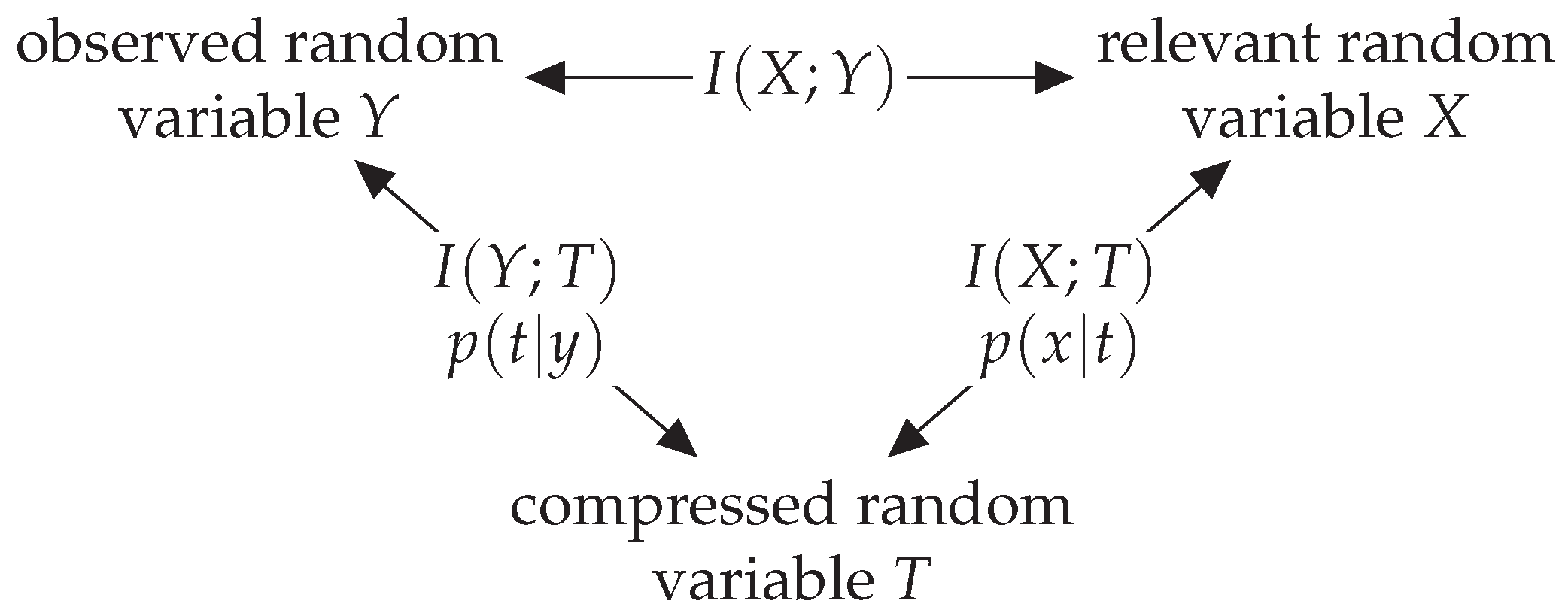
2.2. The Information Bottleneck Method

The information bottleneck method is a generic unsupervised clustering framework from the field of machine learning [21,22]. The so-called information bottleneck setup is visualized in Figure 2. Having defined a random variable X termed the relevant random variable, the principal aim of the information bottleneck method is to extract all relevant information contained in an observation Y, by squeezing Y through a compact bottleneck represented by the compression variable T. More precisely, the information bottleneck method attempts to design a compression mapping $p\left(t\right|y)$ which maps an observation Y onto a compact compression variable T.

Typically, $\left|\mathcal{Y}\right|\gg \left|\mathcal{T}\right|$. The key idea is to design $p\left(t\right|y)$ such that the maximum possible amount of mutual information $\mathrm{I}(T;X)\le \mathrm{I}(X;Y)$ is preserved under a constraint for the cardinality $\left|\mathcal{T}\right|$. Several information bottleneck algorithms exist, intended to find a locally-optimum compression mapping $p\left(t\right|y)$ [22]. All information bottleneck algorithms input a joint distribution $p(x,y)$ and yield the compression mapping $p\left(t\right|y)$ and a joint distribution $p(x,t)=p\left(x\right|t\left)p\right(t)$. Typically, in the context of signal processing, one assumes a deterministic input–output mapping (e.g., at a quantizer). Hence, it is often sufficient to consider only deterministic mappings $p\left(t\right|y)$ (i.e., $p\left(t\right|y)\in \{0,1\}\forall (t,y)$). Such mappings can be interpreted as look-up tables mapping y onto t. More details related to the information bottleneck method can be found in [21,22]. Throughout the paper, we use the terms mapping and clustering synonymously. A more detailed overview and comparison of information bottleneck algorithms can be found in [22,23]. Please note that when performing a mapping $p\left(t\right|y)$, any physical meaning contained in Y is lost (i.e., the compression variable T on its own has no distinct meaning and the event space $\mathcal{T}$ can be chosen arbitrarily). Hence, a coupling between the relevant variable X and T is needed, given by $p\left(x\right|t)$. We sometimes refer to this distribution as the meaning of a cluster index t with respect to x.

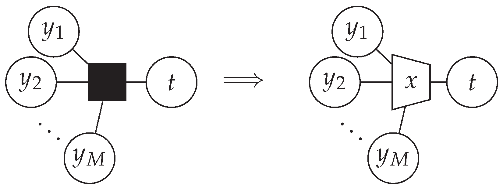
2.3. Information-Bottleneck Signal Processing and Information Bottleneck Graphs

Despite having its origin in machine learning and numerous classification problems, the information bottleneck has recently been used to design various communication systems. Application fields pairing the information bottleneck and signal processing include LDPC decoding, channel estimation, relaying, C-RAN, polar code construction, sensor networks, etc. [10,18,19,24,25,26]. Leveraging information theoretical concepts to design practical systems is termed information-bottleneck signal processing [15]. Information-bottleneck signal processing using the information bottleneck method differs from conventional approaches in mainly three points. The first fundamental difference is the focus on the preservation of the so-called relevant information as a distortion measure in contrast to conventional measures like the Euclidean distance or the mean-squared error. As a result, it is possible to obtain compact but very informative representations of the processed samples. In a second step, these compression mappings or clusterings replace the actual arithmetic operations. Thus, in addition to a reduction of memory due to the compression, the computational complexity is also reduced by replacing arithmetic operations with look-up operations. Finally, information-bottleneck signal processing is a system-oriented design technique rather than a function-oriented technique. That is, instead of finding local approximations of certain functions, the overall aim of information-bottleneck signal processing is to optimize the flow of relevant information in the system from the data aggregation to the decision unit. For a more detailed review of information-bottleneck signal processing, we refer the reader to [15].

Due to the system-oriented design, finding the most efficient structure which optimizes the flow of relevant information can be quite cumbersome [15]. Therefore, information bottleneck graphs were introduced in [27] which extend factor graphs [28] by a compact description of the flow of relevant information to provide a vivid graphical representation of the system. Information bottleneck graphs indicate where the use of information-bottleneck clusterings is beneficial, and thus help to simplify the design [27]. For this purpose, a modified node symbol is used for all factor nodes representing compression mappings $p\left(t\right|y)$ that were designed using the information bottleneck method. In an information bottleneck graph, the typical square notation of factor nodes is replaced by a trapezoid symbol for all compression mappings. An example is shown in Figure 3. The relevant variable labels are written in the center of the trapezoid symbol to illustrate the information bottleneck with respect to this variable. The compression variable is connected to the shortest side of the trapezoid. All other connected variables correspond to a (possibly multivariate) observed variable. The example in Figure 3 illustrates the flow of relevant information on x from random vector $\mathbf{y}={[y_1,\dots ,y_M]}^{\mathrm{T}}$ to t. That is, $t=f\left(\mathbf{y}\right)$ compresses $\mathbf{y}$ while preserving relevant information on x.

3. Information Bottleneck Decoders for Irregular LDPC Codes Using Message Alignment

This section contains our main contributions. After a brief review of information bottleneck decoder design for regular LDPC codes, we generalize this concept to arbitrary irregular LDPC codes. First, we derive the relevant-information-preserving message mappings, which replace the conventional arithmetic operations. Then, we present two perspectives, a graphical and an information-theoretical one, to motivate the need for an additional step in the decoder design. As a result, we propose a technique that we call message alignment.

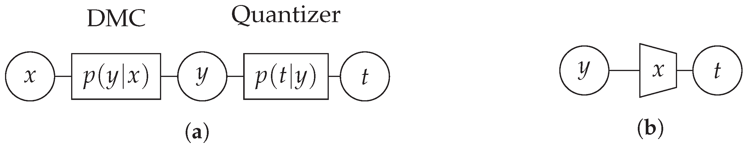
3.1. Information-Bottleneck Channel Quantizer for Arbitrary Discrete Memoryless Channels

In every digital communication system, the received, possibly continuous channel output y is fed into an analog-to-digital converter to obtain discrete-valued receive samples (cf. Figure 4a). In theoretical considerations, the effect of the quantizer is often ignored. This assumption is only valid if the resolution of the quantizer is very high. When transmitting at very high speed, the quantizer marks the first bottleneck in the receiver chain: coarse quantization of only a few bits is required for high-throughput implementations. In the context of information-bottleneck signal processing, the quantizer is the first unit in the receiver which can be optimized using the information bottleneck method. Figure 4b depicts the respective information bottleneck graph. As mentioned in the previous section, the information bottleneck method requires the joint distribution $p(x,y)$ of the relevant random variable X and the observed random variable Y. In general, an assumed channel model implies the transition probabilities described by $p\left(y\right|x)$. The transition model $p\left(y\right|x)$ multiplied by the prior distribution $p\left(x\right)$ of the channel input yields the joint distribution $p(x,y)$. In the case of a channel output quantizer, an information bottleneck algorithm which delivers a deterministic mapping $p\left(t\right|y)$ is a natural choice. If designed using the information bottleneck, the quantization regions of an information-bottleneck channel quantizer are only described by a cluster index t, instead of a cluster representative which has to be represented with high resolution. These cluster indices, which are typically integers, are forwarded to subsequent units (e.g., for the channel decoder that is introduced in the next subsection). Information-bottleneck channel quantizers can also be generalized to support higher-order modulation schemes which require a de-mapper before the channel decoder [18].

3.2. Information Bottleneck Decoders for Regular LDPC Codes

As mentioned in the Introduction, the need for quasi-continuous LLRs and computationally complex node operations makes belief propagation decoding challenging. Information bottleneck decoders have been shown to overcome this impairment. That is, they pair low implementation complexity and near-optimal performance [10,12,13]. The fundamental idea of these decoders is to propagate compressed but highly informative integer-valued messages along the edges of a Tanner graph. In a second step, node operations optimized for discrete input alphabets are designed. These operations are look-up operations mapping a set of discrete incoming messages onto a discrete outgoing message, thereby neglecting the original arithmetic operations. The vital task of this mapping is to ensure that as much relevant information as possible gained by the processing of the incoming messages is contained in the compactly represented output. A suitable information-theoretic framework for such problems is the information bottleneck method [21].

The information bottleneck method constructs relevant-information-maximizing clusterings given a joint probability distribution of the observed random variable Y and relevant random variable X. In the context of LDPC decoder design, the observed random variables are the M incoming discrete messages $\mathbf{y}={[y_1,\cdots ,y_M]}^{\mathrm{T}}$, and the relevant random variable X is a codeword bit. For a variable node, X represents the underlying code bit $b_i$ of a particular node, whereas if the mapping is designed for a check node, X represents the (mod 2)-sum of the connected code bits $b_1,\cdots ,b_M$ (cf. Figure 1). The joint distribution $p(x,\mathbf{y})$ serving as input for the information bottleneck algorithms is determined using discrete density evolution [13]. Although classical density evolution was originally intended to find the decoding thresholds of an LDPC code ensemble, previous works have shown that the joint distributions exchanged in discrete density evolution equal exactly the necessary input distributions for the information bottleneck method [10,11,12,13]. The term discrete in discrete density evolution implies that instead of processing continuous joint distributions, the event space of the observed random variable Y (i.e., $\mathcal{Y}=\{0,1,\cdots ,|\mathcal{Y}|-1\}$) is also discrete, meaning that the realizations y are from a finite alphabet with cardinality $\left|\mathcal{Y}\right|$. Hence, given an observation vector $\mathbf{y}$, ${\left|\mathcal{Y}\right|}^M$ possible input combinations exist. To prevent an exponential growth in the number of input combinations while passing $p(x,\mathbf{y})$ over the Tanner graph during discrete density evolution, $p(x,\mathbf{y})$ is squeezed through a compact information bottleneck. That is, a relevant-information preserving clustering $p\left(t\right|\mathbf{y})$ is introduced such that the outgoing message $t\in \mathcal{T}=\{0,1,\cdots ,|\mathcal{T}|-1\}$ is from a finite alphabet with cardinality $\left|\mathcal{T}\right|\ll {\left|\mathcal{Y}\right|}^M$. Once this clustering is found, the actual decoding simplifies to simple look-ups in offline generated tables, which map the sequence of incoming integers $\mathbf{y}$ onto an outgoing integer-valued message t. For a more mathematical analysis and a detailed description of information bottleneck decoders for regular codes, we refer the reader to [10,11,12,13].

3.3. Relevant-Information-Preserving Clusterings for Arbitrary Irregular LDPC Codes

In contrast to regular LDPC codes, irregular LDPC codes are characterized by nodes with various degrees (i.e., the number of incoming messages differs). Thus, the input joint distribution $p_d(x,\mathbf{y})$ for the information bottleneck depends on the node degree d. Consequently, it is not sufficient to design message mappings only for each node type, but for each node type considering the individual node degrees. For ease of notation, we introduce subscripts for the distributions indicating the node degree. That is, $p_d\left(t\right|\mathbf{y})$ is the relevant-information-preserving clustering at a node with degree d found given the input joint distribution $p_d(x,\mathbf{y})$. In density evolution, a code ensemble is considered. That is, instead of a particular irregular LDPC code with a certain parity-check matrix, the connectivity between variable and check nodes is only known on average defined by the degree distribution. To construct the required input joint distributions $p_d(x,\mathbf{y})$, discrete density evolution from [13] needs to be extended to consider the degree distribution of the code ensemble.

Conventional density evolution is a technique to analyze the error correction performance of the code ensemble. In the conventional density evolution scheme for irregular codes, one tracks the average output distributions $p_{\overline{d}}(x,\mathbf{y})$ of the variable and the check nodes. Therefore, the actual output distribution $p_d(x,\mathbf{y})$ for each node degree d is weighted according to the edge-degree distributions. That is,

$$p_{\overline{d}}(x,\mathbf{y})=\sum _{d=2}^{{\omega }_{\max }}{\omega }_d{p}_d(x,\mathbf{y}),$$

(3)

where ${\omega }_d$ is from the edge-degree distribution [20].

In discrete density evolution, a relevant-information-preserving clustering is crucial to inhibit the exponential growth of the possible input combinations. Thus, $p_{\overline{d}}(x,t)$ instead of $p_{\overline{d}}(x,\mathbf{y})$ has to be tracked in discrete density evolution. We define the average distribution $p_{\overline{d}}(x,t)$ as

$$p_{\overline{d}}(x,t)=\sum _{d=2}^{{\omega }_{\max }}{\omega }_d{p}_d(x,t)=\sum _{d=2}^{{\omega }_{\max }}{\omega }_d\sum _{\mathbf{y}\in {\mathcal{Y}}_d^{\mathrm{vec}}}{p}_d\left(t\right|\mathbf{y})p_d(x,\mathbf{y}),$$

(4)

where ${\mathcal{Y}}_d^{\mathrm{vec}}$ denotes the set of all possible combinations of $\mathbf{y}$ for a node with degree d.

Please note that, assuming a trivial straightforward generalization of information bottleneck decoders to irregular LDPC codes, one would stop at this point. In this case, look-ups in node-degree-specific tables $p_d\left(t\right|\mathbf{y})$ would replace the node operations, and only integer values cluster indices would be exchanged. However, in the next subsections, we demonstrate that such a design approach is not beneficial. Given these findings, we propose to include an additional integral step in the construction process.

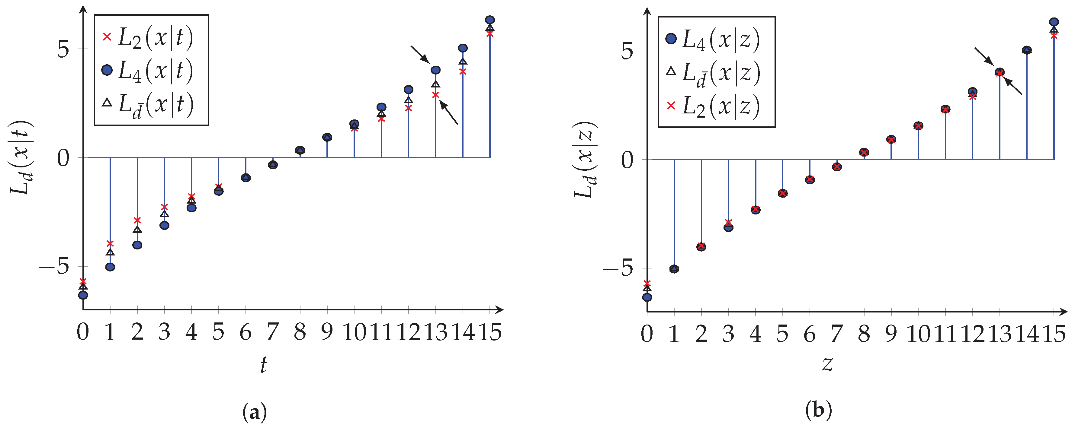
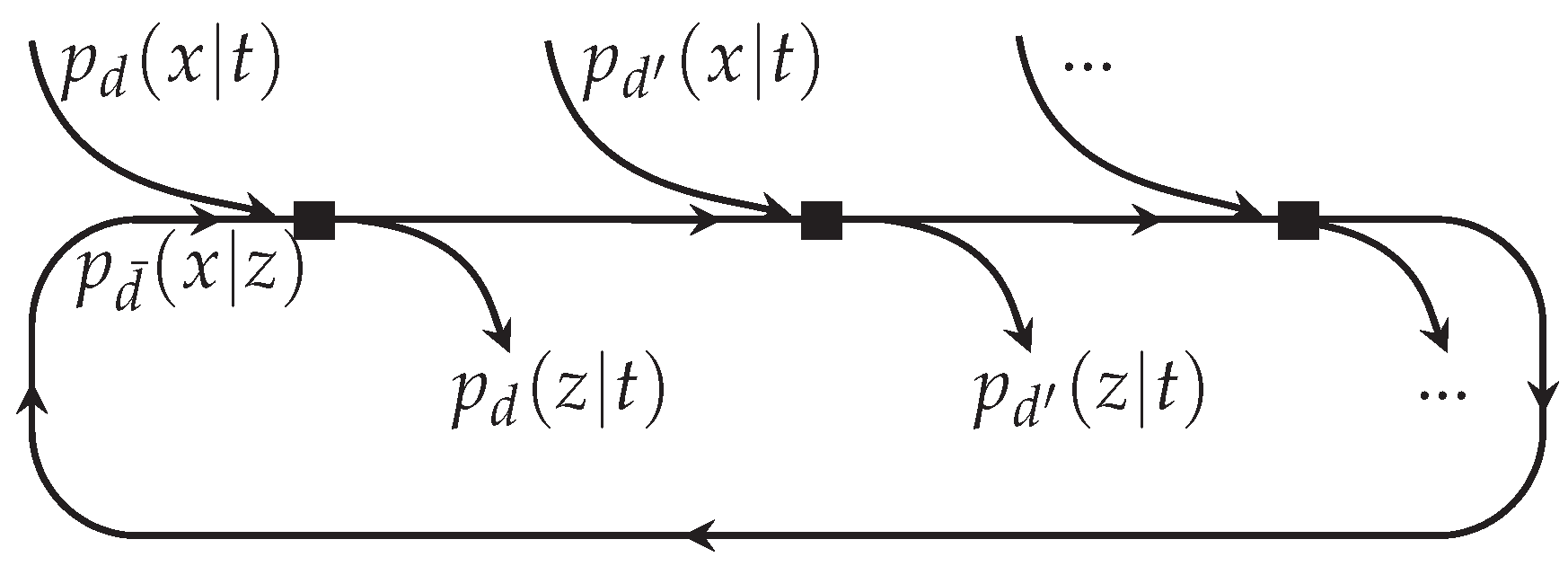
3.4. Message Alignment—A Graphical Perspective

In this subsection, some consequences of Definition (4) will be sketched, resulting in what we call the message alignment problem. Please recall that LLRs are not needed in the entire information bottleneck decoder during decoding, because only cluster indices t are exchanged. However, analyzing LLRs interpretation of a particular cluster index t in density evolution allows the limiting factor of the considered decoding method to be graphically illustrated for irregular codes. Figure 5a visualizes the meanings of certain cluster indices t with respect to x before and after averaging over the degree distribution according to (4). Here, $L_2\left(x\right|t)=\log \frac{p_2(X=0|t)}{p_2(X=1|t)}$ and $L_4\left(x\right|t)=\log \frac{p_4(X=0|t)}{p_4(X=1|t)}$ denote the conveyed meanings of a certain cluster t with respect to x of variable nodes with degree two and four before, that is, without averaging according to (4).

Both compression variables have the same event space $\mathcal{T}$. However, the meaning conveyed by a certain cluster with respect to X differs. This means that the cross and dot for the same index t in Figure 5a do not superimpose. For instance, if $t=13$ and $d=2$, $L_2\left(x\right|t)\approx 2.88$ and if $d=4$, $L_4\left(x\right|t)\approx 4.02$ (cf. arrows in Figure 5a). After application of (4), the averaged meaning, that is, $L_{\overline{d}}\left(x\right|t)=\log \frac{p_{\overline{d}}(X=0|t)}{p_{\overline{d}}(X=1|t)}$ (cf. black triangles in Figure 5a) lies somewhere in between and neither matches the originally intended belief of the variable node with degree two nor the one with degree four. Nevertheless, a closer look at Figure 5a leads to another interesting observation. Although the meanings corresponding to the same indices can differ significantly (i.e., $L_2\left(x\right|T=t)\ne L_4\left(x\right|T=t)$), quite similar meanings are expressed by different cluster indices. That is, $L_2\left(x\right|T=t_2)\approx L_4\left(x\right|T=t_4)$ for some $t_2\ne t_4$. The explanation of this phenomenon is as follows. The clusterings $p_d\left(t\right|\mathbf{y})$ are determined independently for different d. Although by construction the realizations of the compression variables $t_d\in \mathcal{T}$ coincide, the realizations have no natural or physical interpretation which enable a meaningful order or relation (e.g., between $t_2\in {\mathcal{T}}_2$ and $t_4\in {\mathcal{T}}_4$). In other words, the messages are not aligned with respect to their belief on x. We advocate that this misalignment inhibits a straightforward application of (4). Therefore, knowing the node degrees d is extremely important to recapture $L_d\left(x\right|t)$. However, this node degree is not available at a receiving node in message passing decoding. At this point, we defer further evidence to Section 5, where it is shown that information bottleneck decoders without message alignment exhibit a notable performance degradation.

3.5. Message Alignment—An Information-Theoretic Perspective

In Figure 5a we noted by comparing the cross and dot markers that providing the node degree d together with the respective cluster index t is required to recover the proper belief on the relevant bit X. However, this approach would result in a very impractical decoder that is tailored to the actual connections between variable nodes and check nodes in a particular code. We propose to solve the underlying message alignment problem using information-theoretical concepts. Therefore, in this subsection, we first derive an information-theoretic formulation of the message alignment problem.

From an information theoretic point of view, $I(X;T,D)$ upper-bounds the information on X of a node receiving an incoming discrete message t. Rewriting $I(X;T,D)$ using the chain rule of mutual information yields

$$I(X;T,D)=I(X;D|T)+I(X;T),$$

(5)

where $I(X;T)$ is the information about X obtained by receiving T alone and $I(X;D|T)$ is the additional information gained by also providing the node degree if the cluster index is already known. In turn, if $I(X;D|T)\approx 0$, from an information-theoretic point of view, conveying the delivering node degree d in addition to the cluster index yields no information gain about X. Thus, we propose a message mapping construction which minimizes $I(X;D|T)$ such that exchanging the node degree in addition to the cluster index yields no information gain. Expanding $I(X;T,D)$ for a variable node yields

$$\begin{array}{cc}\hfill I(X;D|T)& =\sum _{t\in \mathcal{T}}\sum _{d=2}^{{\omega }_{\max }}{\omega }_d{p}_d\left(t\right)D_{KL}\{p_d\left(x\right|t)\left|\right|p_{\overline{d}}\left(x\right|t)\}\hfill \end{array}$$

(6)

$$\begin{array}{cc}& ={\mathbb{E}}_{t,d}\left[D_{KL}\{p_d\left(x\right|t)\left|\right|p_{\overline{d}}\left(x\right|t)\}\right],\hfill \end{array}$$

(7)

where $D_{KL}\{.\Vert .\}$ denotes the Kullback–Leibler divergence.

The result from (7) has a direct intuitive link to Figure 5a. If the cross and dot markers would nearly superimpose for a particular cluster, the change in meaning introduced by averaging would be negligible. Similarly, in this case the Kullback–Leibler divergence between $p_d\left(x\right|t)$ and $p_{\overline{d}}\left(x\right|t)$ would also be small. If this holds on average for all clusters and node degrees, $I(X;D|T)\approx 0$. Motivated by the observation that similar meanings are expressed by different cluster indices paired with (7), our general idea is to map the different $t_d$ onto a variable $z_d$ such that the meanings $p_d\left(x\right|z)$ are aligned. Consequently, we define message alignment as a reordering strategy described by a deterministic mapping $p_d\left(z\right|t)$ to obtain

$$\underset{p_d\left(z\right|t)}{\min }{\mathbb{E}}_{z,d}\left[D_{KL}\{p_d\left(x\right|z)\left|\right|p_{\overline{d}}\left(x\right|z)\}\right],\forall d.$$

(8)

That is, message alignment assigns those indices $t_d$ with meanings $p_d\left(x\right|t)$ to a new cluster index $z_d$ which represents approximately the same meaning with respect to X. Figure 5b depicts the aligned meanings after application of the message alignment algorithm presented in the next subsection. As a consequence, $I(X;D|Z)\approx 0$ and now z instead of t is exchanged over the edges of the Tanner graph.

3.6. Message Alignment Algorithm

To the best of our knowledge, due to the structure of (8) and the restriction to deterministic mappings $p_d\left(z\right|t)$, deriving an optimal implicit solution for (8) is not possible. In the literature, iterative algorithms have been proposed to minimize problems involving the Kullback–Leibler divergence [29]. Thus, we propose an iterative algorithm as depicted in Figure 6.

First, only the independently generated mappings for each node degree and the corresponding degree-specific cluster meanings $p_d\left(x\right|t)$ exist. The black squares in Figure 6 depict the actual message alignment steps. According to (8), in each step, a particular $p_d\left(x\right|t)$ is aligned with respect to the beliefs of the average distribution $p_{\overline{d}}\left(x\right|z)$ (cf. Figure 6). To start the algorithm, $p_{\overline{d}}\left(x\right|z)$ is initialized with an arbitrary mapping. To find a reordering $p_d\left(z\right|t)$ minimizing (8), a search over all candidates t for the best new cluster index z is performed. That is,

$$z=\arg \underset{z^{\ast }}{\min }{D}_{\mathrm{KL}}\left\{p_d\left(x\right|T=t)\left|\right|p_{\overline{d}}\left(x\right|Z=z^{\ast })\right\},\forall t,$$

(9)

which yields $p_d\left(z\right|t)$. Afterwards, $p_d\left(x\right|z)$ is computed using the determined $p_d\left(z\right|t)$. Then, $p_{\overline{d}}(x,z)$ is updated similar to (4), but considering only the weights ${\omega }_d$ of the already-aligned nodes. As visualized in Figure 6, this averaged distribution $p_{\overline{d}}\left(x\right|z)$ is forwarded and serves as new input in the next alignment step, together with $p_{d^{\prime }}\left(x\right|t)$—that is, the not-aligned cluster meanings of a different node with degree $d^{\prime }$. Again, the search according to (9) is performed. Once $p_{d^{\prime }}\left(z\right|t)$ is found, the averaged meaning is updated and forwarded. This processes, as shown in Figure 6, is performed for all node degrees and is repeated iteratively.

Once stable solutions for all message alignment mappings $p_d\left(z\right|t)$ are determined, the final average joint distribution $p_{\overline{d}}(x,z)$ is computed:

$$p_{\overline{d}}(x,z)=\sum _{d=2}^{{\omega }_{\max }}{\omega }_d\sum _{t\in \mathcal{T}}\sum _{\mathbf{y}\in {\mathcal{Y}}_d^{\mathrm{vec}}}{p}_d\left(z\right|t)p_d\left(t\right|\mathbf{y})p_d(x,\mathbf{y}).$$

(10)

This distribution is passed in discrete density evolution and leveraged to design the relevant-information-preserving mappings.

Figure 5b visualizes the LLRs $L_2\left(x\right|z)$ and $L_4\left(x\right|z)$, that is, $L_2\left(x\right|t)$ and $L_4\left(x\right|t)$ after applying the deterministic mapping $p_2\left(z\right|t)$ and $p_4\left(z\right|t)$ which where found using the algorithm described above. The LLRs are now aligned (i.e., $L_2\left(x\right|z)\approx L_4\left(x\right|z)$). Consequently, the average LLR $L_{\overline{d}}\left(x\right|z)$ is quite similar to $L_2\left(x\right|z)$ and $L_4\left(x\right|z)$ (i.e., the original beliefs can propagate through the Tanner graph without significant distortion). The next section investigates how this reduced distortion improves the decoding performance compared to information bottleneck decoders designed without message alignment. The look-up tables used while decoding are $p_d\left(z\right|\mathbf{y})={\sum }_{t\in \mathcal{T}}{p}_d\left(z\right|t)p_d\left(t\right|\mathbf{y})$.

We advocate that message alignment does not affect the implementation complexity of an information bottleneck decoder. The look-up tables $p_d\left(z\right|\mathbf{y})$ have the same size as $p_d\left(t\right|\mathbf{y})$, and z instead of t is exchanged over the edges of the Tanner graph. Thus, introducing message alignment neither increases the number of needed lookup operations, nor does it increase the number of required lookup tables. However, when constructing the lookup tables offline, the message alignment algorithm has to be incorporated in the construction step. This results in slightly increased computational complexity of the construction process compared to the construction of information-bottleneck decoders without message alignment.

4. Optimizing the Node Structure

In this section we devise an optimized structure of the information-bottleneck nodes. First, the general internal processing of the variable nodes and check nodes described in [10] is reviewed. We show that with this design approach the number of required look-up tables and look-up operations depends linearly on the node degree. Especially for LDPC codes with a high code rate, where check nodes with very high degree exist, this linear relation affects the latency tremendously. Our proposed novel tree-like look-up strategy enables a more efficient decoding in terms of space complexity and latency.

Figure 1 depicts message passing decoding in a Tanner graph. Depending on the node type, the M incoming discrete messages $\mathbf{y}={[y_1,\cdots ,y_M]}^{\mathrm{T}}$ are processed in different ways to generate an outgoing message t. In general, it is possible to plug the joint distribution $p(x,\mathbf{y})$ as input distribution in the information bottleneck algorithm. However, the vector $\mathbf{y}$ with M entries, all taken from the discrete alphabet $\mathcal{Y}$, can take up to ${\left|\mathcal{Y}\right|}^M$ distinct combinations. In turn, a huge look-up table $p\left(t\right|\mathbf{y})$ with ${\left|\mathcal{Y}\right|}^M$ entries needs to stored. Even for small node degrees, this exponential growth of entries prohibits a direct practical implementation. This problem is tackled by partitioning the equality constraint at the variable nodes and the (mod 2)-sum at the check nodes into a serial concatenation of simple partial operations with only two inputs. Such a so-called opened node is illustrated in Figure 7a.

Due to the sequential concatenation of look-up tables, $M-1$ different tables are required in each iteration and for each node degree. Since only two incoming discrete messages are used at a time, the size of the look-up table is ${\left|\mathcal{Y}\right|}^2$. Thus, instead of one large table with ${\left|\mathcal{Y}\right|}^M$ entries, in total $(M-1)·{\left|\mathcal{Y}\right|}^2$ entries need to be stored for a decoder designed as in [10]. While decoding using the sequential design, $M-1$ look-up operations have to be performed.

The code rate of regular LDPC codes is $R=1-\frac{d_v}{d_c}$, where $d_v$ is the variable node degree and $d_c$ denotes the check node degree. Consequently, to achieve a high code rate, very large check node degrees are required. In optical communications, often $d_c>20$. Hence, the sequential design is very inefficient in terms of memory demand and latency due to the large number of required look-up tables. Instead, we propose a more efficient look-up strategy that requires fewer tables. The proposed design is sketched in Figure 7b. We denote the stage of the look-up tree with s. We note that when using a tree-like pattern, the depth of the information bottleneck graph is reduced from $\mathcal{O}(M-1)$ to $\mathcal{O}(2·⎣{\log }_2\left(M\right)⎦)$. The proposed tree-like structure makes use of the following observation: Since the look-up table depends only on the joint distribution which is the same if the “type” of incoming message is the same, it can be reused for the entire stage. That is, in the first stage (i.e., $s=1$), always to incoming messages $y_{2i},y_{2i+1}$ are combined which have the same probability distribution and thus yield the same joint distribution no matter which particular incoming messages $y_i$ are considered. In the next stage (i.e., $s=2$), the inputs to the look-up table are the result of the compression and respectively the look-up from the previous stage (i.e., $t_{1,i}$). Thus, these messages again have the same distribution and thus have the same joint distribution. This procedure continues until the final stage $s={\log }_2\left(M\right)$ is reached. In case M is not a power of two, at most $2·⎣{\log }_2\left(M\right)⎦$ look-up stages are needed. See Appendix A for a detailed derivation. The algorithm to determine the actual number of needed stages if M is not a power of two is also given in Appendix A.

Table 1. Overview of maximum required look-up tables and their sizes depending on the node structure.

Node Structure	Entries per Table	Look-Up Tables	Total Memory Demand
direct	${\left|\mathcal{Y}\right|}^M$	1	${\left|\mathcal{Y}\right|}^M$
sequential propagation	${\left|\mathcal{Y}\right|}^2$	$M-1$	$(M-1)·{\left|\mathcal{Y}\right|}^2$
proposed (tree-like)	${\left|\mathcal{Y}\right|}^2$	$2·⎣{\log }_2\left(M\right)⎦$	$2·⎣{\log }_2\left(M\right)⎦·{\left|\mathcal{Y}\right|}^2$

contains an overview of the required memory depending on the chosen node structure.

Reusing Intermediate Results

In information-bottleneck decoders, the actual decoding simplifies to look-up operations in the offline-generated tables. To compute an outgoing message, all incoming messages, except for the one received over the edge connected to the node we generate the outgoing message for, are considered. Hence, all outgoing messages are computed using a slightly different input vector $\mathbf{y}$. However, parts of the input vector do not change for several outgoing messages. Thus, the total number of look-up operations per node can be reduced by the reuse of intermediate results.

Assuming a sequential node structure, we note that for example if only $y_M$ is changed, all $t_i$ for $i=0,\cdots ,M-2$ previous results could be reused. Thus, the number of total operations for all outgoing edges for a node with M incoming messages can be found as

$$(M+1)·(M-1)-\sum _{i=1}^{M-2}i=\frac{(M-1)(M+4)}{2}.$$

By exploiting the proposed tree structure, the number of look-up operations per node can be reduced even further compared to the sequential approach. The actual reuse potential depends largely on the internal structure of the tree. However, in the worst case, $\mathcal{O}(M⎣{\log }_{2}M⎦)$ operations per node are required. In the next section, the achievable gains in terms of latency and memory efficiency are investigated.

5. Investigation and Results

In this section, we apply message alignment and the proposed tree-like node structure during the construction of information-bottleneck decoders for irregular LDPC codes. The investigated irregular code is taken from [3], where several irregular LDPCs relevant for optical communications were proposed and compared. We provide numerical simulations for our proposed information bottleneck decoder and several reference systems assuming transmission over an additive white Gaussian noise (AWGN) channel with BPSK modulation. We compare the decoder in terms of decoding performance, computational complexity, and memory demand.

5.1. Code Properties

The considered code had a length of $N=8000$ bits, code rate $R=0.8$, and the degree distribution [3]:

$$\begin{array}{cc}\hfill \rho \left(z\right)& =0.7z^{22}+0.3z^{23},\hfill \end{array}$$

(11)

$$\begin{array}{cc}\hfill \lambda \left(z\right)& =0.150z^2+0.314z^3+0.536z^{12}.\hfill \end{array}$$

(12)

5.2. Memory Demand

Given the degree distribution from [3], an information bottleneck decoder can be constructed as proposed in Section 3. We designed the decoder to perform at most $i=50$ iterations. That is, $i=50$ different tables for each node degree and node type have to be generated. For the considered code,

Table 2. Overview of the number of look-up table entries and the total memory demand depending on the node structure.

Node Degree	Direct		Sequential		Proposed (Tree-Like)
	Entries	Look-Ups	Entries	Look-Ups	Entries	Look-Ups
$d_v=2$	4096	2	512	3	512	3
$d_v=3$	$65,536$	3	768	7	512	6
$d_v=12$	$450.35·{10}^{11}$	12	3072	88	1280	33
$d_c=22$	$309.48·{10}^{22}$	22	5376	250	1536	70
$d_c=23$	$495.48·{10}^{23}$	23	5632	273	1536	92
Total per Iteration	$525.931·{10}^{23}$	62	$15,360$	621	5376	204
Total for $i=50$	$209.2·{10}^{27}$	3100	$768,000$	31,050	$268,800$	10,200
Memory for $i=50$ in kByte	$104.6·{10}^{24}$	-	384	-	$134.4$	-

summarizes the memory demand. Clearly, the direct implementation with only one look-up table per iteration and node degree is not implementable due to the huge memory requirement of 104.6 ·${10}^{24}$ kByte. The sequential approach proposed in [10] already yields a manageable complexity and allows the construction of an information bottleneck decoder that only needs 384 kByte of memory in total. Please note that due to very simple look-up operations leveraged for decoding, other than in conventional LDPC decoders, not the computational complexity but the memory demand and the memory access times are the only parameters affecting the space complexity and decoding throughput. Thus, it is crucial that the number of look-ups is reduced and parallelized to simultaneously tackle decoding speed and memory demand. Table 2 shows that the proposed tree-like node structure also achieved notable improvements for practically relevant codes. In total, only $134.4$ kByte memory were required to realize the entire information bottleneck decoder. This is a reduction of $65\%$. Furthermore, the number of distinct look-up tables for the node with highest degree (i.e., the check node with $d_c=23$) could be reduced from 21 to 6, which is a reduction by $71\%$. Table 2 also includes the total number of look-ups needed to compute all outgoing messages per node and iteration. Clearly, the tree-like structure needs significantly less operations compared to the sequential structure, which enhances the decoding speed correspondingly.

5.3. Bit Error Rate (BER) Performance

For performance evaluation, BER curves for three conventional decoders and two information bottleneck decoders are shown in Figure 8. All compared systems performed at most $i=50$ decoding iterations or stopped if the syndrome check was satisfied. The properties of the decoders used are summarized in

Table 3. Properties of the compared decoding algorithms.

Decoder	Node	Messages	Messages	Message
	Operations	(Internal)	(Channel)	Alignment
belief propagation	arithmetic	64 bit	64 bit	-
belief propagation, quantized channel output	arithmetic	64 bit	4 bit	-
min-sum	approx. arithmetic	64 bit	64 bit	-
information-bottleneck decoder [10]	look-up Table	4 bit	4 bit	no
proposed	look-up table	4 bit	4 bit	yes

.

The first reference decoder (cf. dash-dotted blue curve in Figure 8) was a belief propagation decoder which receives quasi-continuous LLRs from the channel and performs box-plus operations at the check nodes and summations at the variable node. Clearly, the processing of quasi-continues LLRs in a digital implementation also requires very fine quantization. Standard processor architectures approximate the processing of continuous signal using floating-point or double-precision data types.

In a second step, we included a 4-bit channel output quantizer as described in [18] in our simulation. The belief propagation decoder receives only 16 distinct LLRs from the quantizer. However, the internal processing still uses quasi-continuous LLRs. We denote this approach “belief propagation decoding with quantized channel output” (cf. dashed green curve in Figure 8).

The third considered decoding approach was min-sum decoding (cf. dotted red curve in Figure 8). Just like the belief propagation decoder, the min-sum decoder receives channel LLRs which are not quantized and need to be represented precisely. These LLRs were exchanged during message passing decoding. However, the box-plus operation at the check node was approximated in min-sum decoding and thus much simpler compared to box-plus.

The aim of information bottleneck decoders is to combine both domains (i.e., simple node operations and compressed messages) such that only a small number of bits has to be exchanged. We restricted the cardinality of the compression variable T to 4 bits.

The solid magenta curve with “o” markers in Figure 8 corresponds to our proposed information bottleneck decoder, which uses message alignment during the construction. When constructed without message alignment, the information bottleneck decoder (cf. solid light-blue curve with “x”-markers) diverged already at a BER of $5·{10}^{-3}$. In contrast, the results obtained with our proposed information bottleneck decoder were quite remarkable compared to the performance of a belief propagation decoder working with double-precision data types. Although only 16 different integers were processed by the information bottleneck decoder, the performance degradation in terms of bit error rate was only 0.15 dB for a BER of ${10}^{-3}$ down to ${10}^{-5}$. The operations performed during information-bottleneck decoding were only simple look-ups in the offline-generated look-up tables, whereas the belief propagation reference simulation processed double precision channel output values and also performed double precision box-plus operations.

The performance degradation was even smaller if the belief propagation decoder with quantized channel LLRs was considered as reference. It suffered from the same information loss introduced by using the channel quantizer as the information-bottleneck decoder. Finally, although the min-sum decoder exchanges double precision LLRs, the performance was significantly worse compared to our proposed information-bottleneck decoder. As a consequence, the performance gain achieved by applying message alignment allows the construction of information bottleneck decoders for irregular LDPC codes which pair coarse quantization, low complexity, simple node operations, and close-to-optimum performance.

6. Conclusions

In this paper, we generalized the construction of an information bottleneck decoder to be also applicable for arbitrary irregular LDPC codes with arbitrary rates. For this purpose, we first extended discrete density evolution for irregular codes and revealed that due to the discrete and finite alphabets of the compression variables, a straightforward application of existing methods is not possible without an additional processing step. We derived the underlying information-theoretic optimization problem and devised a solution, which we call message alignment. By adding this extra step, we were able to build a 4-bit information bottleneck decoder in which all arithmetic operations were replaced by look-up tables mapping incoming 4-bit messages onto outgoing 4-bit messages. Our presented decoder is characterized by a significantly lower implementation complexity than conventional decoders. However, at the same time, the information-bottleneck decoder achieved a comparable performance (0.15 dB gap) to double-precision belief propagation and significantly better performance than min-sum decoders. To achieve a design with low latency and less memory demand, a tree-like node structure was superior. With this structure, the memory to store the look-up tables depends only logarithmically $\left(\mathcal{O}(2·⎣{\log }_2\left(M\right)⎦)\right)$ on the number of processed messages M instead of linearly $\left(\mathcal{O}\right(M-1\left)\right)$. A similar improvement was achieved when considering the number of performed look-up operations. We believe that the demonstrated applicability now also for practically relevant irregular LDPC codes with arbitrarily high rates increases the relevance of information bottleneck decoders as promising candidates for practically important finite-precision LDPC decoding in the context of optical communications.

References

1. Chung, S.Y.; Forney, G.D.; Richardson, T.J.; Urbanke, R. On the design of low-density parity-check codes within 0.0045 dB of the Shannon limit. IEEE Commun. Lett. 2001, 5, 58–60. [Google Scholar] [CrossRef] [Green Version]
2. Chang, D.; Yu, F.; Xiao, Z.; Li, Y.; Stojanovic, N.; Xie, C.; Shi, X.; Xu, X.; Xiong, Q. FPGA Verification of a Single QC-LDPC Code for 100 Gb/s Optical Systems without Error Floor down to BER of 10−15. In Proceedings of the 2011 Optical Fiber Communication Conference/National Fiber Optic Engineers Conference, Los Angeles, CA, USA, 6–10 March 2011; OSA: Washington, DC, USA, 2011; p. OTuN2. [Google Scholar] [CrossRef]
3. Koike-Akino, T.; Millar, D.S.; Kojima, K.; Parsons, K.; Miyata, Y.; Sugihara, K.; Matsumoto, W. Iteration-Aware LDPC Code Design for Low-Power Optical Communications. J. Lightw. Technol. 2016, 34, 573–581. [Google Scholar] [CrossRef]
4. Schmalen, L.; Suikat, D.; Rosener, D.; Aref, V.; Leven, A.; ten Brink, S. Spatially coupled codes and optical fiber communications: An ideal match? In Proceedings of the 2015 IEEE 16th International Workshop on Signal Processing Advances in Wireless Communications (SPAWC), Stockholm, Sweden, 28 June–1 July 2015; IEEE: Piscataway, NJ, USA, 2015; pp. 460–464. [Google Scholar] [CrossRef] [Green Version]
5. Sugihara, K.; Miyata, Y.; Sugihara, T.; Kubo, K.; Yoshida, H.; Matsumoto, W.; Mizuochi, T. A Spatially-coupled Type LDPC Code with an NCG of 12 dB for Optical Transmission beyond 100 Gb/s. In Proceedings of the 2013 Optical Fiber Communication Conference/National Fiber Optic Engineers Conference, Anaheim, CA, USA, 17–21 March 2013; OSA: Washington, DC, USA, 2013; p. OM2B.4. [Google Scholar] [CrossRef]
6. Yang, M.; Ryan, W.E.; Li, Y. Design of Efficiently Encodable Moderate-Length High-Rate Irregular LDPC Codes. IEEE Trans. Commun. 2004, 52, 564–571. [Google Scholar] [CrossRef]
7. Zhou, X.; Xie, C. Enabling Technologies for High Spectral-Efficiency Coherent Optical Communication Networks; John Wiley & Sons, Inc.: Hoboken, NJ, USA, 2016. [Google Scholar]
8. Leven, A.; Schmalen, L. Status and Recent Advances on Forward Error Correction Technologies for Lightwave Systems. J. Lightw. Technol. 2014, 32, 2735–2750. [Google Scholar] [CrossRef]
9. Meidlinger, M.; Matz, G. On irregular LDPC codes with quantized message passing decoding. In Proceedings of the 2017 IEEE 18th International Workshop on Signal Processing Advances in Wireless Communications (SPAWC’17), Sapporo, Japan, 3–6 July 2017; IEEE: Piscataway, NJ, USA, 2017; pp. 1–5. [Google Scholar]
10. Lewandowsky, J.; Bauch, G. Information-Optimum LDPC Decoders Based on the Information Bottleneck Method. IEEE Access 2018, 6, 4054–4071. [Google Scholar] [CrossRef]
11. Lewandowsky, J.; Stark, M.; Bauch, G. Optimum message mapping LDPC decoders derived from the sum-product algorithm. In Proceedings of the 2016 IEEE International Conference on Communications (ICC’16), Kuala Lumpur, Malaysia, 22–27 May 2016; IEEE: Piscataway, NJ, USA, 2016; pp. 1–6. [Google Scholar]
12. Romero, F.J.C.; Kurkoski, B.M. LDPC decoding mappings that maximize mutual information. IEEE J. Sel. Areas Commun. 2016, 34, 2391–2401. [Google Scholar] [CrossRef]
13. Kurkoski, B.M.; Yamaguchi, K.; Kobayashi, K. Noise thresholds for discrete LDPC decoding mappings. In Proceedings of the 2008 IEEE Global Communications Conference, New Orleans, LO, USA, 30 November–4 December 2008; IEEE: Piscataway, NJ, USA, 2008; pp. 1–5. [Google Scholar]
14. Meidlinger, M.; Balatsoukas-Stimming, A.; Burg, A.; Matz, G. Quantized message passing for LDPC codes. In Proceedings of the 2015 49th Asilomar Conference on Signals, Systems and Computers, Pacific Grove, CA, USA, 8–11 November 2015; pp. 1606–1610. [Google Scholar] [CrossRef]
15. Bauch, G.; Lewandowsky, J.; Stark, M.; Oppermann, P. Information-Optimum Discrete Signal Processing for Detection and Decoding. In Proceedings of the IEEE 87th Vehicular Technology Conference (VTC-Spring’18), Porto, Portugal, 3–6 June 2018; IEEE: Piscataway, NJ, USA, 2018. [Google Scholar]
16. Ghanaatian, R.; Balatsoukas-Stimming, A.; Muller, T.C.; Meidlinger, M.; Matz, G.; Teman, A.; Burg, A. A 588-Gb/s LDPC Decoder Based on Finite-Alphabet Message Passing. IEEE Trans. Very Large Scale Integr. (VLSI) Syst. 2018, 26, 329–340. [Google Scholar] [CrossRef] [Green Version]
17. Stark, M.; Lewandowsky, J.; Bauch, G. Information-Optimum LDPC Decoders with Message Alignment for Irregular Codes. In Proceedings of the 2018 IEEE Global Communications Conference: Signal Processing for Communications (Globecom2018 SPC), Abu Dhabi, UAE, 9–13 December 2018; IEEE: Piscataway, NJ, USA, 2018. [Google Scholar]
18. Lewandowsky, J.; Stark, M.; Bauch, G. Message Alignment for Discrete LDPC Decoders with Quadrature Amplitude Modulation. In Proceedings of the 2017 IEEE International Symposium on Information Theory, Aachen, Germany, 25–30 June 2017; IEEE: Piscataway, NJ, USA, 2017; pp. 2925–2929. [Google Scholar]
19. Stark, M.; Lewandowsky, J.; Bauch, G. Iterative Message Alignment for Quantized Message Passing between Distributed Sensor Nodes. In Proceedings of the IEEE 87th Vehicular Technology Conference (VTC-Spring’18), Porto, Portugal, 3–6 June 2018; IEEE: Piscataway, NJ, USA, 2018. [Google Scholar]
20. Ryan, W.; Lin, S. Channel Codes: Classical and Modern; Cambridge University Press: Cambridge, UK, 2009. [Google Scholar]
21. Tishby, N.; Pereira, F.C.; Bialek, W. The information bottleneck method. In Proceedings of the 37th Allerton Conference on Communication and Computation, Monticello, IL, USA, 22–24 September 1999. [Google Scholar]
22. Slonim, N. The Information Bottleneck: Theory and Applications. Ph.D. Thesis, Hebrew University of Jerusalem, Jerusalem, Israel, 2002. [Google Scholar]
23. Hassanpour, S.; Wuebben, D.; Dekorsy, A. Overview and Investigation of Algorithms for the Information Bottleneck Method. In Proceedings of the 11th International ITG Conference on Systems, Communications and Coding, Hamburg, Germany, 6–9 February 2017; VDE: Frankfurt am Main, Germany, 2017; Volume 268. [Google Scholar]
24. Stark, M.; Shah, S.A.A.; Bauch, G. Polar Code Construction using the Information Bottleneck Method. In Proceedings of the 2018 IEEE Wireless Communications and Networking Conference Workshops (WCNCW): Polar Coding for Future Networks: Theory and Practice (IEEE WCNCW PCFN 2018), Barcelona, Spain, 15–18 April 2018; IEEE: Piscataway, NJ, USA, 2018. [Google Scholar]
25. Kern, D.; Kuehn, V. On Compress and Forward with Multiple Carriers in the 3-Node Relay Channel Exploiting Information Bottleneck Graphs. In Proceedings of the 11th International ITG Conference on Systems, Communications and Coding, Hamburg, Germany, 6–9 February 2017; VDE: Frankfurt am Main, Germany, 2017; pp. 1–6. [Google Scholar]
26. Chen, D.; Kuehn, V. Alternating information bottleneck optimization for the compression in the uplink of C-RAN. In Proceedings of the 2016 IEEE International Conference on Communications (ICC), Kuala Lumpur, Malaysia, 23–27 May 2016; IEEE: Piscataway, NJ, USA, 2016; pp. 1–7. [Google Scholar] [CrossRef]
27. Lewandowsky, J.; Stark, M.; Bauch, G. Information Bottleneck Graphs for receiver design. In Proceedings of the 2016 IEEE International Symposium on Information Theory, Barcelona, Spain, 10–15 July 2016; IEEE: Piscataway, NJ, USA, 2016; pp. 2888–2892. [Google Scholar]
28. Kschischang, F.R.; Frey, B.J.; Loeliger, H.A. Factor graphs and the sum-product algorithm. IEEE Trans. Inf. Theory 2001, 47, 498–519. [Google Scholar] [CrossRef]
29. Minka, T. Divergence Measures and Message Passing; Technical Report; Microsoft Research: Cambridge, UK, 2005. [Google Scholar]
Figure 1. Illustration of a Tanner graph and message passing between variable nodes (circles) and check nodes (squares).
Applsci 08 01884 g001
Figure 2. Information bottleneck setup, where I ( X ; T ) is the relevant information, I ( X ; Y ) is the original mutual information, and I ( Y ; T ) is the compression information.
Applsci 08 01884 g002
Figure 3. Example for a factor graph (left) and an information bottleneck Graph (right) of p ( t | y ) , where y = [ y 1 , , y M ] T . The information bottleneck graph compactly describes that t shall keep relevant information on x while compressing all variables in vector y .
Applsci 08 01884 g003
Figure 4. (a) Discrete memoryless channel (DMC) with subsequent quantizer; (b) Information bottleneck graph of the respective information optimum quantizer.
Applsci 08 01884 g004
Figure 5. Averaged and original cluster meaning of variable nodes with degree two and four (a) without and (b) with message alignment.
Applsci 08 01884 g005
Figure 6. Flow graph of iterative message alignment.
Applsci 08 01884 g006
Figure 7. Illustration of an opened node, where all M incoming messages y 1 , y M are clustered (a) sequentially or (b) as proposed, in a tree-like manner.
Applsci 08 01884 g007
Figure 8. Bit error rate (BER) performance of our proposed decoder and reference systems with properties summarized in Table 3. LLR: log-likelihood ratio.
Applsci 08 01884 g008