Dark Solitons in Acoustic Transmission Line Metamaterials

Abstract

We study dark solitons, namely density dips with a phase jump across the density minimum, in a one-dimensional, weakly lossy nonlinear acoustic metamaterial, composed of a waveguide featuring a periodic array of side holes. Relying on the electroacoustic analogy and the transmission line approach, we derive a lattice model which, in the continuum approximation, leads to a nonlinear, dispersive and dissipative wave equation. The latter, using the method of multiple scales, is reduced to a defocusing nonlinear Schrödinger equation, which leads to dark soliton solutions. The dissipative dynamics of these structures is studied via soliton perturbation theory. We investigate the role—and interplay between—nonlinearity, dispersion and dissipation on the soliton formation and dynamics. Our analytical predictions are corroborated by direct numerical simulations.

1. Introduction

A dark soliton is an envelope soliton that has the form of a density dip with a phase jump across its density minimum. This localized waveform is supported on the top of a stable continuous wave background. Since dark solitons are fundamental nonlinear excitations of a universal model, the defocusing nonlinear Schrödinger (NLS) equation, they have been studied extensively in diverse branches of physics. These include chiefly nonlinear optics [1] and Bose–Einstein condensates [2], but also discrete mechanical systems [3], thin magnetic films [4], complex plasmas [5], water waves [6], and so on. The interest of dark solitons arises from the fact that—since they are composite objects, consisting of a background wave and a soliton—they have a number of interesting properties that may find important applications. Indeed, as compared to the bright solitons (which are governed by the focusing NLS equation), they can be generated by a thresholdless process, are less affected by loss and background noise, and are more robust against various perturbations [1,2]. In addition, in optics, dark solitons have potential applications, e.g., in inducing steerable waveguides in optical media, or for ultradense wavelength-division-multiplexing [1].

Recently, important nonlinear effects—including higher harmonic generation [7,8,9], self-demodulation [10,11], and soliton formation [12,13,14,15,16], and others—have attracted much attention in acoustics, and especially in the context of acoustic metamaterials; these are periodic structures—thus featuring dispersion—which are characterized by negative effective parameters, i.e., negative mass density [17] and negative bulk modulus [18]. Usually, such metamaterials are acoustic waveguides loaded with resonators, presenting strong dispersion around the resonance frequency and Bragg band [19,20]. Dissipation naturally plays a key role in such structures, especially in super-absorbing sound materials [21,22] (see also work in Refs. [23,24]). The combination of dispersion and dissipation [20,23,25,26,27] has mainly been investigated in the linear regime; nevertheless, the additional effect of nonlinearity, which is naturally introduced at high acoustic levels has not been studied in detail in acoustic metamaterials. This is also the case of studies on acoustic solitons of various types—pulse-like [12,13] and envelope bright ones [12,14]. As far as dark solitons are concerned, they were predicted to occur in acoustic waveguides loaded with an array with Helmholtz resonators [12], while the effect of dissipation was neglected. To the best of our knowledge, the dissipation-induced dynamics of dark solitons in acoustic metamaterials, has not been investigated so far.

In this work, we analytically and numerically study envelope dark solitons in a one-dimensional (1D) acoustic metamaterial composed of a waveguide featuring a periodic array of side holes. Based on the transmission line (TL) approach, which is widely used in acoustics [28,29,30,31,32], we model this system by a nonlinear dynamical lattice with losses. In the continuum approximation, the latter leads to a nonlinear, dispersive and dissipative wave equation. Employing the multiple scales perturbation method, we derive an effective defocusing nonlinear Schrödinger (NLS) equation which supports dark soliton solutions. The effect of dissipation is also taken into regard, and is studied analytically by means of perturbation theory for solitons [33]. Numerical simulations, at the level of the nonlinear lattice model, are also performed showing a very good agreement with the analytical predictions relying on the NLS picture. The methodology of this work paves the way for relevant studies in double-negative acoustic metamaterials.

The paper is structured as follows. In Section 2, we introduce our setup, derive the 1D nonlinear lattice model, and study the linear properties of the system. In Section 3, we employ the multiple scale perturbation method to obtain the NLS equation and its envelope dark soliton solutions; both the lossless and dissipative cases are studied. Finally, in Section 4, we present our conclusions and discuss some future research directions.

2. Electro-Acoustic Analogue Modeling

2.1. Setup and Model

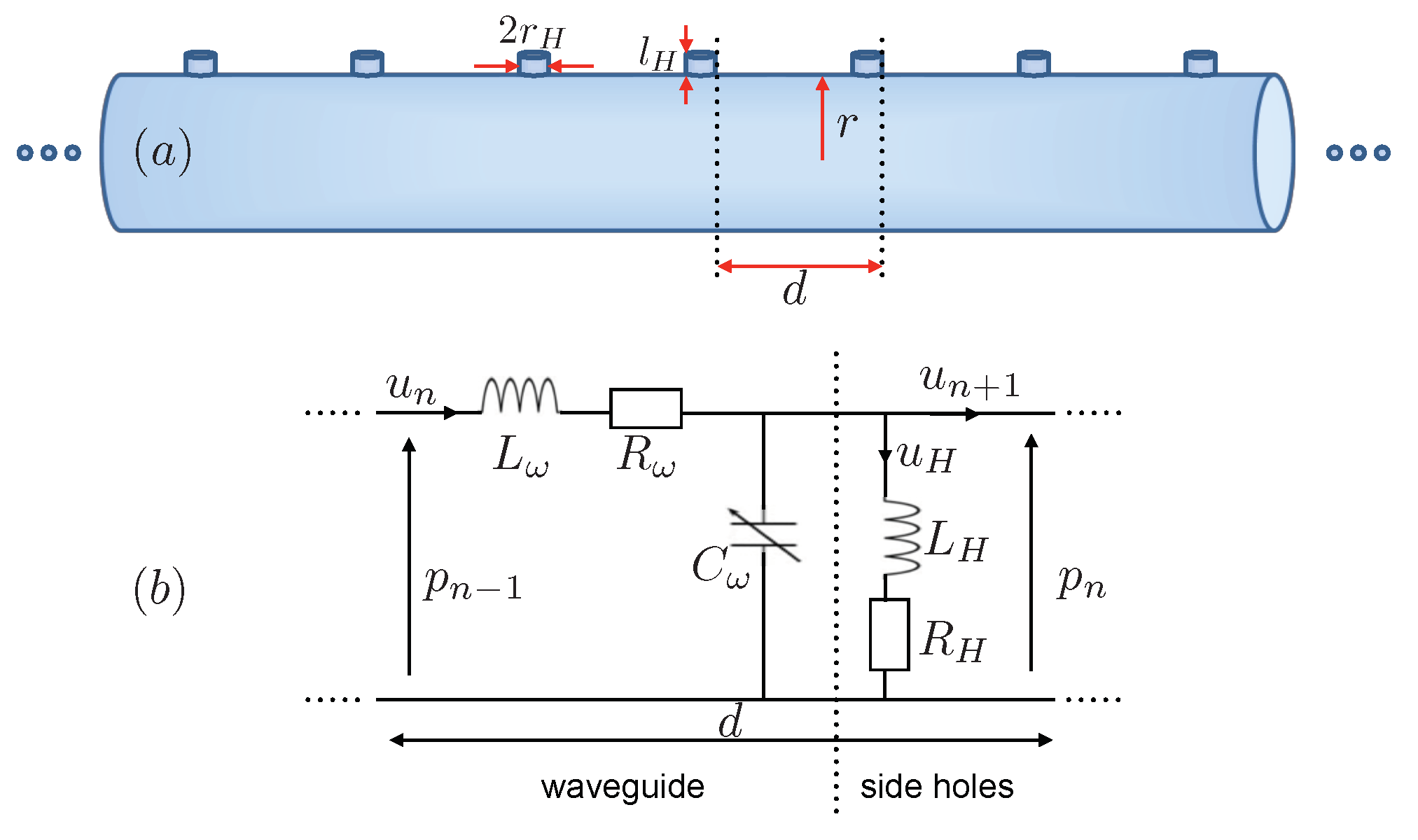
We consider plane wave propagation in a structure composed of a waveguide of radius r periodically loaded with an array of side holes of radius $r_H$ and length $l_H$, and the distance between two consecutive cells is d, as shown in Figure 1a. We choose to work in a frequency range well below the first cut-off frequency of the higher propagating modes in the waveguide, and therefore the problem is considered as 1D.

In order to theoretically analyze the problem, we employ the electro-acoustic analogue modeling based on the transmission line (TL) approach. This allows us to derive a nonlinear, dispersive and dissipative discrete wave equation, which—in the continuum limit—can be treated analytically via the multiple scales perturbation method. The corresponding unit-cell circuit of the TL model is shown in Figure 1b, where the voltage v and the current i correspond to the acoustic pressure p and to the volume velocity u through the waveguide’s cross-sectional area, respectively [12,28].

The first part of the unit-cell circuit, corresponding to the waveguide, is modeled by the inductance $L_{\omega }$, the resistance $R_{\omega }$ and shunt capacitance $C_{\omega }$. The linear part of the inductance and the capacitance are $L_{\omega 0}={\rho }_{0}d/S$ and $C_{\omega 0}=Sd/\left({\rho }_0{c}_0^2\right),$ respectively, where $S=\pi r^2$, ${\rho }_0$ and $c_0$ are the cross section of the waveguide, the density and the sound velocity of the fluid in the system, respectively. We consider weakly nonlinear wave propagation, where the celerity $c_{NL}\approx c_0\left(1+{\beta }_{0}p/{\rho }_0{c}_0^2\right)$, with ${\beta }_0$ being the nonlinear parameter, depends on the amplitude. Thus, we consider the capacitance $C_{\omega }$ to be nonlinear, depending on the pressure p, while the inductance $L_{\omega }$ linear [12]. The pressure-dependent capacitance [14] can be expressed as $C_{\omega }=C_{\omega 0}-C_{\omega }^{{}^{\prime }}{p}_n$, where $C_{\omega }^{{}^{\prime }}=2{\beta }_0{C}_{\omega 0}/\left({\rho }_0{c}_0^2\right)$. The resistance $R_{\omega }=\mathrm{Im}\left(k{Z}_c\right)d$, corresponds to the viscothermal losses at the boundaries of the waveguide wall:

$$k=\frac{\omega }{c_0}\left(1+\frac{1-j}{s}(1+(\gamma -1)/\sqrt{Pr})\right)$$

(1)

is the wavenumber and

$$Z_c=\frac{{\rho }_0{c}_0}{S}\left(1+\frac{1-j}{s}(1-(\gamma -1)/\sqrt{Pr})\right)$$

(2)

is the characteristic impedance of the waveguide, with $\gamma$ being specific heat ratio, $Pr$ the Prandtl number, $s=\sqrt{\omega {\rho }_0{r}^2/\eta }$, and $\eta$ the shear viscosity.

The second part of the unit-cell circuit describes the effects of the holes that are considered to be linear (assuming sufficiently smoothed edges of the holes) [34,35]. The side holes could be modeled by a shunt $LR$ circuit composed of the series combination of an inductance $L_H$ and a resistance $R_H$. We study the regime where the wavelength $\lambda$ of the sound wave is much bigger than the geometric characteristic of the side holes, i.e., $k{r}_H\ll 1$. The corresponding inductance could be given by $L_H={\rho }_0(l_H+\Delta l_{Hi}+\Delta l_{Ho})/S_H$, where $\Delta l_{Hi}$ and $\Delta l_{Ho}$ are length corrections due to the radiation inside the waveguide and to the outer environment, respectively [36,37,38] (see more details in Appendix A) and $S_H$ is the area of the side holes. The resistance $R_H={\rho }_0{c}_0{\left(k{r}_H\right)}^2/\left(2S_H\right)={\rho }_0{\omega }^2/\left(2\pi c_0\right)$ corresponds to the radiation losses to the outer environment and the propagation losses due to viscous and thermal effects in the side holes [36].

Here, we should mention that we approximate the frequency-dependent viscothermal losses of the waveguide and the radiation losses due to the side holes by resistance, $R_{\omega }$ and $R_H$, respectively, with the corresponding constant value fixed at the characteristic frequency of the dark solitons (see below).

We now use Kirchhoff’s voltage and current laws to derive the discrete nonlinear dissipative evolution equation for the pressure $p_n$ in the nth cell of the lattice (see details in Appendix B):

$$\begin{array}{c}\left(L_H\frac{d}{dt}+R_H\right)\left(p_{n+1}-2p_n+p_{n-1}-L_{\omega }{C}_{\omega 0}\frac{d^2{p}_n}{d{t}^2}\right.\hfill \\ \left.-R_{\omega }{C}_{\omega 0}\frac{d{p}_n}{dt}+\frac{1}{2}{L}_{\omega }{C}_{\omega }^{{}^{\prime }}\frac{d^2{p}_n^2}{d{t}^2}+\frac{1}{2}{R}_{\omega }{C}_{\omega }^{{}^{\prime }}\frac{d{p}_n^2}{dt}\right)\hfill \\ -\left(L_{\omega }\frac{d}{dt}+R_{\omega }\right)p_n=0.\hfill \end{array}$$

(3)

2.2. Continuum Limit

We now focus on the continuum limit of Equation (3), corresponding to $n\to \infty$ and $d\to 0$ (but with $nd$ being finite); in such a case, the pressure becomes $p_n\left(t\right)\to p(x,t)$, where $x=nd$ is a continuous variable, and

$$p_{n\pm 1}=p\pm d\frac{\partial p}{\partial x}+\frac{d^2}{2}\frac{{\partial }^{2}p}{\partial x^2}\pm \frac{d^3}{3!}\frac{{\partial }^{3}p}{\partial x^3}+\frac{d^4}{4!}\frac{{\partial }^{4}p}{\partial x^4}+O\left(d^5\right),$$

(4)

i.e., $p_{n+1}-2p_n+p_{n-1}\approx d^2{p}_{xx}+d^4{p}_{xxxx}/12$, where subscripts denote partial derivatives. In order to understand more accurately the dynamics of the system, we keep terms up to order $O\left(d^4\right)$ coming from the periodicity of the side holes [14]. This way, we obtain the corresponding partial differential equation (PDE),

$$\begin{array}{c}\left(L_H\frac{\partial }{\partial t}+R_H\right)\left(d^2\frac{{\partial }^{2}p}{\partial x^2}+\frac{d^4}{12}\frac{{\partial }^{4}p}{\partial x^4}-L_{\omega }{C}_{\omega 0}\frac{{\partial }^{2}p}{\partial t^2}\right.\hfill \\ \left.-R_{\omega }{C}_{\omega 0}\frac{\partial p}{\partial t}+\frac{1}{2}{L}_{\omega }{C}_{\omega }^{{}^{\prime }}\frac{{\partial }^2{p}^2}{\partial t^2}+\frac{1}{2}{R}_{\omega }{C}_{\omega }^{{}^{\prime }}\frac{\partial p^2}{\partial t}\right)\hfill \\ -\left(L_{\omega }\frac{\partial }{\partial t}+R_{\omega }\right)p=0.\hfill \end{array}$$

(5)

It is also convenient to express our model in dimensionless form by introducing the normalized variables $\tau$ and $\chi$ and normalized pressure P, which are defined as follows: $\tau$ is time in units of ${\omega }_B^{-1}$, where ${\omega }_B=\pi c_0/d$ is the Bragg frequency; $\chi$ is space in units of $c_0/{\omega }_B$ and $p=ϵP_{0}P$, where $P_0={\rho }_0{c}_0^2$ and $0<ϵ\ll 1$ is a formal dimensionless small parameter. Then, Equation (5) is reduced to the following dimensionless form:

$$\begin{array}{c}\left({\partial }_{\tau }+{\gamma }_H\right)\left[P_{\tau \tau }-P_{\chi \chi }-\zeta P_{\chi \chi \chi \chi }+{\gamma }_{\omega }{P}_{\tau }-ϵ{\beta }_0{\left(P^2\right)}_{\tau \tau }\right.\hfill \\ \left.-ϵ{\beta }_0{\gamma }_{\omega }{\left(P^2\right)}_{\tau }\right]+m^2{P}_{\tau }+m^2{\gamma }_{\omega }P=0,\hfill \end{array}$$

(6)

where,

$$\begin{array}{c}{m}^2=\frac{S_{H}d}{{\pi }^2{l}_{H}S},{\gamma }_H=\frac{R_H}{{\omega }_B{L}_H},\hfill \\ {\gamma }_{\omega }=\frac{R_{\omega }S}{\pi {\rho }_0{c}_0},\zeta =\frac{{\pi }^2}{12}.\hfill \end{array}$$

(7)

It is interesting to identify various limiting cases of Equation (6). First, in the linear limit $({\beta }_0=0$, or $p^2\ll 1)$, in the absence of side holes ($m^2\to 0$, ${\gamma }_H\to 0$) and without considering viscothermal losses (${\gamma }_{\omega }\to 0$) and higher order spatial derivatives, Equation (6) is reduced to the linear wave equation, $P_{\tau \tau }-P_{\chi \chi }=0$. In the linear limit, in the presence of side holes, in the long wavelength approximation and without considering viscothermal losses (${\gamma }_{\omega }\to 0$), radiation losses (${\gamma }_H\to 0$), and higher order spatial derivatives ($\zeta \to 0$), Equation (6) takes the form of the linear Klein–Gordon equation [39,40], $P_{\tau \tau }-P_{\chi \chi }+m^{2}P=0$. Finally, in the nonlinear lossless regime, and in the absence of sides holes, without considering higher order spatial derivatives, Equation (6) is reduced to the well-known Westervelt equation, $P_{\tau \tau }-P_{\chi \chi }-ϵ{\beta }_0{\left(P^2\right)}_{\tau \tau }=0$, which is a common nonlinear model describing 1D acoustic wave propagation [10].

2.3. Linear Limit

We now consider the linear limit of Equation (6) in order to obtain the dispersion relation of the system. Assuming plane waves of the form $P\propto exp\left[i\right(k\chi -\omega \tau \left)\right]$, we obtain the following complex dispersion relation connecting the wavenumber k and frequency $\omega$,

$$\begin{array}{c}D(\omega ,k)=-i\omega (-{\omega }^2+k^2-\zeta k^4+m^2)-i\omega {\gamma }_H{\gamma }_{\omega }\hfill \\ +{\gamma }_H(-{\omega }^2+k^2-\zeta k^4)+{\gamma }_{\omega }(-{\omega }^2+m^2)=0,\hfill \end{array}$$

(8)

where ${\gamma }_{\omega }$ and ${\gamma }_H$ account for the viscothermal losses in the waveguide and the losses (radiation losses and viscothermal losses) due to the side holes, respectively. In the absence of losses, Equation (8) is reduced to:

$$D(\omega ,k_r)=-{\omega }^2+k_r^2-\zeta k_r^4+m^2=0,$$

(9)

which is the familiar dispersion relation of the linear Klein–Gordon model [39,40], with a higher-order spatial derivative term $\zeta k^4$ accounting for the influence of the periodicity of the system to the dispersion relation. Although this term appears to lead to instabilities for large values of k, in the long-wavelength limit where k is sufficiently small, such instabilities do not occur. For frequencies between $0\le \omega <m$, there is a band gap, and, for $m<\omega <{\omega }_B$, there is a propagating band, with the dispersion curve $\omega \left(k\right)$ having the form of hyperbola (see Figure 2).

Considering that all quantities in the dispersion relation (Equations (8) and (9)) are dimensionless, it is also relevant to express them in physical units. The frequency ${\omega }_{ph}$ and wavenumber $k_{ph}$ in physical units are connected with their dimensionless counterparts through $\omega ={\omega }_{ph}/{\omega }_B$ and $k=k_{ph}c/{\omega }_B$. Then, we rewrite Equation (8) with physical units as follows:

$$\begin{array}{c}(-i\frac{{\omega }_{ph}}{{\omega }_B}+{\gamma }_H)(-\frac{{\omega }_{ph}^2}{{\omega }_B^2}+\frac{k_{ph}^2{c}_0^2}{{\omega }_B^2}-\zeta \frac{k_{ph}^4{c}_0^4}{{\omega }_B^4}-i\frac{{\omega }_{ph}}{{\omega }_B}{\gamma }_{\omega })\hfill \\ -i\frac{{\omega }_{ph}}{{\omega }_B}{m}^2+m^2{\gamma }_{\omega }=0.\hfill \end{array}$$

(10)

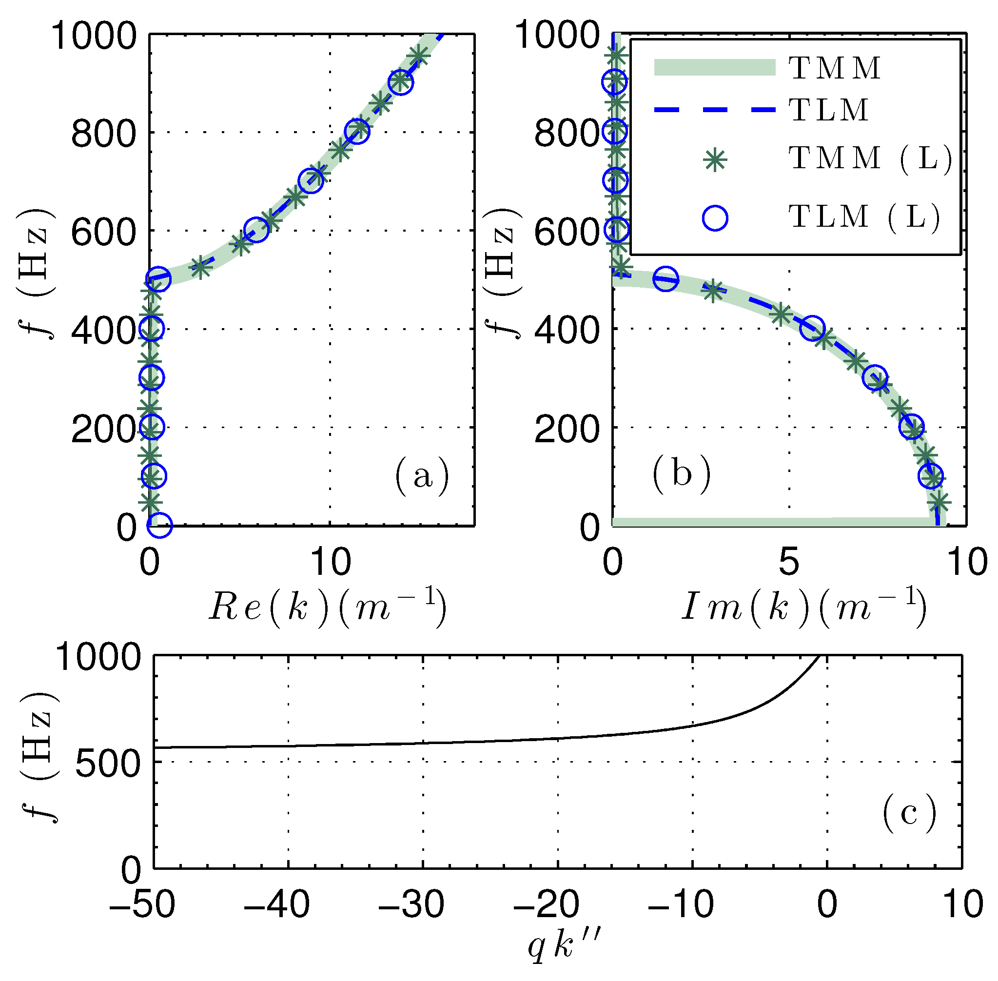
The real and imaginary parts of Equation (10), shown in Figure 2, are found to be almost identical with the lossless case i.e., ${\gamma }_{\omega }=0$ and ${\gamma }_H=0$ (dashed blue lines). Thus, the medium is considered to be weakly lossy. In particular, below we neglect viscothermal losses in the waveguide (${\gamma }_H=0$), which are small compared to radiation losses. Furthermore, we assume that the remaining losses are sufficiently small, such that ${\gamma }_H={ϵ}^2{\gamma }_H^{\prime }$.

On the other hand, the green stars in Figure 2 show the corresponding results for the lossy dispersion relation obtained by using the transfer matrix method (TMM) [20]:

$$cos\left(k_{ph}d\right)=cos\left(kd\right)+i\frac{Z_c}{2Z_H}sin\left(kd\right),$$

(11)

where k and $Z_c$ are given by Equations (1) and (2), respectively, and $Z_H=i{\omega }_{ph}{L}_H+R_H$ is the input impedance of the side holes. For the lossless case, k, $Z_c$ and $Z_H$ are respectively reduced to $k=\omega /c_0$, $Z_c={\rho }_0{c}_0/S$ and $Z_H=i{\omega }_{ph}{L}_H$. The corresponding results are shown as thick green continuous lines in Figure 2. We find that the linear dispersion relation resulting from the TLM is in very good agreement with the one obtained by using the TMM, as shown in Figure 2 in the low frequencies regime.

Here, we mention that results shown in Figure 2 (as well as in Figure 3 and Figure 4 in Section 3 below) are obtained with an air-filled waveguide at 18 °C. We use the following parameter values: $d=0.05$ m, $r=0.025$ m, $r_H=0.005$ m, $l_H=0.002$ m, ${\beta }_0=1.2$, $c_0=343.26$ m/s, ${\rho }_0=1.29$ kg/m${}^3$, $\gamma =C_p/C_v=1.4$, $C_p=1.005$ KJ/kg·K, $C_v=0.718$ KJ/kg·K, $Pr=0.71$ and $\eta =1.84\times {10}^{-5}$ kg/m/s.

3. Dark Solitons

In this section, we use multiple scales perturbation method to describe the evolution of the pressure using an effective lossy NLS equation. From the latter equation, we can obtain the approximate analytical dark soliton solutions of our lattice system and study numerically their dynamics.

We start our analysis by introducing the slow variables,

$${\chi }_n={ϵ}^n\chi ,{\tau }_n={ϵ}^n\tau ,n=0,1,2,\dots ,$$

(12)

and express P as an asymptotic series in $ϵ$,

$$P=p_0+ϵp_1+{ϵ}^2{p}_2+\cdots .$$

(13)

Then, substituting Equations (12) and (13) into Equation (6), we obtain a hierarchy of equations at various orders in $ϵ$ (see more details in Appendix C).

The leading order $O\left({ϵ}^0\right)$, Equation (A8) in Appendix C, possesses a linear plane wave solution of the form

$$p_0=A({\chi }_1,{\chi }_2,\cdots ,{\tau }_1,{\tau }_2,\cdots )exp\left(i\theta \right)+\mathrm{c}.\mathrm{c}.,$$

(14)

where A is an unknown envelop function, $\theta =k_r{\chi }_0-\omega {\tau }_0$ with the wave number $k_r$ and the frequency $\omega$ satisfying the lossless dispersion relation, Equation (9), and c.c. denotes a complex conjugate.

Next, at the order $O\left({ϵ}^1\right)$, the solvable condition is that the secular part (i.e., the term $\propto exp\left(i\theta \right)$) vanishes, which yields,

$$\left(k^{\prime }\frac{\partial }{\partial {\tau }_1}+\frac{\partial }{\partial {\chi }_1}\right)A({\chi }_1,{\chi }_2,\cdots ,{\tau }_1,{\tau }_2,\cdots )=0,$$

(15)

where

$$k^{\prime }=\frac{\partial k}{\partial \omega }=\frac{1}{v_g}=\frac{\omega }{k_r-2\zeta k_r^3},$$

(16)

is the inverse group velocity. Equation (15) is satisfied as long as A depends on the variables ${\chi }_1$ and ${\tau }_1$ through the traveling-wave coordinate ${\tilde{\tau }}_1={\tau }_1-k^{\prime }{\chi }_1$, namely $A({\chi }_1,{\tau }_1,{\chi }_2,{\tau }_2,\cdots )=A({\tilde{\tau }}_1,{\chi }_2,{\tau }_2,\cdots )$. At the same order, we could obtain the form of the field $p_1$,

$$p_1=8{\beta }_0\frac{i{\omega }^3}{D(2\omega ,2k_r)}{A}^2{e}^{2i\theta }+B{e}^{i\theta }+c.c.,$$

(17)

where B is an unknown function that can be found at a higher-order approximation.

Finally, following the same process as above, the nonsecularity condition at $O\left({ϵ}^2\right)$ yields a lossy NLS equation for the envelop function A,

$$i\frac{\partial A}{\partial {\chi }_2}-\frac{1}{2}{k}_r^{″}\frac{{\partial }^{2}A}{\partial {\tilde{\tau }}_1^2}-q{\left|A\right|}^{2}A=-i\mathsf{\Lambda }A,$$

(18)

where the dispersion, nonlinearity and dissipation coefficients are respectively given by,

$$k_r^{″}\equiv \frac{{\partial }^2{k}_r}{\partial {\omega }^2}=\frac{1-k_r^{{}^{\prime }2}+6\zeta k_r^2{k}_r^{{}^{\prime }2}}{k_r-2\zeta k_r^3},$$

(19)

$$q(\omega ,k_r)={\beta }_0^2\frac{4{\omega }^4}{3(m^2+4\zeta k_r^4)(k_r-2\zeta k_r^3)},$$

(20)

$$\mathsf{\Lambda }=\frac{m^2{\gamma }_H^{\prime }}{2\omega (k_r-2\zeta k_r^3)}.$$

(21)

The sign of the product $\sigma \equiv \mathrm{sgn}\left(q{k}^{″}\right)$ determines the nature of the NLS equation [39,40]. A focusing NLS equation with $\sigma =+1$ supports bright solitons, localized waves with vanishing tails towards infinity. A defocusing NLS equation with $\sigma =-1$ supports dark solitons, which are density dips, with a phase jump across the density minimum, on top of a non-vaninishing continuous wave background. Figure 2c shows that the product $q{k}^{″}$ is always negative, i.e., $\sigma =-1$ in our case, which means that our system only supports dark solitons.

In the absence of losses ($\mathsf{\Lambda }=0$), the analytical dark soliton solution for the envelope function A is of the form,

$$\begin{array}{c}A={\eta }_0\left\{b_0\tanh \left[{\eta }_0{b}_0\left(\sqrt{\left|\frac{q}{k_r^{{}^{″}}}\right|}{\tilde{\tau }}_1-a_{0}q{\eta }_0{\chi }_2\right)\right]\right.\hfill \\ \left.+i{a}_0\right\}{e}^{-iq{\eta }_0^2{\chi }_2},\hfill \end{array}$$

(22)

where ${\eta }_0$ is a free parameter setting the amplitude of the dark soliton background, and parameters $a_0=sin\varphi$, $b_0=cos\varphi$ are connected by a relation, $a_0^2+b_0^2=1$, with the effective angle $2\varphi$ corresponding to the phase shift across the dark soliton. The parameter $b_0=cos\varphi$ characterizes the soliton intensity at the center. A black soliton is a special case of a dark soliton, with $\pi$ phase shift and zero intensity at the center. When $\varphi \ne 0$, the minimum intensity of a dark soliton does not equal zero, and we call it a gray soliton.

3.1. Black Solitons

We start with the black soliton, with $\varphi =0$, which at the NLS level is expressed as:

$$A={\eta }_0\tanh \left({\eta }_0\sqrt{\left|\frac{q}{k_r^{{}^{″}}}\right|}{\tilde{\tau }}_1\right)exp\left(-iq{\eta }_0^2{\chi }_2\right).$$

(23)

The corresponding approximate black soliton solution of Equation (6) is as follows:

$$\begin{array}{cc}\hfill P(\chi ,\tau )\approx & 2{\eta }_0\tanh \left[ϵ{\eta }_0\sqrt{\left|\frac{q}{k_r^{{}^{″}}}\right|}\left(\tau -k_r^{\prime }\chi \right)\right]\hfill \\ & \times cos\left(\omega \tau -k_r\chi -{ϵ}^{2}q{\eta }_0^2\chi \right),\hfill \end{array}$$

(24)

which is a function of parameters $\chi$ and $\tau$. In the original coordinates, space x and time t, the approximate black soliton solution for the pressure p reads

$$\begin{array}{cc}\hfill p(x,t)& \approx 2ϵ{\eta }_0{P}_0\tanh \left[ϵ{\eta }_0\sqrt{\left|\frac{q}{k_r^{{}^{″}}}\right|}{\omega }_B\left(t-\frac{k_r^{\prime }}{c_0}x\right)\right]\hfill \\ & \times cos\left(\omega {\omega }_{B}t-\frac{k_r{\omega }_B}{c_0}x-q{ϵ}^2{\eta }_0^2\frac{{\omega }_B}{c_0}x\right),\hfill \end{array}$$

(25)

where $k_r^{\prime }/c_0$ is the inverse group velocity at the carrier frequency that is independent of the amplitude of the background $2ϵ{\eta }_0{P}_0$.

To ensure the balance between nonlinearity and dispersion, we should also pay attention to the dispersion length $L_D$ and the nonlinearity length $L_{NL}$ providing the length scales over which dispersive or nonlinear effects become important for pulse evolution. These lengths are expressed as follows [14]:

$$L_D=\frac{t_0^2{\omega }_B{c}_0}{\left|k_r^{{}^{″}}\right|},$$

(26)

and

$$L_{NL}=\frac{P_0^2{c}_0}{\left|q\right|{\omega }_B{A}_0^2},$$

(27)

where $t_0$ and $A_0$ are the characteristic width and the amplitude of the propagating envelope, respectively. From the black soliton solution, Equation (25), we find $t_0={\left(ϵ{\eta }_0\sqrt{\left|q/k_r^{{}^{″}}\right|}{\omega }_B\right)}^{-1}$ and $A_0=ϵ{\eta }_0{P}_0$. Substituting them in Equations (26) and (27), we obtain $L_{NL}/L_D\sim 1$.

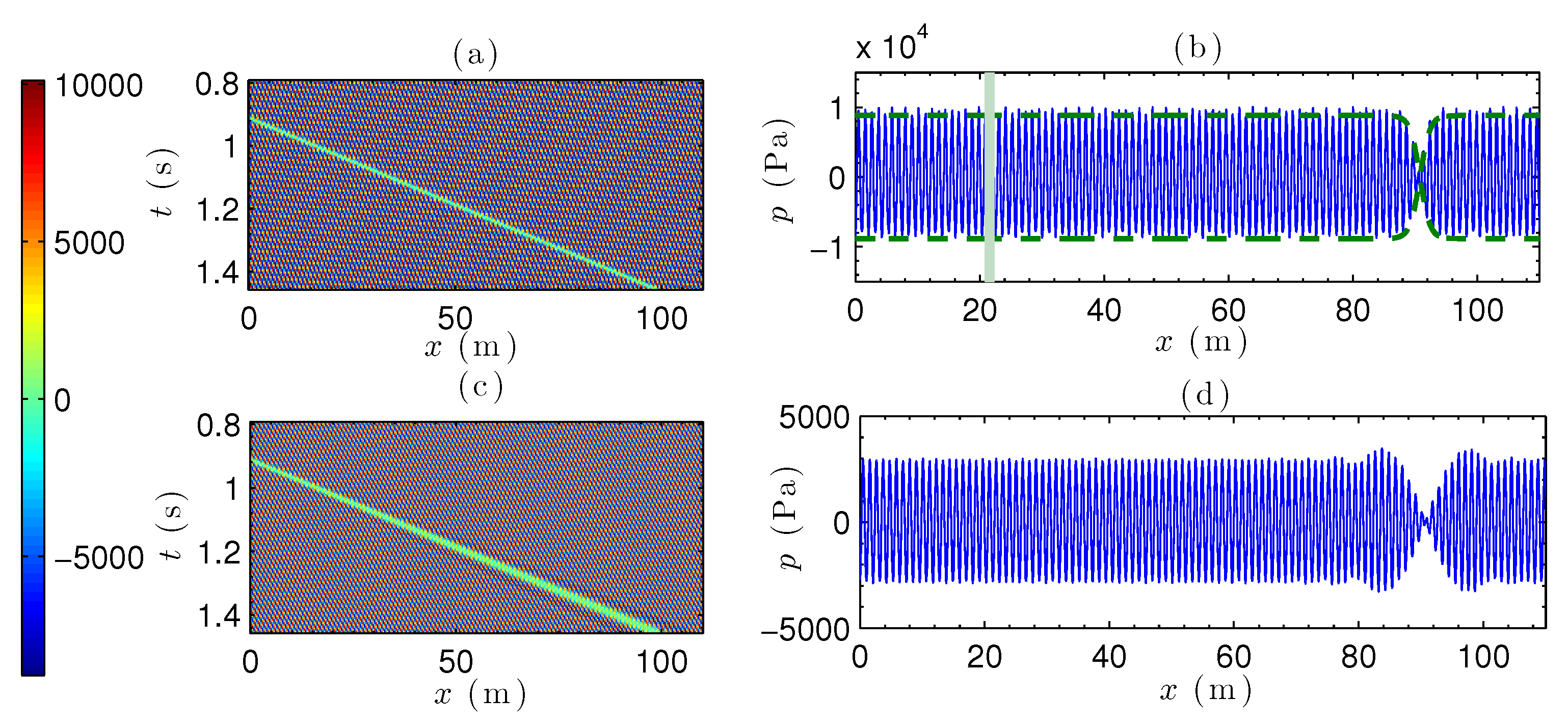
Now, we study numerically the evolution of the approximate black soliton solution of Equation (25) in the lattice. We start by integrating the lossless version of Equation (3) with a driver of the form given by Equation (25) at $x=0$ with $ϵ=0.029$ ($2ϵ\eta P_0=8816$ Pa) (170 dB) and carrier frequency $f=600$ Hz. The numerical results are shown in Figure 3a,b. We observe that the black soliton with zero intensity at the center propagates with a constant velocity, amplitude and width as shown in the contour plot (Figure 3a). Good agreement between the simulations (blue line) calculated at $t=1.41$ s and the corresponding analytical solution of Equation (25) (green dashed line) is shown in Figure 3b. In order to confirm that the black solitons are due to the balance between dispersion and nonlinearity, we also compare Figure 3a,b to the unbalanced case where the boundary condition has the same width but a smaller amplitude, $ϵ=0.0095$ ($2ϵ\eta P_0=2888$ Pa) (160 dB), shown in Figure 3c,d. In Figure 3d, it is observed that the soliton is not formed and the initial wavepacket spreads.

3.2. Black Solitons under Dissipation

We next study the dynamics of the black solitons under the presence of the radiation and viscothermal losses. The effective NLS (18), which includes a linear loss term, can be studied via the direct perturbation theory for dark solitons [33]. The loss term does not vanish for ${\tilde{\tau }}_1\to \infty$ and, thus, in this limit (where ${\partial }^{2}A/\partial {\tilde{\tau }}_1^2\to 0$), the evolution of the black soliton’s background $A\equiv \eta \left({\chi }_2\right)$ is determined by the equation:

$$i\frac{\partial \eta }{\partial {\chi }_2}-q{\left|\eta \right|}^2\eta =-i\mathsf{\Lambda }\eta .$$

(28)

Solutions of Equation (28) can be sought in the form $\eta \left({\chi }_2\right)={\eta }_0\left({\chi }_2\right)exp\left[i\varphi \left({\chi }_2\right)\right]$, where ${\eta }_0\left({\chi }_2\right)$ describes the loss-induced change of the background amplitude, and $\varphi \left({\chi }_2\right)$ is the spatically varying phase of the background. Substituting the above ansatz into Equation (28), and separating real and imaginary parts, we derive the equation for the amplitude of the background as follows:

$$\frac{\partial {\eta }_0}{\partial {\chi }_2}=-\mathsf{\Lambda }{\eta }_0.$$

(29)

Integrating Equation (29), we find that the background amplitude decays according to the following exponential law:

$${\eta }_0\left({\chi }_2\right)={\eta }_0\left(0\right)exp(-\mathsf{\Lambda }{\chi }_2).$$

(30)

In terms of the original space coordinate, the amplitude of the background of the black soliton decreases exponentially as:

$${\eta }_0\left(x\right)={\eta }_0\left(0\right)exp\left(-\frac{x}{L_l}\right),$$

(31)

where

$$L_l=\frac{c_0}{\mathsf{\Lambda }{ϵ}^2{\omega }_B}$$

(32)

is the dissipation length. Thus, the envelope of the approximate black soliton solution reads

$$\begin{array}{c}{p}_e(x,t)\approx 2ϵP_0{\eta }_0\left(0\right)e^{\frac{-\mathsf{\Lambda }{ϵ}^2{\omega }_B}{c_0}x}\hfill \\ \times \tanh \left[ϵ{\eta }_0{e}^{\frac{-\mathsf{\Lambda }{ϵ}^2{\omega }_B}{c_0}x}\sqrt{\left|\frac{q}{k_r^{{}^{″}}}\right|}{\omega }_B\left(t-\frac{k_r^{\prime }}{c_0}x\right)\right].\hfill \end{array}$$

(33)

During propagation, the amplitude of background $\eta$ decreases (due to the presence of loss), while the minimum intensity is always zero. The black soliton does not move against the background, and the velocity of the background only depends on the carrier frequency. Thus, the linear loss only affects the black soliton’s background amplitude and width.

3.2.1. Dissipation Length ≪ Nonlinearity Length and Dispersion Length

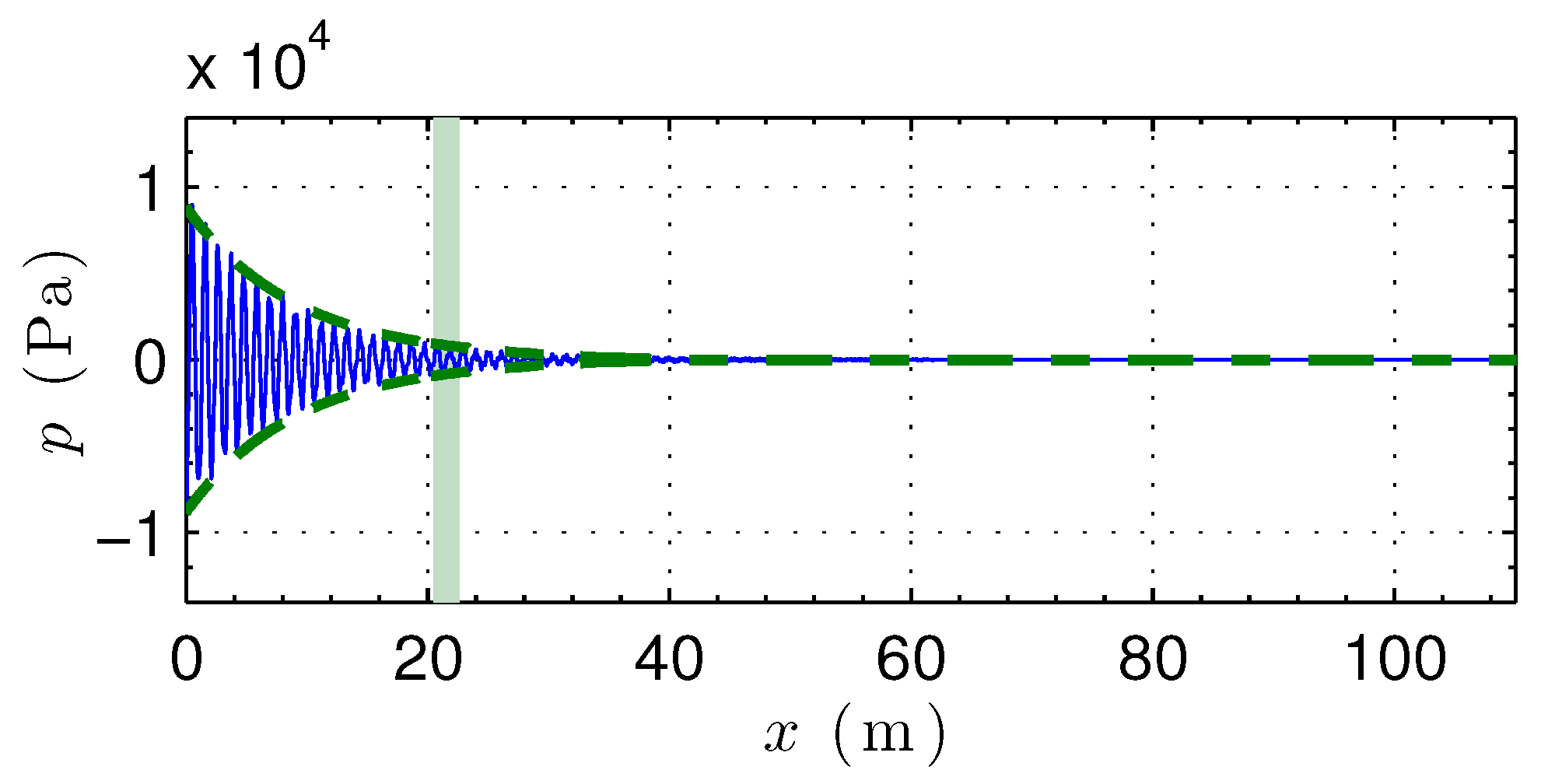
We numerically integrate the lattice model, Equation (3), using a driver corresponding to the black soliton shown in Figure 3 with $ϵ=0.029$ ($2ϵ\eta P_0=8816$ Pa) (170 dB) and $f=600$ Hz. The numerical result (blue line) shown in Figure 4 is in good agreement with the analytical result (green dashed line), Equation (31). The radiation and viscothermal losses strongly attenuate the background amplitude of the black soliton, according to the value of the dissipation length $L_l=9.12$ m, which is much smaller than the nonlinearity and dispersion lengths, given by $L_{NL}=L_D=21.5$ m, illustrated by the light green thick line in Figure 4.

3.2.2. Dissipation Length ≥ Nonlinearity Length and Dispersion Length

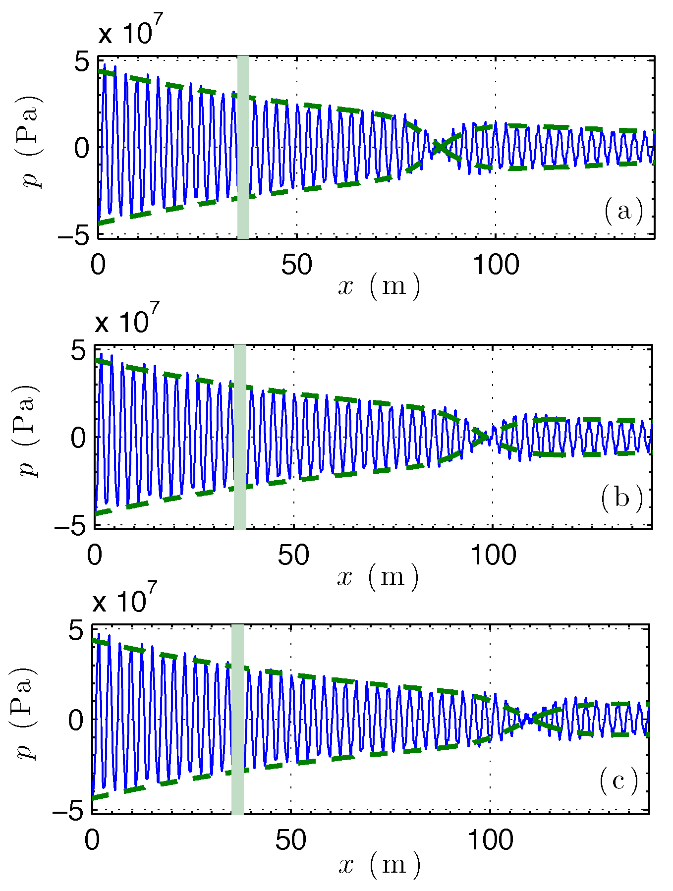
Next, we choose the parameters of our setup so that $L_l\ge L_{NL},L_D$. This is achieved by replacing air to water, and by decreasing the radius of the side holes. We now use the following parameters for the lattice: $d=0.05$ m, $r=0.025$ m, $r_H=0.002$ m, $l_H=0.002$ m, at 25 °C, with nonlinear parameter ${\beta }_0=3.6$, velocity $c_0=1483$ m/s, density ${\rho }_0=998.3$ kg/m${}^3$, specific heat ration $\gamma =C_p/C_v=1.01$, specific heat (constant pressure) $C_p=75.327$ KJ/mol/K, specific heat (constant volume) $C_v=74.53$ KJ/mol/K, Prandtl number $Pr=7.01$ and dynamic viscosity $\eta =1.002{10}^{-3}$ kg/m/s. We use an envelope given by Equation (25) with $ϵ=0.01$ ($2ϵ\eta P_0=4.39\times {10}^7$ Pa) and $f=1300$ Hz. In this case, the background amplitude of the dark soliton is weakly attenuated, and the numerical results (blue lines) are in good agreement with the corresponding analytical ones (green dashed lines) in Figure 5, Equation (31).

Below, we adopt the parameters corresponding to the water-filled acoustic metamaterial.

3.3. Gray Solitons

Apart from the stationary black soliton (characterized by a zero density minimum), there exists the moving gray soliton solution, with $\varphi \ne 0$ (with a nonzero density minimum). The gray soliton solution of Equation (6) reads:

$$\begin{array}{cc}\hfill P(\chi ,\tau )\approx & 2{\eta }_0{b}_0\tanh \left[ϵ{\eta }_0{b}_0\sqrt{\left|\frac{q}{k_r^{{}^{″}}}\right|}\left(\tau -k_r^{\prime }\chi \right)-{ϵ}^2{a}_0{b}_{0}q{\eta }_0^2\chi \right]\hfill \\ & \times cos\left(\omega \tau -k_r\chi -{ϵ}^{2}q{\eta }_0^2\chi \right)\hfill \\ & -2{\eta }_0{a}_{0}sin\left(\omega \tau -k_r\chi -{ϵ}^{2}q{\eta }_0^2\chi \right)\hfill \end{array}$$

(34)

and is a function of parameters $\chi$ and $\tau$. In terms of the original coordinates x and t, the approximate gray soliton solution for the pressure $p(x,t)$ is given by:

$$\begin{array}{c}p(x,t)\approx 2ϵ{\eta }_0{P}_0{b}_0\hfill \\ \times \tanh \left[ϵ{\eta }_0{b}_0\sqrt{\left|\frac{q}{k_r^{{}^{″}}}\right|}{\omega }_B\left(t-\frac{k_r^{\prime }}{c_0}x\right)-{ϵ}^2{a}_0{b}_{0}q{\eta }_0^2\frac{{\omega }_B}{c_0}x\right]\hfill \\ \times cos\left(\omega {\omega }_{B}t-\frac{k_r{\omega }_B}{c_0}x-q{ϵ}^2{\eta }_0^2\frac{{\omega }_B}{c_0}x\right)\hfill \\ -2ϵ{\eta }_0{P}_0{a}_{0}sin\left(\omega {\omega }_{B}t-\frac{k_r{\omega }_B}{c_0}x-q{ϵ}^2{\eta }_0^2\frac{{\omega }_B}{c_0}x\right).\hfill \end{array}$$

(35)

Here, the velocity $v_g$ is given by:

$$v_g={\left(\frac{k_r^{\prime }}{c_0}+\frac{ϵa_0{\eta }_0\sqrt{\left|q{k}_r^{{}^{″}}\right|}}{c_0}\right)}^{-1}$$

(36)

and is the sum of the background velocity, $v_b=c_0/k_r^{\prime }$, controlled by the carrier frequency, and the gray soliton’s velocity, $v_s=c_0/\left(ϵa_0{\eta }_0\sqrt{\left|q{k}_r^{{}^{″}}\right|}\right)$, which depends on $a_0=sin\varphi$ and ${\eta }_0$.

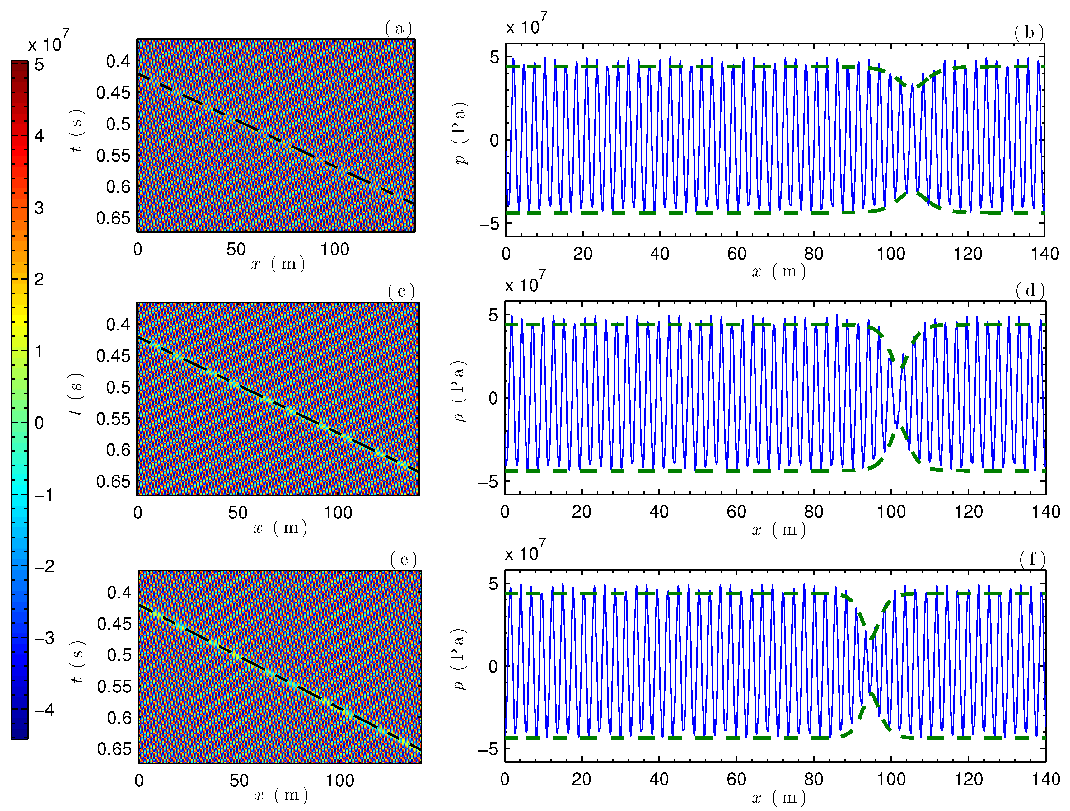
We now focus on the numerical study of the evolution of the gray soliton in the lattice. We start with the lossless case, by integrating Equation (3) with a driver of the form given by Equation (35) at $x=0$, with $ϵ=0.01$ ($2ϵ\eta P_0=4.39\times {10}^7$ Pa) and $f=1300$ Hz. The phase angle in the simulations is chosen as $\varphi =\pi /4$, $\varphi =\pi /8$ and $\varphi =-\pi /8$—see, respectively, Figure 6a–f. We observe that the gray solitons propagate at a constant velocity with a constant amplitude, width and minimum intensity, as shown in the contour plot in Figure 6a,c,e. The numerical spatial profiles calculated at $t=0.35$ s (blue lines) are in good agreement with the corresponding analytical ones, Equation (35) (green dashed lines), as shown in Figure 6b,d,f.

The phase angle $\varphi$ determines the minimum intensity and the velocity of the gray soliton ${\overrightarrow{v}}_{gray}$, as well as the group velocity, $v_g=v_b+v_s$. Upon changing $\varphi$ (from $\varphi =\pi /4$ to $\varphi =\pi /8$ ), we observe that the group velocity and the minimum intensity decrease (see Figure 6b,d). The change of sign of $\varphi$ (from $\varphi =\pi /8$ to $\varphi =-\pi /8$ ) does not affect the minimum intensity of the gray soliton, as shown in Figure 6d,f. For $\varphi =-\pi /8$, the gray soliton moves in a direction opposite to that of the background (see Equation (36)). Our analytical prediction of Equation (36), illustrated by black dashed lines in Figure 6a,c,e, is in full agreement with the numerical results.

3.4. Gray Solitons under Dissipation

According to the perturbation theory for dark solitons [33], the gray soliton of Equation (18) evolves as:

$$\begin{array}{c}A={\eta }_0\left\{b\tanh \left[{\eta }_{0}b\left(\sqrt{\left|\frac{q}{k_r^{{}^{″}}}\right|}{\tilde{\tau }}_1-aq{\eta }_0{\chi }_2\right.\right.\right.\hfill \\ \left.\left.\left.-\sqrt{\left|\frac{q}{k_r^{{}^{″}}}\right|}{t}_0\right)\right]+ia\right\}{e}^{-iq{\eta }_0^2{\chi }_2-i{\sigma }_0},\hfill \end{array}$$

(37)

where

$$a=a_{0}exp(-\mathsf{\Lambda }{\chi }_2),$$

(38)

$$b=b_{0}exp(-\mathsf{\Lambda }{\chi }_2).$$

(39)

The background amplitude $A={\eta }_0\sqrt{a^2+b^2}={\eta }_{0}exp(-\mathsf{\Lambda }{\chi }_2)$ decays exponentially with the same rate as in the black soliton case, Equation (30). The first-order correction term is given by:

$$t_0=\frac{a_0}{4b_0{\eta }_0}exp(-\mathsf{\Lambda }{\chi }_2)+\frac{3a_0}{4b_0{\eta }_0}exp\left(\mathsf{\Lambda }{\chi }_2\right)-\frac{a_0}{b_0{\eta }_0},$$

(40)

and ${\sigma }_0$ is an extra phase induced by the perturbation. In the original coordinates, x and t, the approximate form of the gray soliton reads:

$$\begin{array}{c}p(x,t)\approx 2ϵ{\eta }_0{P}_0{b}_0{e}^{\frac{-\mathsf{\Lambda }{ϵ}^2{\omega }_B}{c_0}x}\hfill \\ \times \tanh \left\{ϵ{\eta }_0{b}_0{e}^{\frac{-\mathsf{\Lambda }{ϵ}^2{\omega }_B}{c_0}x}\sqrt{\left|\frac{q}{k_r^{{}^{″}}}\right|}{\omega }_B\left[t-\frac{k_r^{\prime }}{c_0}x\right.\right.\hfill \\ -ϵa_0{e}^{-\mathsf{\Lambda }{ϵ}^2\frac{{\omega }_B}{c_0}x}{\eta }_0\frac{\sqrt{\left|q{k}_r^{{}^{″}}\right|}}{c_0}x\hfill \\ \left.\left.-\frac{1}{ϵ{\omega }_B}\left(\frac{a_0}{4b_0{\eta }_0}{e}^{-\mathsf{\Lambda }{ϵ}^2\frac{{\omega }_B}{c_0}x}+\frac{3a_0}{4b_0{\eta }_0}{e}^{\mathsf{\Lambda }{ϵ}^2\frac{{\omega }_B}{c_0}x}-\frac{a_0}{b_0{\eta }_0}\right)\right]\right\}\hfill \\ \times cos\left(\omega {\omega }_{B}t-\frac{k_r{\omega }_B}{c_0}x-q{ϵ}^2{\eta }_0^2\frac{{\omega }_B}{c_0}x-{ϵ}^2\frac{{\omega }_B}{c_0}{\sigma }_0\right)\hfill \\ -2ϵ{\eta }_0{P}_0{a}_0{e}^{\frac{-\mathsf{\Lambda }{ϵ}^2{\omega }_B}{c_0}x}\hfill \\ \times sin\left(\omega {\omega }_{B}t-\frac{k_r{\omega }_B}{c_0}x-q{ϵ}^2{\eta }_0^2\frac{{\omega }_B}{c_0}x-{ϵ}^2\frac{{\omega }_B}{c_0}{\sigma }_0\right),\hfill \end{array}$$

(41)

with the velocity

$$v_g={\left(\frac{k_r^{\prime }}{c_0}+ϵa_0{e}^{-\mathsf{\Lambda }{ϵ}^2\frac{{\omega }_B}{c_0}x}{\eta }_0\frac{\sqrt{\left|q{k}_r^{{}^{″}}\right|}}{c_0}\right)}^{-1}.$$

(42)

During gray soliton propagation, both the background amplitude and the minimum intensity decrease exponentially due to losses, while the width increases (see Equation (41)).

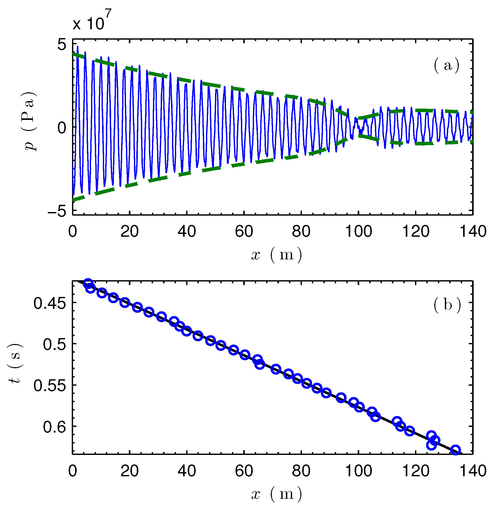
We numerically integrate the lattice model, Equation (3), with a gray soliton driver of the form given by Equation (35) or Equation (41), with $ϵ=0.01$ ($2ϵ\eta P_0=4.39\times {10}^7$ Pa) and $f=1300$ Hz. The numerical profile found at $t=0.58$ s, with $\varphi =\pi /8$, is shown in Figure 7a (blue line), is in a good agreement with the analytical prediction (green dashed line), Equation (41). The numerically obtained gray soliton trajectory [blue circles in Figure 7b], and is in good agreement with the analytical expression given in Equation (42).

4. Conclusions

In conclusion, we have theoretically and numerically studied envelope dark (black and gray) solitons in 1D nonlinear acoustic metamaterial composed of a waveguide with a periodic array of side holes, featuring viscothermal and radiation losses. Based on the electro-acoustic analogy and transmission line approach, we derived a nonlinear lattice model. We studied the linear dispersion relation of our system, which was found to be in good agreement with the one obtained by using the transfer matrix method. We used a multiple scale perturbation method to analytically treat the problem, and derived an effective NLS model describing the evolution of the pressure. We predicted the existence of dark solitons and studied analytically their evolution in the presence of losses. We investigated the interplay between dissipation, nonlinearity and dispersion, as described by pertinent characteristic length scales, in the case of a water-filled acoustic metamaterial with a small radius of side holes. The numerical results were found to be in good agreement with the analytical predictions.

Our results and methodology pave the way for studies on nonlinear phenomena in double-negative acoustic metamaterials, e.g., waveguides periodically loaded with side holes and clamped elastic plates. Our works will also help in designing new nonlinear acoustic metamaterials supporting bright, gap, black and grey solitons. According to the properties of the solitons, i.e., propagation with no distortion of high amplitude waves, our studies could also pave the way to designing new devices in medical applications or to designing non destructive sensors.

References

- Kivshar, Y.S.; Luther-Davies, B. Dark optical solitons: Physics and applications. Phys. Rep. 1998, 298, 81–197. [Google Scholar] [CrossRef]
- Frantzeskakis, D.J. Dark solitons in atomic Bose–Einstein condensates: From theory to experiments. J. Phys. A Math. Theor. 2010, 43, 213001. [Google Scholar] [CrossRef]
- Denardo, B.; Galvin, B.; Greenfield, A.; Larraza, A.; Putterman, S.; Wright, W. Observations of localized structures in nonlinear lattices: Domain walls and kinks. Phys. Rev. Lett. 1992, 68, 1730. [Google Scholar] [CrossRef] [PubMed]
- Chen, M.; Tsankov, M.A.; Nash, J.M.; Patton, C.E. Microwave magnetic-envelope dark solitons in yttrium iron garnet thin films. Phys. Rev. Lett. 1993, 70, 1707. [Google Scholar] [CrossRef] [PubMed]
- Heidemann, R.; Zhdanov, S.; Sütterlin, R.; Thomas, H.M.; Morfill, G.E. Dissipative dark soliton in a complex plasma. Phys. Rev. Lett. 2009, 102, 135002. [Google Scholar] [CrossRef] [PubMed]
- Chabchoub, A.; Kimmoun, O.; Branger, H.; Hoffmann, N.; Proment, D.; Onorato, M.; Akhmediev, N. Experimental observation of dark solitons on the surface of water. Phys. Rev. Lett. 2013, 110, 124101. [Google Scholar] [CrossRef] [PubMed]
- Sánchez-Morcillo, V.J.; Pérez-Arjona, I.; Romero-García, V.; Tournat, V.; Gusev, V.E. Second-harmonic generation for dispersive elastic waves in a discrete granular chain. Phys. Rev. E 2013, 88, 043203. [Google Scholar] [CrossRef] [PubMed]
- Jiménez, N.; Mehrem, A.; Picó, R.; García-Raffi, L.M.; Sánchez-Morcillo, V.J. Nonlinear propagation and control of acoustic waves in phononic superlattices. CR PHYS 2016, 17, 543–554. [Google Scholar] [CrossRef] [Green Version]
- Zhang, J.; Romero-García, V.; Theocharis, G.; Richoux, O.; Achilleos, V.; Frantzeskakis, D.J. Second-Harmonic Generation in Membrane-Type Nonlinear Acoustic Metamaterials. Crystals 2016, 6, 86. [Google Scholar] [CrossRef]
- Hamilton, M.; Blackstock, D.T. Nonlinear Acoustics; Academic Press: San Diego, CA, USA, 1998. [Google Scholar]
- Averkiou, M.A.; Lee, Y.S.; Hamilton, M.F. Self demodulation of amplitude and frequency modulated pulses in a thermoviscous fluid. J. Acoust. Soc. Am. 1993, 94, 2876–2883. [Google Scholar] [CrossRef]
- Achilleos, V.; Richoux, O.; Theocharis, G.; Frantzeskakis, D.J. Acoustic solitons in waveguides with Helmholtz resonators: Transmission line approach. Phys. Rev. E 2015, 91, 023204. [Google Scholar] [CrossRef] [PubMed]
- Sugimoto, N.; Masuda, M.; Ohno, J.; Motoi, D. Experimental demonstration of generation and propagation of acoustic solitary waves in an air-filled tube. Phys. Rev. Lett. 1999, 83, 4053. [Google Scholar] [CrossRef]
- Zhang, J.; Romero-García, V.; Theocharis, G.; Richoux, O.; Achilleos, V.; Frantzeskakis, D.J. Bright and Gap Solitons in Membrane-Type Acoustic Metamaterials. Phys. Rev. E 2017, 96, 022214. [Google Scholar] [CrossRef] [PubMed]
- Deng, B.; Raney, J.R.; Tournat, V.; Bertoldi, K. Elastic Vector Solitons in Soft Architected Materials. Phys. Rev. Lett. 2017, 118, 204102. [Google Scholar] [CrossRef] [PubMed]
- Singhal, T.; Kim, E.; Kim, T.; Yang, J. Weak bond detection in composites using highly nonlinear solitary waves. Smart Mater. Struct. 2017, 26, 055011. [Google Scholar] [CrossRef]
- Liu, Z.; Zhang, X.; Mao, Y.; Zhu, Y.Y.; Yang, Z.; Chan, C.T.; Sheng, P. Locally resonant sonic materials. Science 2000, 289, 1734–1736. [Google Scholar] [CrossRef] [PubMed]
- Fang, N.; Xi, D.; Xu, J.; Ambati, M.; Srituravanich, W.; Sun, C.; Zhang, X. Ultrasonic metamaterials with negative modulus. Nat. Mater. 2006, 5, 452. [Google Scholar] [CrossRef] [PubMed]
- Sugimoto, N.; Horioka, T. Dispersion characteristics of sound waves in a tunnel with an array of Helmholtz resonators. J. Acoust. Soc. Am. 1995, 97, 1446–1459. [Google Scholar] [CrossRef]
- Bradly, C.E. Time harmonic acoustic Bloch wave propagation in periodic waveguides. Part I. Theory. J. Acoust. Soc. Am. 1994, 96, 1844–1853. [Google Scholar] [CrossRef]
- Ma, G.; Yang, M.; Xiao, S.; Yang, Z.; Sheng, P. Acoustic metasurface with hybrid resonances. Nat. Mater. 2014, 13, 873–878. [Google Scholar] [CrossRef] [PubMed]
- Romero-García, V.; Theocharis, G.; Richoux, O.; Merkel, A.; Tournat, V.; Pagneux, V. Perfect and broadband acoustic absorption by critically coupled sub-wavelength resonators. Sci. Rep. 2016, 6, 19519. [Google Scholar] [CrossRef] [PubMed] [Green Version]
- Solymar, L.; Shamonina, E. Waves in Metamaterials; Oxford University Press: New York, NY, USA, 2009. [Google Scholar]
- Henríquez, V.C.; García-Chocano, V.M.; Sánchez-Dehesa, J. Viscothermal Losses in Double-Negative Acoustic Metamaterials. Phys. Rev. Appl. 2017, 8, 014029. [Google Scholar] [CrossRef]
- Zwikker, C.; Kosten, C.W. Sound Absorbing Materials; Elsevier: Amsterdam, The Netherland, 1949. [Google Scholar]
- Theocharis, G.; Richoux, O.; García, V.R.; Merkel, A.; Tournat, V. Limits of slow sound propagation and transparency in lossy, locally resonant periodic structures. New J. Phys. 2014, 16, 093017. [Google Scholar] [CrossRef] [Green Version]
- Bradley, C.E. Time harmonic acoustic Bloch wave propagation in periodic waveguides. Part II. Experiment. J. Acoust. Soc. Am. 1994, 96, 1854–1862. [Google Scholar] [CrossRef]
- Bongard, F.; Lissek, H.; Mosig, J.R. Acoustic transmission line metamaterial with negative/zero/positive refractive index. Phys. Rev. B 2010, 82, 094306. [Google Scholar] [CrossRef]
- Park, C.M.; Park, J.J.; Lee, S.H.; Seo, Y.M.; Kim, C.K.; Lee, S.H. Amplification of acoustic evanescent waves using metamaterial slabs. Phys. Rev. Lett. 2011, 107, 194301. [Google Scholar] [CrossRef] [PubMed]
- Lee, K.J.B.; Jung, M.K.; Lee, S.H. Highly tunable acoustic metamaterials based on a resonant tubular array. Phys. Rev. B 2012, 86, 184302. [Google Scholar] [CrossRef]
- Fleury, R.; Alú, A. Extraordinary sound transmission through density-near-zero ultranarrow channels. Phys. Rev. Lett. 2013, 111, 055501. [Google Scholar] [CrossRef] [PubMed]
- Rossing, T.D.; Fletcher, N.H. Principles of Vibration and Sound; Springer: New York, NY, USA, 1995. [Google Scholar]
- Ablowitz, M.J.; Nixon, S.D.; Horikis, T.P.; Frantzeskakis, D.J. Perturbations of dark solitons. Proc. R. Soc. A 2011, 467, 2597. [Google Scholar] [CrossRef]
- Atig, M.; Dalmont, J.P.; Gilbert, J. Termination impedance of open-ended cylindrical tubes at high sound pressure level. CR MECANIQUE 2004, 332, 299–304. [Google Scholar] [CrossRef]
- Buick, J.M.; Atig, M.; Skulina, D.J.; Campbell, D.M.; Dalmont, J.P.; Gilbert, J. Investigation of non- linear acoustic losses at the open end of a tube. J. Acoust. Soc. Am. 2011, 129, 1261–1272. [Google Scholar] [CrossRef] [PubMed] [Green Version]
- Kalozoumis, P.A.; Richoux, O.; Diakonos, F.K.; Theocharis, G.; Schmelcher, P. Invariant currents in lossy acoustic waveguides with complete local symmetry. Phys. Rev. B 2015, 92, 014303. [Google Scholar] [CrossRef]
- Dubos, V.; Kergomard, J.; Keefe, D.; Dalmont, J.-P.; Khettabi, A.; Nederveen, K. Theory of sound propagation in a duct with a branched tube using modal decomposition. Acta Acust. United Acust. 1999, 85, 153–169. [Google Scholar]
- Dalmont, J.-P.; Nederveen, C.J.; Joly, N. Radiation impedance of tubes with different flanges: Numerical and experimental investigations. J. Sound Vib. 2001, 244, 505–534. [Google Scholar] [CrossRef]
- Remoissenet, M. Waves Called Solitons; Springer: Berlin, Germany, 1999. [Google Scholar]
- Ablowitz, M.J. Nonlinear Dispersive Waves, Asymptotic Analysis and Solitons; Cambridge University Press: Cambridge, UK, 2011. [Google Scholar]
Figure 1.
(color online) (a) waveguide loaded with an array of side holes; (b) corresponding unit-cell circuit.
Figure 2.
(color online) (a,b) show the real and imaginary parts of the complex dispersion relation respectively. The blue circles (green stars) show the results from the TL (TMM) approach from Equation (10) [Equation (11)]; the blue dashed (green continuous) lines show the lossless dispersion relation obtained from the TL (TMM) approach from the lossless limit of Equation (10) (Equation (11)); (c) the frequency dependent , the product of the nonlinearity and the dispersion coefficients of NLS equations.
Figure 3.
(color online) (a) a contour plot of black soliton of the form of Equation (25), obtained by numerically integrating the lossless version of Equation (3) () with ( Pa) (170 dB) and carrier frequency Hz; (b) numerical spatial profile of black soliton calculated at s (blue line). Green dashed lines are the corresponding analytical envelope result of Equation (25). The light green thick line denotes the nonlinear length and dispersion length , with m; (c) a numerical contour plot for dispersive effect, obtained by numerically integrating the lossless version of Equation (3) (). Keeping the same width, we only decrease the amplitude of the driver to ( Pa) (160 dB) such as the nonlinearity can not balance the dispersion; (d) numerical spatial profile of dispersive wave calculated at s.
Figure 4.
(color online) Effects of radiation and viscothermal losses on black soliton propagation in an air-filled acoustic metamaterial with m, m, m, , calculated at s. Numerical dissipative black soliton (blue line) is obtained by integrating our lattice model Equation (3) with the driver corresponding to ( Pa) (170 dB) and Hz, Equation (25) or Equation (33). The green dashed line is the corresponding analytical envelope result, Equation (33). The light green thick line denotes the nonlinear length and dispersion length , with m.
Figure 5.
(color online) Effects of radiation and viscothermal losses on black soliton propagation in an water-filled acoustic metamaterial with m, m, m, m, calculated at (a) s; (b) s and (c) s, respectively. A numerical dissipative black soliton (blue line) is obtained by integrating the lattice model Equation (3) with the driver corresponding to ( Pa) and Hz. Green dashed line is the corresponding analytical envelope results, Equation (33). The light green thick line denotes the nonlinear length and dispersion length , with m.
Figure 6.
(color online) (a) a contour plot of gray soliton of the form of Equation (35), obtained by numerically integrating the lossless lattice model of Equation (3) (), with , ( Pa) and Hz; (b) numerical spatial profile of gray soliton calculated at s with (blue line); (c) contour plot of gray soliton with ; (d) numerical spatial profile of gray soliton calculated at s with (blue line); (e) contour plot of gray soliton with ; (f) numerical spatial profile of gray soliton calculated at s with (blue line). Black dashed lines in (a,c,e), presenting the information about the velocity of the gray solitons, are the corresponding analytical results, Equation (36). Green dashed lines in (b,d,f) stand for the corresponding analytical envelopes of gray solitons.
Figure 7.
(color online) (a) numerical spatial profile of dissipative gray soliton calculated at s with (blue line). Green dashed lines are the corresponding analytical envelope, Equation (41); (b) the corresponding space-time diagram of dissipative gray soliton (blue circles). The slope of the black line shows the analytical velocity of dissipative gray solitons, Equation (42).
© 2018 by the authors. Licensee MDPI, Basel, Switzerland. This article is an open access article distributed under the terms and conditions of the Creative Commons Attribution (CC BY) license (http://creativecommons.org/licenses/by/4.0/).
Share and Cite
MDPI and ACS Style
Zhang, J.; Romero-García, V.; Theocharis, G.; Richoux, O.; Achilleos, V.; Frantzeskakis, D.J. Dark Solitons in Acoustic Transmission Line Metamaterials. Appl. Sci. 2018, 8, 1186. https://doi.org/10.3390/app8071186
AMA Style
Zhang J, Romero-García V, Theocharis G, Richoux O, Achilleos V, Frantzeskakis DJ. Dark Solitons in Acoustic Transmission Line Metamaterials. Applied Sciences. 2018; 8(7):1186. https://doi.org/10.3390/app8071186
Chicago/Turabian StyleZhang, Jiangyi, Vicente Romero-García, Georgios Theocharis, Olivier Richoux, Vassos Achilleos, and Dimitrios J. Frantzeskakis. 2018. "Dark Solitons in Acoustic Transmission Line Metamaterials" Applied Sciences 8, no. 7: 1186. https://doi.org/10.3390/app8071186
Note that from the first issue of 2016, this journal uses article numbers instead of page numbers. See further details here.