Spatial Modelling of Gully Erosion Using GIS and R Programing: A Comparison among Three Data Mining Algorithms

 ,
,  ,
,  ,
,
Abstract
:
1. Introduction
2. Materials and Methods
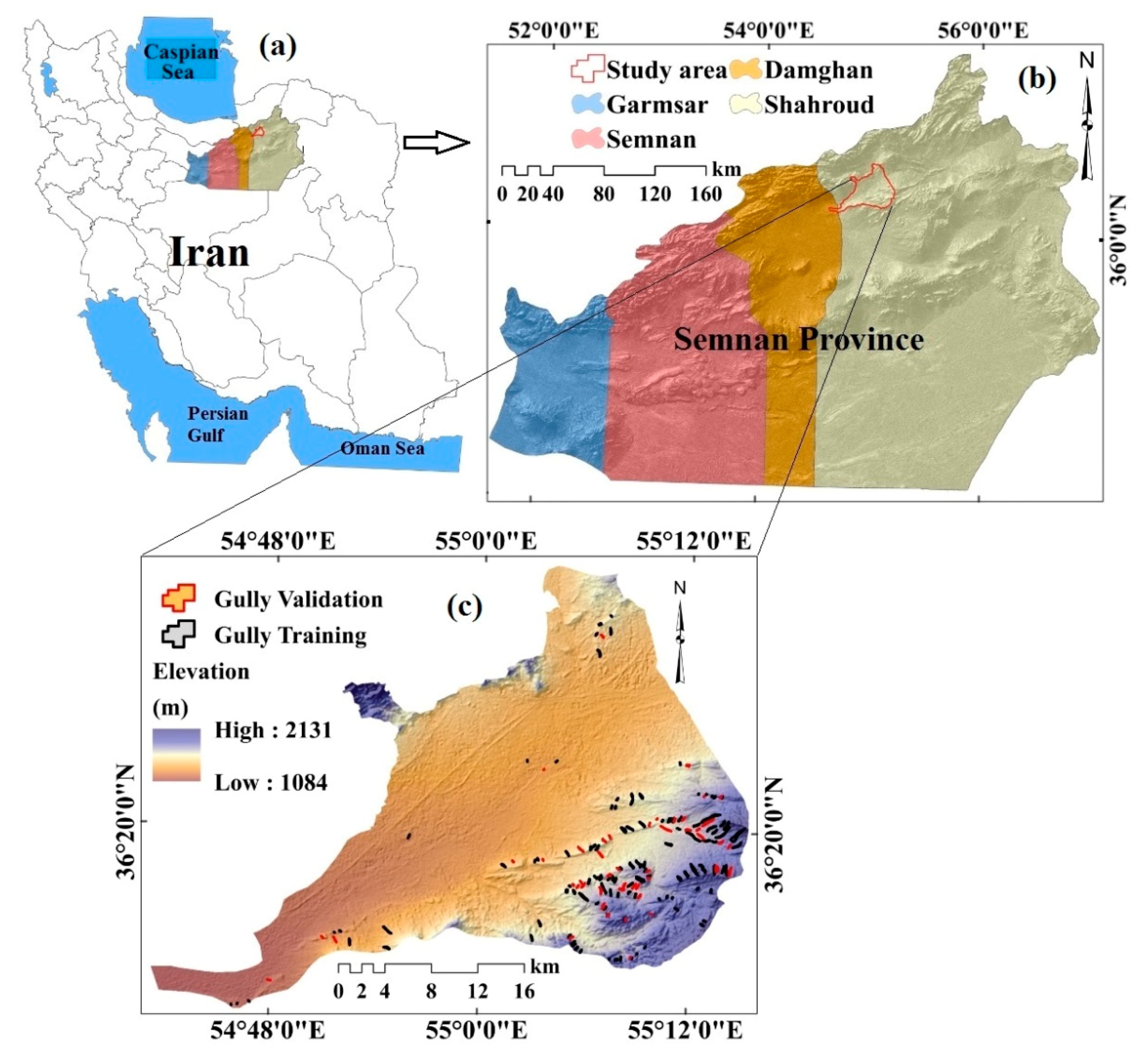
2.1. Study Area
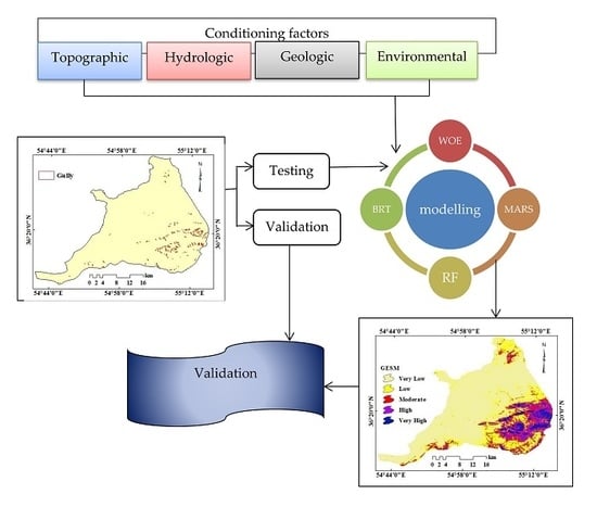
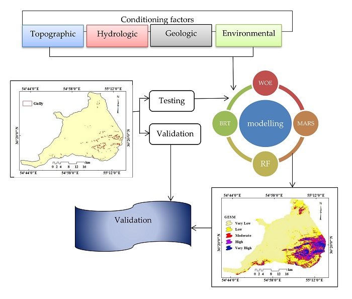
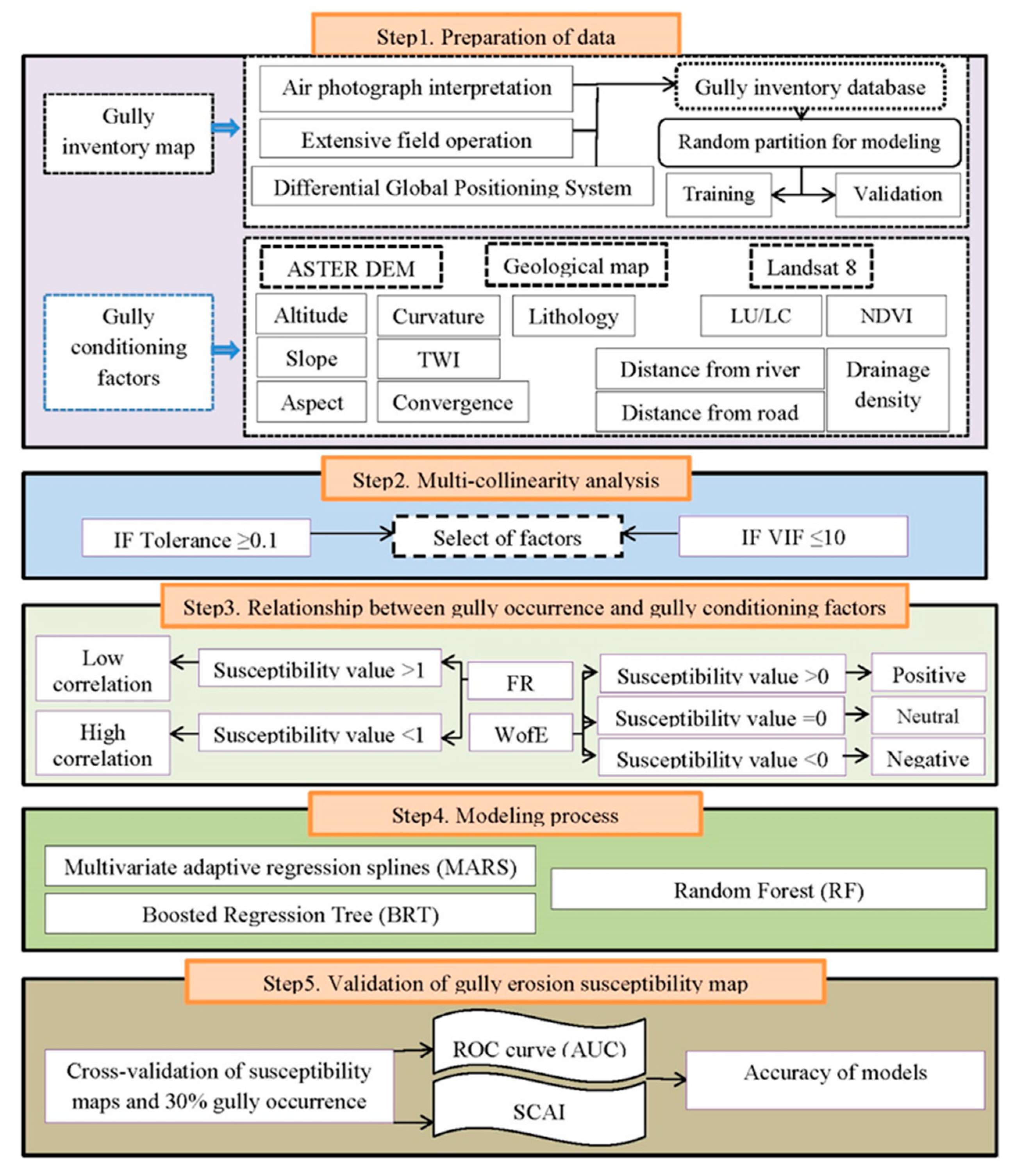
2.2. Data and Method
2.3. Gully Erosion Modelling
2.3.1. WoE Model
2.3.2. RF Model
2.3.3. BRT Model
2.3.4. MARS Model
2.4. Validation of GESMs Using Three Data Mining Models
3. Results
3.1. Multi-Collinearity Analysis
3.2. Spatial Relationship Using WoE Model
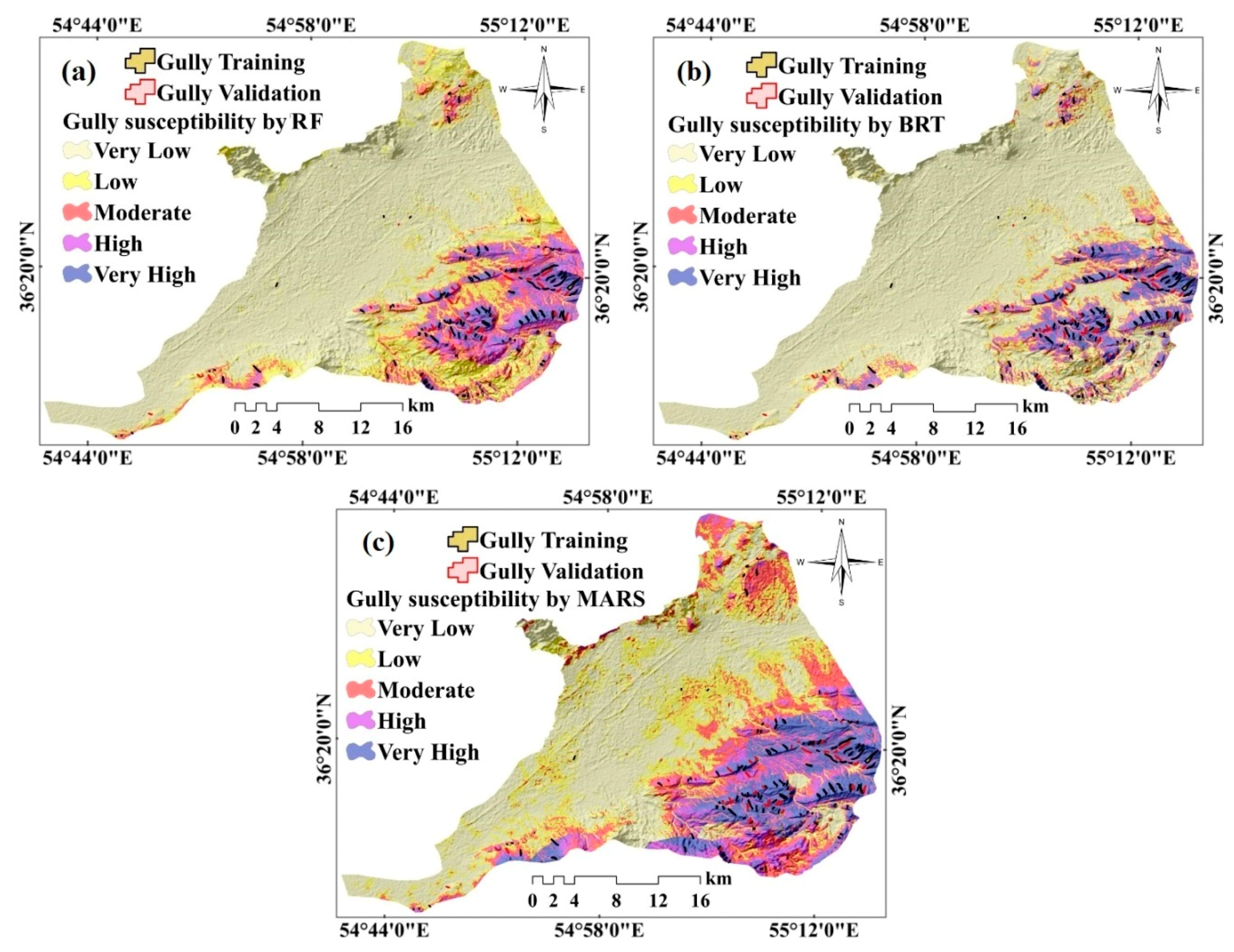
3.3. Applying RF Model
3.4. Applying BRT Model
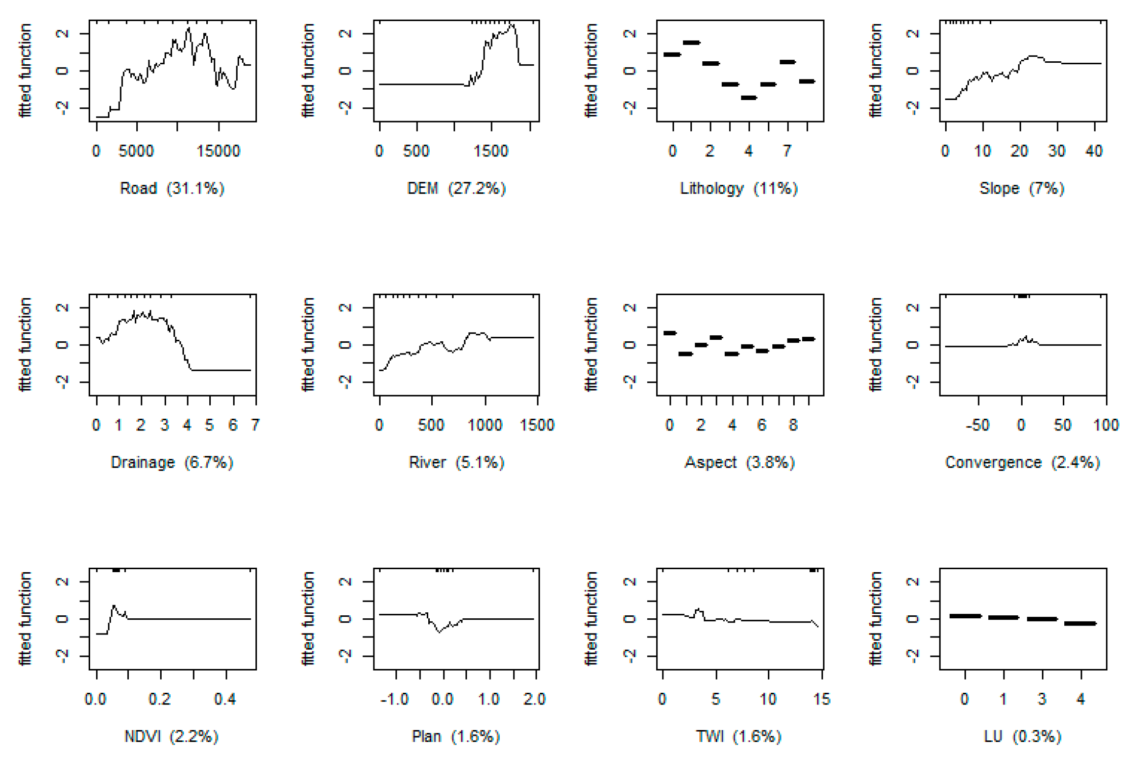
3.5. Applying MARS Model
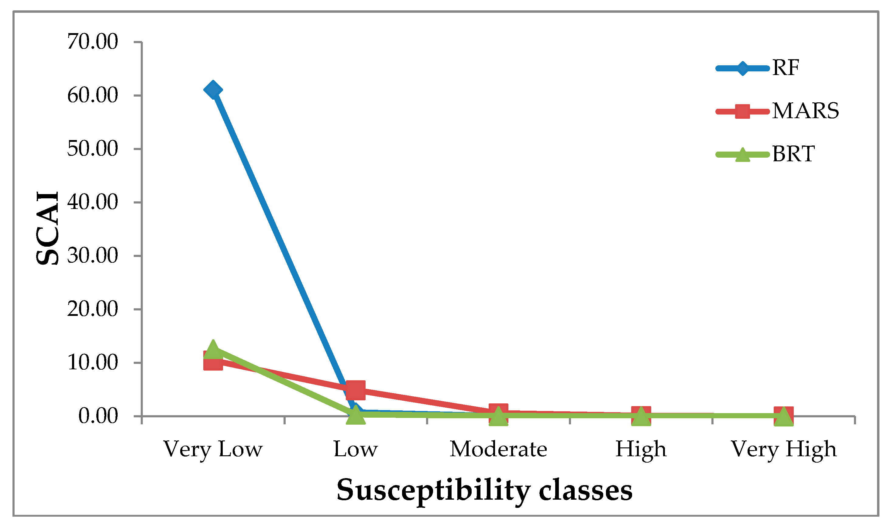
3.6. Validation of Models
4. Discussion
5. Conclusions
Author Contributions
Funding
Conflicts of Interest
References
- Magliulo, P. Assessing the susceptibility to water-induced soil erosion using a geomorphological, bivariate statistics-based approach. Environ. Earth Sci. 2012, 67, 1801–1820. [Google Scholar] [CrossRef]
- UNEP. The Emissions Gap Report. United Nations Environment Programme (UNEP). Nairobi, 2017. Available online: www.unenvironment.org/resources/emissions-gap-report (accessed on 13 January 2018).
- Haregeweyn, N.; Tsunekawa, A.; Poesen, J.; Tsubo, M.; Meshesha, D.T.; Fenta, A.A.; Nyssen, J.; Adgo, E. Comprehensive assessment of soil erosion risk for better land use planning in river basins: Case study of the Upper Blue Nile River. Sci. Total Environ. 2017, 574, 95–108. [Google Scholar] [CrossRef] [PubMed]
- Nampak, H.; Pradhan, B.; Mojaddadi Rizeei, H.; Park, H.-J. Assessment of Land Cover and Land Use Change Impact on Soil Loss in a Tropical Catchment by Using Multi-Temporal SPOT-5 Satellite Images and RUSLE model. Land Degrad. Dev. 2018. [Google Scholar] [CrossRef]
- Rizeei, H.M.; Saharkhiz, M.A.; Pradhan, B.; Ahmad, N. Soil erosion prediction based on land cover dynamics at the Semenyih watershed in Malaysia using LTM and USLE models. Geocarto Int. 2016, 31, 1158–1177. [Google Scholar] [CrossRef]
- Zhang, X.; Fan, J.; Liu, Q.; Xiong, D. The contribution of gully erosion to total sediment production in a small watershed in Southwest China. Phys. Geogr. 2018, 39, 246–263. [Google Scholar] [CrossRef]
- Mojaddadi, H.; Habibnejad, M.; Solaimani, K.; Ahmadi, M.; Hadian-Amri, M. An Investigation of Efficiency of Outlet Runoff Assessment. J. Appl. Sci. 2009, 9, 105–112. [Google Scholar]
- Zabihi, M.; Mirchooli, F.; Motevalli, A.; Darvishan, A.K.; Pourghasemi, H.R.; Zakeri, M.A.; Sadighi, F. Spatial modelling of gully erosion in Mazandaran Province, northern Iran. Catena 2018, 161, 1–13. [Google Scholar] [CrossRef]
- Kirkby, M.; Bracken, L. Gully processes and gully dynamics. Earth Surf. Process. Landf. J. Br. Geomorphol. Res. Group 2009, 34, 1841–1851. [Google Scholar] [CrossRef]
- Torri, D.; Poesen, J.; Borselli, L.; Bryan, R.; Rossi, M. Spatial variation of bed roughness in eroding rills and gullies. Catena 2012, 90, 76–86. [Google Scholar] [CrossRef]
- Mccloskey, G.; Wasson, R.; Boggs, G.; Douglas, M. Timing and causes of gully erosion in the riparian zone of the semi-arid tropical Victoria River, Australia: Management implications. Geomorphology 2016, 266, 96–104. [Google Scholar] [CrossRef]
- Rahmati, O.; Tahmasebipour, N.; Haghizadeh, A.; Pourghasemi, H.R.; Feizizadeh, B. Evaluating the influence of geo-environmental factors on gully erosion in a semi-arid region of Iran: An integrated framework. Sci. Total Environ. 2017, 579, 913–927. [Google Scholar] [CrossRef] [PubMed]
- Dube, F.; Nhapi, I.; Murwira, A.; Gumindoga, W.; Goldin, J.; Mashauri, D. Potential of weight of evidence modelling for gully erosion hazard assessment in Mbire District–Zimbabwe. Phys. Chem. Earth Part A/B/C 2014, 67, 145–152. [Google Scholar] [CrossRef]
- Zakerinejad, R.; Maerker, M. An integrated assessment of soil erosion dynamics with special emphasis on gully erosion in the Mazayjan basin, southwestern Iran. Nat. Hazards 2015, 79, 25–50. [Google Scholar] [CrossRef]
- Pham, T.G.; Degener, J.; Kappas, M. Integrated universal soil loss equation (USLE) and Geographical Information System (GIS) for soil erosion estimation in A Sap basin: Central Vietnam. Int. Soil Water Conserv. Res. 2018, 6, 99–110. [Google Scholar] [CrossRef]
- Pournader, M.; Ahmadi, H.; Feiznia, S.; Karimi, H.; Peirovan, H.R. Spatial prediction of soil erosion susceptibility: An evaluation of the maximum entropy model. Earth Sci. Inform. 2018, 11, 389–401. [Google Scholar] [CrossRef]
- Althuwaynee, O.F.; Pradhan, B.; Park, H.-J.; Lee, J.H. A novel ensemble bivariate statistical evidential belief function with knowledge-based analytical hierarchy process and multivariate statistical logistic regression for landslide susceptibility mapping. Catena 2014, 114, 21–36. [Google Scholar] [CrossRef]
- Morgan, R.; Quinton, J.; Smith, R.; Govers, G.; Poesen, J.; Auerswald, K.; Chisci, G.; Torri, D.; Styczen, M. The European Soil Erosion Model (EUROSEM): A dynamic approach for predicting sediment transport from fields and small catchments. Earth Surf. Process. Landf. J. Br. Geomorphol. Res. Group 1998, 23, 527–544. [Google Scholar] [CrossRef]
- Barber, M.; Mahler, R. Ephemeral gully erosion from agricultural regions in the Pacific Northwest, USA. Ann. Wars. Univ. Life Sci.-SGGW. Land Reclam. 2010, 42, 23–29. [Google Scholar] [CrossRef] [Green Version]
- Leonard, R.; Knisel, W.; Still, D. GLEAMS: Groundwater loading effects of agricultural management systems. Trans. ASAE 1987, 30, 1403–1418. [Google Scholar] [CrossRef]
- Liaw, A.; Breiman, W.M. Cutler’s Random Forests for Classification and Regression. Available online: https://www.rdocumentation.org/packages/randomForest (accessed on 1 April 2018).
- Akgün, A.; Türk, N. Mapping erosion susceptibility by a multivariate statistical method: A case study from the Ayvalık region, NW Turkey. Comput. Geosci. 2011, 37, 1515–1524. [Google Scholar] [CrossRef]
- Conoscenti, C.; Angileri, S.; Cappadonia, C.; Rotigliano, E.; Agnesi, V.; Märker, M. Gully erosion susceptibility assessment by means of GIS-based logistic regression: A case of Sicily (Italy). Geomorphology 2014, 204, 399–411. [Google Scholar] [CrossRef] [Green Version]
- Conforti, M.; Aucelli, P.P.; Robustelli, G.; Scarciglia, F. Geomorphology and GIS analysis for mapping gully erosion susceptibility in the Turbolo stream catchment (Northern Calabria, Italy). Nat. Hazards 2011, 56, 881–898. [Google Scholar] [CrossRef]
- Lucà, F.; Conforti, M.; Robustelli, G. Comparison of GIS-based gullying susceptibility mapping using bivariate and multivariate statistics: Northern Calabria, South Italy. Geomorphology 2011, 134, 297–308. [Google Scholar] [CrossRef]
- Meyer, A.; Martınez-Casasnovas, J. Prediction of existing gully erosion in vineyard parcels of the NE Spain: A logistic modelling approach. Soil Tillage Res. 1999, 50, 319–331. [Google Scholar] [CrossRef]
- Kuhnert, P.M.; Henderson, A.K.; Bartley, R.; Herr, A. Incorporating uncertainty in gully erosion calculations using the random forests modelling approach. Environmetrics 2010, 21, 493–509. [Google Scholar] [CrossRef]
- Rahmati, O.; Haghizadeh, A.; Pourghasemi, H.R.; Noormohamadi, F. Gully erosion susceptibility mapping: The role of GIS-based bivariate statistical models and their comparison. Nat. Hazards 2016, 82, 1231–1258. [Google Scholar] [CrossRef]
- Svoray, T.; Michailov, E.; Cohen, A.; Rokah, L.; Sturm, A. Predicting gully initiation: Comparing data mining techniques, analytical hierarchy processes and the topographic threshold. Earth Surf. Proc. Land. 2012, 37, 607–619. [Google Scholar] [CrossRef]
- Zakerinejad, R.; Märker, M. Prediction of Gully erosion susceptibilities using detailed terrain analysis and maximum entropy modeling: A case study in the Mazayejan Plain, Southwest Iran. Geogr. Fis. Din. Quat. 2014, 37, 67–76. [Google Scholar]
- Pourghasemi, H.R.; Yousefi, S.; Kornejady, A.; Cerdà, A. Performance assessment of individual and ensemble data-mining techniques for gully erosion modeling. Sci. Total Environ. 2017, 609, 764–775. [Google Scholar] [CrossRef] [PubMed] [Green Version]
- I.R. of Iran Meteorological Organization. 2012. Available online: http://www.mazan daranmet.ir/ (accessed on 12 October 2017).
- Geological Survey Department of Iran (GSDI). 2012. Available online: http://www.mazan daranmet.ir/ (accessed on 12 October 2017).
- Althuwaynee, O.F.; Pradhan, B.; Lee, S. Application of an evidential belief function model in landslide susceptibility mapping. Comput. Geosci. 2012, 44, 120–135. [Google Scholar] [CrossRef]
- Rizeei, H.M.; Pradhan, B.; Saharkhiz, M.A. Surface runoff prediction regarding LULC and climate dynamics using coupled LTM, optimized ARIMA, and GIS-based SCS-CN models in tropical region. Arab. J. Geosci. 2018, 11, 53. [Google Scholar] [CrossRef]
- Chen, W.; Xie, X.; Wang, J.; Pradhan, B.; Hong, H.; Bui, D.T.; Duan, Z.; Ma, J. A comparative study of logistic model tree, random forest, and classification and regression tree models for spatial prediction of landslide susceptibility. Catena 2017, 151, 147–160. [Google Scholar] [CrossRef]
- Tehrany, M.S.; Pradhan, B.; Mansor, S.; Ahmad, N. Flood susceptibility assessment using GIS-based support vector machine model with different kernel types. Catena 2015, 125, 91–101. [Google Scholar] [CrossRef]
- Claps, P.; Fiorentino, M.; Oliveto, G. Informational entropy of fractal river networks. J. Hydrol. 1996, 187, 145–156. [Google Scholar] [CrossRef] [Green Version]
- Aal-Shamkhi, A.D.S.; Mojaddadi, H.; Pradhan, B.; Abdullahi, S. Extraction and modeling of urban sprawl development in Karbala City using VHR satellite imagery. In Spatial Modeling and Assessment of Urban Form; Springer: Berlin, Germany, 2017; pp. 281–296. [Google Scholar]
- Abdullahi, S.; Pradhan, B.; Mojaddadi, H. City compactness: Assessing the influence of the growth of residential land use. J. Urban Technol. 2018, 25, 21–46. [Google Scholar] [CrossRef]
- Rizeei, H.M.; Shafri, H.Z.; Mohamoud, M.A.; Pradhan, B.; Kalantar, B. Oil palm counting and age estimation from WorldView-3 imagery and LiDAR data using an integrated OBIA height model and regression analysis. J. Sensors 2018, 2018, 2536327. [Google Scholar] [CrossRef]
- Xie, Z.; Chen, G.; Meng, X.; Zhang, Y.; Qiao, L.; Tan, L. A comparative study of landslide susceptibility mapping using weight of evidence, logistic regression and support vector machine and evaluated by SBAS-InSAR monitoring: Zhouqu to Wudu segment in Bailong River Basin, China. Environ. Earth Sci. 2017, 76, 313. [Google Scholar] [CrossRef]
- Lee, S.; Kim, J.-C.; Jung, H.-S.; Lee, M.J.; Lee, S. Spatial prediction of flood susceptibility using random-forest and boosted-tree models in Seoul metropolitan city, Korea. Geomat. Nat. Hazards Risk 2017, 8, 1185–1203. [Google Scholar] [CrossRef]
- Cutler, D.R.; Edwards Jr, T.C.; Beard, K.H.; Cutler, A.; Hess, K.T.; Gibson, J.; Lawler, J.J. Random forests for classification in ecology. Ecology 2007, 88, 2783–2792. [Google Scholar] [CrossRef] [PubMed]
- Simpson, G.L.; Birks, H.J.B. Statistical learning in palaeolimnology. In Tracking Environmental Change Using Lake Sediments; Springer: Berlin, Germany, 2012; pp. 249–327. [Google Scholar]
- Nicodemus, K.K. Letter to the editor: On the stability and ranking of predictors from random forest variable importance measures. Brief. Bioinform. 2011, 12, 369–373. [Google Scholar] [CrossRef] [PubMed]
- Bui, D.T.; Bui, Q.-T.; Nguyen, Q.-P.; Pradhan, B.; Nampak, H.; Trinh, P.T. A hybrid artificial intelligence approach using GIS-based neural-fuzzy inference system and particle swarm optimization for forest fire susceptibility modeling at a tropical area. Agr. For. Meteorol. 2017, 233, 32–44. [Google Scholar]
- Elith, J.; Leathwick, J.R.; Hastie, T. A working guide to boosted regression trees. J. Anim. Ecol. 2008, 77, 802–813. [Google Scholar] [CrossRef] [PubMed] [Green Version]
- Regmi, A.D.; Devkota, K.C.; Yoshida, K.; Pradhan, B.; Pourghasemi, H.R.; Kumamoto, T.; Akgun, A. Application of frequency ratio, statistical index, and weights-of-evidence models and their comparison in landslide susceptibility mapping in Central Nepal Himalaya. Arab. J. Geosci. 2014, 7, 725–742. [Google Scholar] [CrossRef]
- Aertsen, W.; Kint, V.; Van Orshoven, J.; Özkan, K.; Muys, B. Comparison and ranking of different modelling techniques for prediction of site index in Mediterranean mountain forests. Ecol. Model. 2010, 221, 1119–1130. [Google Scholar] [CrossRef]
- Krishnaiah, V.; Narsimha, G.; Chandra, N.S. Heart disease prediction system using data mining techniques and intelligent fuzzy approach: A review. Heart Dis. 2016, 136, 43–51. [Google Scholar] [CrossRef]
- Oh, H.-J.; Pradhan, B. Application of a neuro-fuzzy model to landslide-susceptibility mapping for shallow landslides in a tropical hilly area. Comput. Geosci. 2011, 37, 1264–1276. [Google Scholar] [CrossRef]
- Torgo, L. Data Mining with R: Learning with Case Studies; Chapman and Hall/CRC: Boca Raton, FL, USA, 2016. [Google Scholar]
- Umar, Z.; Pradhan, B.; Ahmad, A.; Jebur, M.N.; Tehrany, M.S. Earthquake induced landslide susceptibility mapping using an integrated ensemble frequency ratio and logistic regression models in West Sumatera Province, Indonesia. Catena 2014, 118, 124–135. [Google Scholar] [CrossRef]
- Mojaddadi, H.; Pradhan, B.; Nampak, H.; Ahmad, N.; Ghazali, A.H.B. Ensemble machine-learning-based geospatial approach for flood risk assessment using multi-sensor remote-sensing data and GIS. Geomat. Nat. Hazards Risk 2017, 8, 1080–1102. [Google Scholar] [CrossRef]
- Pourghasemi, H.R.; Beheshtirad, M.; Pradhan, B. A comparative assessment of prediction capabilities of modified analytical hierarchy process (M-AHP) and Mamdani fuzzy logic models using Netcad-GIS for forest fire susceptibility mapping. Geomat. Nat. Hazards Risk 2016, 7, 861–885. [Google Scholar] [CrossRef]
- Hong, H.; Naghibi, S.A.; Dashtpagerdi, M.M.; Pourghasemi, H.R.; Chen, W. A comparative assessment between linear and quadratic discriminant analyses (LDA-QDA) with frequency ratio and weights-of-evidence models for forest fire susceptibility mapping in China. Arab. J. Geosci. 2017, 10, 167. [Google Scholar] [CrossRef]
- Mezaal, M.R.; Pradhan, B.; Shafri, H.; Mojaddadi, H.; Yusoff, Z. Optimized Hierarchical Rule-Based Classification for Differentiating Shallow and Deep-Seated Landslide Using High-Resolution LiDAR Data. In Global Civil Engineering Conference; Springer: Berlin, Germany, 2017. [Google Scholar]
- Rizeei, H.M.; Pradhan, B.; Saharkhiz, M.A. An integrated fluvial and flash pluvial model using 2D high-resolution sub-grid and particle swarm optimization-based random forest approaches in GIS. Complex Intell. Syst. 2018, 1–20. [Google Scholar] [CrossRef]
- Kantardzic, M. Data mining: Concepts, Models, Methods, and Algorithms; John Wiley & Sons: Hoboken, NJ, USA, 2011. [Google Scholar]
- Pham, B.T.; Pradhan, B.; Bui, D.T.; Prakash, I.; Dholakia, M. A comparative study of different machine learning methods for landslide susceptibility assessment: A case study of Uttarakhand area (India). Environ. Model. Softw. 2016, 84, 240–250. [Google Scholar] [CrossRef]
- Lai, C.; Chen, X.; Wang, Z.; Xu, C.-Y.; Yang, B. Rainfall-induced landslide susceptibility assessment using random forest weight at basin scale. Hydrol. Res. 2017, nh2017044. [Google Scholar] [CrossRef]


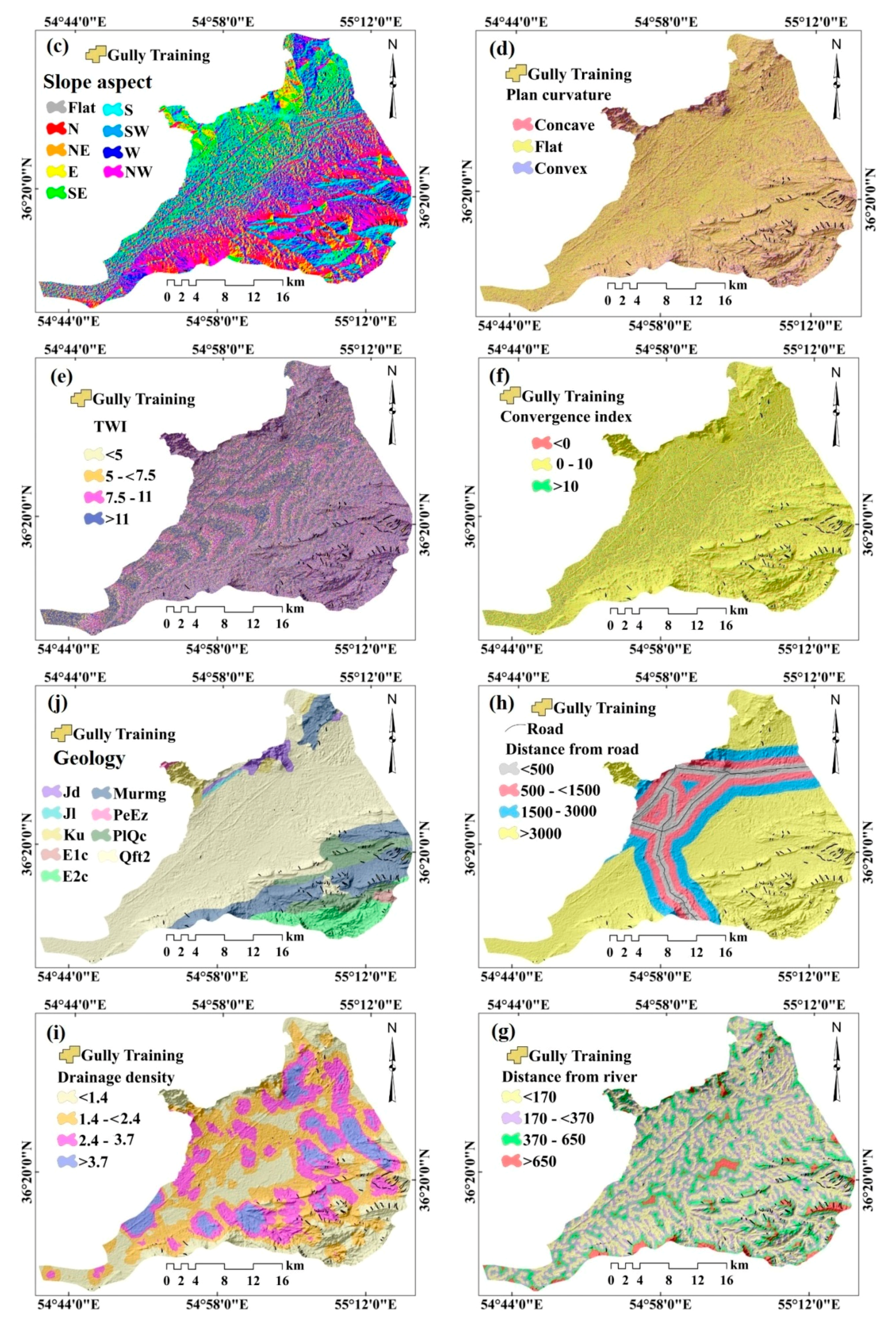
| Code | Lithology | Geological Age |
|---|---|---|
| Murmg | Gypsiferous marl | Miocene |
| Qft2 | Low level piedment fan and vally terrace deposits | Quaternary |
| Ku | Upper cretaceous, undifferentiated rocks | Cretaceous |
| Jd | Well—bedded to thin—bedded, greenish—grey argillaceous limestone with intercalations of calcareous shale (DALICHAI FM) | Jurassic |
| PeEz | Reef-type limestone and gypsiferous marl (ZIARAT FM) | Paleocene-Eocene |
| PlQc | Fluvial conglomerate, Piedmont conglomerate and sandstone. | Pliocene-Quaternary |
| Jl | Light grey, thin—bedded to massive limestone (LAR FM) | Jurassic-Cretaceous |
| E2c | Conglomerate and sandstone | Eocene |
| PlQc | Fluvial conglomerate, Piedmont conglomerate and sandstone. | Pliocene-Quaternary |
| E1c | Pale-red, polygenic conglomerate and sandstone | Paleocene-Eocene |
| Conditioning Factors | Collinearity Statistics | |
|---|---|---|
| Tolerance | VIF | |
| Constant Coefficient | - | - |
| Slope degree | 0.998 | 1.002 |
| Distance from road | 0.672 | 1.489 |
| Distance from river | 0.323 | 3.094 |
| Plan curvature | 0.674 | 1.483 |
| Lithology | 0.945 | 1.058 |
| LU | 0.864 | 1.158 |
| Drainage density | 0.826 | 1.211 |
| Elevation | 0.920 | 1.087 |
| Convergence index | 0.666 | 1.503 |
| Aspect | 0.299 | 3.343 |
| TWI | 0.942 | 1.062 |
| NDVI | 0.941 | 1.063 |
| Factor | Class | Number of Pixels in Domain | Pixels of Gullies | Weights-of-Evidence (WoE) | ||||
|---|---|---|---|---|---|---|---|---|
| C | S2 (w+) | S2 (w−) | S | W | ||||
| 1 | <1200 | 144,200 | 21 | −3.16 | 0.05 | 0.00 | 0.22 | −14.41 |
| 1200–<1350 | 348,463 | 89 | −2.87 | 0.01 | 0.00 | 0.11 | −26.60 | |
| 1350–<1450 | 230,735 | 502 | −0.37 | 0.00 | 0.00 | 0.05 | −7.52 | |
| 1450–1600 | 133,305 | 1057 | 0.33 | 0.00 | 0.00 | 0.00 | 0.00 | |
| >1600 | 85,376 | 1074 | 1.88 | 0.00 | 0.00 | 0.04 | 47.95 | |
| 2 | <5 | 705,163 | 896 | −1.83 | 0.00 | 0.00 | 0.04 | −44.90 |
| 5–<10 | 171,923 | 1259 | 1.34 | 0.00 | 0.00 | 0.04 | 34.96 | |
| 10–<15 | 38,854 | 397 | 1.38 | 0.00 | 0.00 | 0.05 | 25.36 | |
| 15–<20 | 13,936 | 121 | 1.13 | 0.01 | 0.00 | 0.09 | 12.13 | |
| 20–<25 | 6223 | 50 | 1.03 | 0.02 | 0.00 | 0.14 | 7.22 | |
| 25–30 | 3396 | 15 | 0.42 | 0.07 | 0.00 | 0.26 | 1.62 | |
| >30 | 2584 | 5 | −0.41 | 0.20 | 0.00 | 0.45 | −0.92 | |
| 3 | Flat | 16,770 | 2 | −3.22 | 0.50 | 0.00 | 0.71 | −4.55 |
| N | 72,345 | 208 | −0.01 | 0.00 | 0.00 | 0.07 | −0.19 | |
| NE | 79,383 | 209 | −0.11 | 0.00 | 0.00 | 0.07 | −1.52 | |
| E | 72,794 | 43 | −1.66 | 0.02 | 0.00 | 0.15 | −10.81 | |
| SE | 91,567 | 54 | −1.68 | 0.02 | 0.00 | 0.14 | −12.24 | |
| S | 114,731 | 246 | −0.34 | 0.00 | 0.00 | 0.07 | −5.13 | |
| SW | 119,263 | 396 | 0.15 | 0.00 | 0.00 | 0.05 | 2.81 | |
| W | 142,533 | 459 | 0.12 | 0.00 | 0.00 | 0.05 | 2.35 | |
| NW | 232,693 | 1126 | 0.76 | 0.00 | 0.00 | 0.04 | 19.46 | |
| 4 | Concave | 54,613 | 1493 | 2.99 | 0.00 | 0.00 | 0.04 | 78.04 |
| Flat | 574,180 | 749 | −1.43 | 0.00 | 0.00 | 0.04 | −33.33 | |
| Convex | 313,286 | 501 | −0.80 | 0.00 | 0.00 | 0.05 | −16.27 | |
| 5 | <7 | 24,272 | 63 | 0.00 | 0.00 | 0.00 | 0.02 | −0.15 |
| 5–<7.5 | 42,453 | 91 | −0.32 | 0.01 | 0.00 | 0.11 | −3.00 | |
| 7.5–11 | 89,328 | 225 | −0.16 | 0.00 | 0.00 | 0.07 | −2.29 | |
| >11 | 786,026 | 2364 | 0.21 | 0.00 | 0.00 | 0.06 | 3.87 | |
| 6 | <0 | 75,370 | 26 | −2.21 | 0.04 | 0.00 | 0.20 | −11.21 |
| 0–10 | 776,920 | 2534 | 0.95 | 0.00 | 0.00 | 0.07 | 13.18 | |
| >10 | 89,789 | 183 | −0.39 | 0.01 | 0.00 | 0.08 | −5.08 | |
| 7 | <170 | 382,383 | 522 | −1.07 | 0.00 | 0.00 | 0.05 | −21.99 |
| 170–<370 | 329,586 | 835 | −0.21 | 0.00 | 0.00 | 0.04 | −4.99 | |
| 370–650 | 179,671 | 914 | 0.75 | 0.00 | 0.00 | 0.04 | 18.62 | |
| >650 | 50,444 | 472 | 1.31 | 0.00 | 0.00 | 0.05 | 25.86 | |
| 8 | <500 | 90,285 | 0 | −0.10 | 0.00 | 0.00 | 0.02 | −5.29 |
| 500–<1500 | 102,453 | 0 | −0.12 | 0.00 | 0.00 | 0.02 | −6.05 | |
| 1500–3000 | 113,685 | 12 | −3.44 | 0.08 | 0.00 | 0.29 | −11.91 | |
| >3000 | 635,661 | 2731 | 4.70 | 0.00 | 0.08 | 0.29 | 16.25 | |
| 9 | <1.4 | 277,251 | 1150 | 0.55 | 0.00 | 0.00 | 0.04 | 14.23 |
| 1.4–<2.4 | 353,215 | 1000 | −0.04 | 0.00 | 0.00 | 0.04 | −1.12 | |
| 2.4–3.7 | 231,503 | 573 | −0.21 | 0.00 | 0.00 | 0.05 | −4.49 | |
| >3.7 | 80,115 | 20 | −2.54 | 0.05 | 0.00 | 0.22 | −11.32 | |
| 10 | Murmg | 144,412 | 1544 | 1.97 | 0.00 | 0.00 | 0.04 | 51.23 |
| Qft2 | 617,176 | 417 | −2.36 | 0.00 | 0.00 | 0.05 | −44.47 | |
| Ku | 23,972 | 0 | −0.03 | 0.00 | 0.00 | 0.02 | −1.35 | |
| Jd | 18,232 | 0 | −0.02 | 0.00 | 0.00 | 0.02 | −1.03 | |
| PeEz | 1449 | 0 | 0.00 | 0.00 | 0.00 | 0.02 | −0.08 | |
| PlQc | 71,058 | 600 | 1.24 | 0.00 | 0.00 | 0.05 | 26.85 | |
| Jl | 3,274 | 0 | 0.00 | 0.00 | 0.00 | 0.02 | −0.18 | |
| E2c | 58,380 | 174 | 0.03 | 0.01 | 0.00 | 0.08 | 0.33 | |
| E1c | 4,820 | 8 | −0.56 | 0.13 | 0.00 | 0.35 | −1.60 | |
| 11 | Range | 708,879 | 2669 | 2.48 | 0.00 | 0.01 | 0.12 | 21.02 |
| Farming | 193,682 | 33 | −3.06 | 0.03 | 0.00 | 0.18 | −17.47 | |
| Bare land | 39,523 | 41 | −1.06 | 0.02 | 0.00 | 0.16 | −6.75 | |
| 12 | <0.11 | 863,198 | 2743 | 0.09 | 0.00 | 0.00 | 0.02 | 4.59 |
| 0.11–0.25 | 56,745 | 0 | −0.06 | 0.00 | 0.00 | 0.02 | −3.26 | |
| >0.25 | 22,140 | 0 | −0.02 | 0.00 | 0.00 | 0.02 | −1.25 | |
| 0 | 1 | Class Error | |
|---|---|---|---|
| 0 | 2487 | 256 | 0.0933 |
| 1 | 66 | 2677 | 0.0240 |
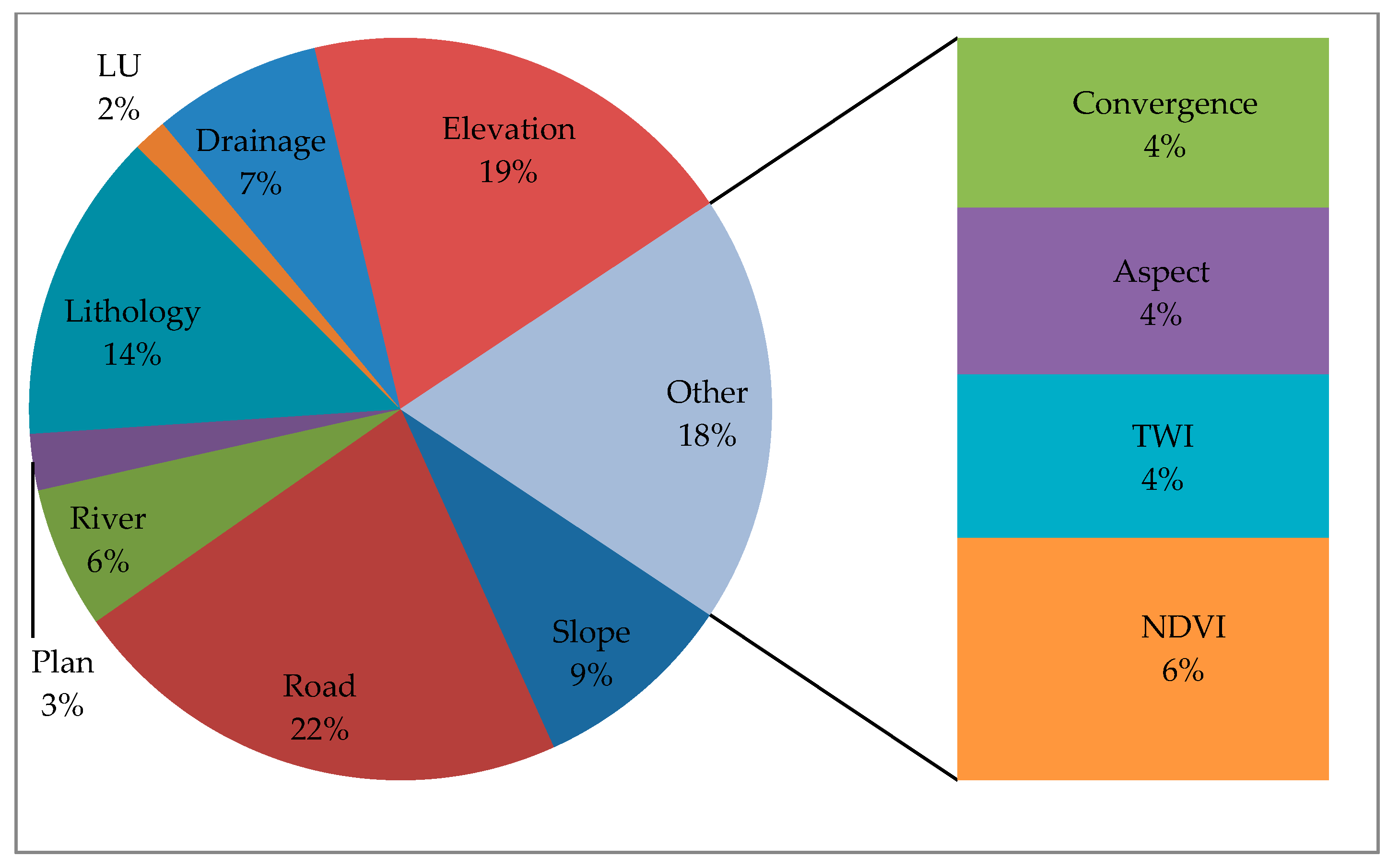
| Conditioning Factors | Weight |
|---|---|
| Distance from road | 381.67 |
| Elevation | 335.06 |
| Lithology | 234.21 |
| Slope degree | 153.85 |
| Drinage density | 126.72 |
| Distance from river | 106.84 |
| NDVI | 105.26 |
| Convergence index | 73.97 |
| Slope aspect | 72.41 |
| TWI | 71.3 |
| Plan curvature | 42.43 |
| LU | 25.38 |
| Models | AUC | Standard Error | Asymptotic Significant | Asymptotic 95% Confidence Interval | |
|---|---|---|---|---|---|
| Lower Bound | Upper Bound | ||||
| RF | 0.927 | 0.007 | 0.000 | 0.914 | 0.941 |
| MARS | 0.911 | 0.008 | 0.000 | 0.896 | 0.926 |
| BRT | 0.919 | 0.007 | 0.000 | 0.905 | 0.933 |
| Model | Susceptibility Classes | Total Area of Classes | Gully in Classes | No Gully Area (km) | Seed Cell (%) | SCAI | ||
|---|---|---|---|---|---|---|---|---|
| Area (km) | % | Area (km) | % | |||||
| RF | Very Low | 525.97 | 62.03 | 0.01 | 0.86 | 525.96 | 0.01 | 61.08 |
| Low | 148.28 | 17.49 | 0.04 | 5.67 | 148.24 | 0.24 | 0.74 | |
| Moderate | 79.42 | 9.37 | 0.11 | 14.80 | 79.31 | 1.15 | 0.08 | |
| High | 56.34 | 6.64 | 0.16 | 21.95 | 56.18 | 2.41 | 0.03 | |
| Very High | 37.88 | 4.47 | 0.41 | 56.72 | 37.46 | 9.27 | 0.00 | |
| MARS | Very Low | 339.01 | 39.98 | 0.02 | 2.10 | 339.00 | 0.04 | 10.45 |
| Low | 194.83 | 22.98 | 0.01 | 1.48 | 194.82 | 0.05 | 4.89 | |
| Moderate | 131.17 | 15.47 | 0.04 | 5.67 | 131.13 | 0.27 | 0.58 | |
| High | 77.35 | 9.12 | 0.08 | 11.59 | 77.26 | 0.93 | 0.10 | |
| Very High | 105.50 | 12.44 | 0.58 | 79.16 | 104.92 | 4.64 | 0.03 | |
| BRT | Very Low | 605.37 | 71.40 | 0.04 | 5.55 | 605.33 | 0.06 | 12.59 |
| Low | 88.38 | 10.42 | 0.03 | 4.56 | 88.34 | 0.32 | 0.33 | |
| Moderate | 52.01 | 6.13 | 0.06 | 8.26 | 51.95 | 0.98 | 0.06 | |
| High | 34.13 | 4.03 | 0.08 | 11.34 | 34.05 | 2.06 | 0.02 | |
| Very High | 67.98 | 8.02 | 0.51 | 70.28 | 67.46 | 6.40 | 0.01 | |
© 2018 by the authors. Licensee MDPI, Basel, Switzerland. This article is an open access article distributed under the terms and conditions of the Creative Commons Attribution (CC BY) license (http://creativecommons.org/licenses/by/4.0/).
Share and Cite
Arabameri, A.; Pradhan, B.; Pourghasemi, H.R.; Rezaei, K.; Kerle, N. Spatial Modelling of Gully Erosion Using GIS and R Programing: A Comparison among Three Data Mining Algorithms. Appl. Sci. 2018, 8, 1369. https://doi.org/10.3390/app8081369
Arabameri A, Pradhan B, Pourghasemi HR, Rezaei K, Kerle N. Spatial Modelling of Gully Erosion Using GIS and R Programing: A Comparison among Three Data Mining Algorithms. Applied Sciences. 2018; 8(8):1369. https://doi.org/10.3390/app8081369
Chicago/Turabian StyleArabameri, Alireza, Biswajeet Pradhan, Hamid Reza Pourghasemi, Khalil Rezaei, and Norman Kerle. 2018. "Spatial Modelling of Gully Erosion Using GIS and R Programing: A Comparison among Three Data Mining Algorithms" Applied Sciences 8, no. 8: 1369. https://doi.org/10.3390/app8081369
APA StyleArabameri, A., Pradhan, B., Pourghasemi, H. R., Rezaei, K., & Kerle, N. (2018). Spatial Modelling of Gully Erosion Using GIS and R Programing: A Comparison among Three Data Mining Algorithms. Applied Sciences, 8(8), 1369. https://doi.org/10.3390/app8081369