Gradient Correlation Functions in Digital Image Correlation

Abstract

The performance of seven different correlation functions applied in Digital Image Correlation has been investigated using simulated and experimentally acquired laser speckle patterns. The correlation functions were constructed as combinations of the pure intensity correlation function, the gradient correlation function and the Hessian correlation function, respectively. It was found that the correlation function that was constructed as the product of all three pure correlation functions performed best for the small speckle sizes and large correlation values, respectively. The difference between the different functions disappeared as the speckle size increased and the correlation value dropped. On average, the random error of the combined correlation function was half that of the traditional intensity correlation function within the optimum region.

1. Introduction

Digital image correlation (DIC), or Particle Image Velocimetry (PIV), has since its introduction in the 1980s evolved into one of the most versatile and widespread techniques in experimental mechanics [1,2,3,4,5,6]. Recent examples are found in diverse scientific fields such as biomechanics [7], infrastructure [8], material science [9], composite structures [10], and microfluidistics [11], but the technique is not restricted to these scientific fields. A quick search on a popular search engine lists over 50,000 contributions out of which 16,000 are published throughout the last four years. The great versatility of the technique comes from its simplicity and flexibility, scalability in both space and time, the fact that it is non-intrusive and that it produces deformation fields. Furthermore, the deformation fields can be generated as Lagrangian fields (typically used in DIC) or Eulerian fields (common in PIV), depending on which images that are compared. In general, the technique requires a unique feature to be present in the plane considered. In the absence of natural features, a pattern needs to be added, usually using spray (DIC) or by adding small particles to a flow (PIV). The general approach is then to follow the features in between successive frames using a model of the deformation field, which most often is performed locally involving a limited number of pixels, but global approaches have been demonstrated [6]. At the core of this calculation is a numerical optimization routine whose underlying function most often is defined as an intensity cross-covariance or as a sum of squared intensity differences. The performance of the two approaches differs only in details. It has been shown that the random error in the deformation calculation roughly scales with average feature size, subimage width and correlation value [12]. The quotient between subimage width and feature size defines in principle the number of independent contributions to the correlation and relates also to the reliability of the calculation. In addition, the feature size defines the curvature of the correlation peak and hence its susceptibility to random noise. The amount of random noise is specified by the correlation value. For a laser speckle pattern, the decay of the correlation value is almost completely dominated by speckle decorrelation, while for a white-light pattern algorithm dependent features such as precision in interpolation becomes important. This is the reason feature sizes slightly larger than the sampling limit often are preferred with these patterns.

Calculated image gradients are used frequently in DIC algorithms as a means of interpolation and as an aid to improve the performance of the optimization routine. Neggers et al. has recently published an extensive review of current algorithms using image gradients for DIC calculations [13]. The conclusions were that image gradients speed up search algorithms considerably and the most effective gradient vector is formulated from a weighted blend of image gradients from both images. However, these image gradients are used to speed up the search for the most probable set of correlation parameters. The underlying function is still an intensity correlation. On the other hand, feature detection based on image gradients are frequently used in computer-vision applications. For example O’Callaghan and Haga has published a paper on the use of a normalized gradient correlation function for detection of changes in a video stream [14]. The motivation for the use of gradient correlation in their application was mainly that the detection becomes more robust against varying background intensity. Such correlation functions have to my knowledge not yet been explored in connection with DIC.

The purpose of this paper is to investigate the performance of correlation functions based on derivatives of intensity images as a function of feature size and image degradation. Three fundamental normalized correlation functions are formulated based on intensity, intensity gradients, and intensity Hessian, respectively. From these an additional four correlation functions can be constructed as a combination of the three fundamental ones. These functions are then evaluated using simulations and experiments using laser speckles. The different correlation functions are introduced and discussed in Section 2. The set of evaluations are introduced and presented in Section 3 where the simulations are detailed in Section 3.1 and the experiments in Section 3.2, respectively. The paper ends with a discussion and some concluding remarks.

2. Theory

Consider two images $I_1\left({\mathbf{x}}_1\right)$ and $I_2\left({\mathbf{x}}_2\right)$ registered at the two time instances $t_1$ and $t_2$, respectively, containing approximately the same features. The images are assumed sampled on an $[M,N]$ sized grid with pixel pitch $[p_y,p_x]$ in row and column directions, respectively. It is assumed that the motions of the features between the two images are small wherefore local information can be used to estimate local motion. Apart from the intensities it is assumed that the gradient vector ${\mathbf{G}}_i\left({\mathbf{x}}_i\right)$ and the Hessian matrix $H_i\left({\mathbf{x}}_i\right)$ may be generated in each pixel, where $i=1,2$ for each of the images respectively. These additional fields are generated from application of the in-plane gradient column vector ${\nabla }_{\perp }={(\partial /\partial x,\partial /\partial y)}^t$ as ${\mathbf{G}}_i\left({\mathbf{x}}_i\right)={\nabla }_{\perp }I\left({\mathbf{x}}_i\right)$ and $H_i\left({\mathbf{x}}_i\right)={\nabla }_{\perp }I\left({\mathbf{x}}_i\right){\nabla }_{\perp }^t$, respectively. Associated with each pixel are therefore an intensity value, an intensity gradient vector, and an intensity Hessian matrix, respectively.

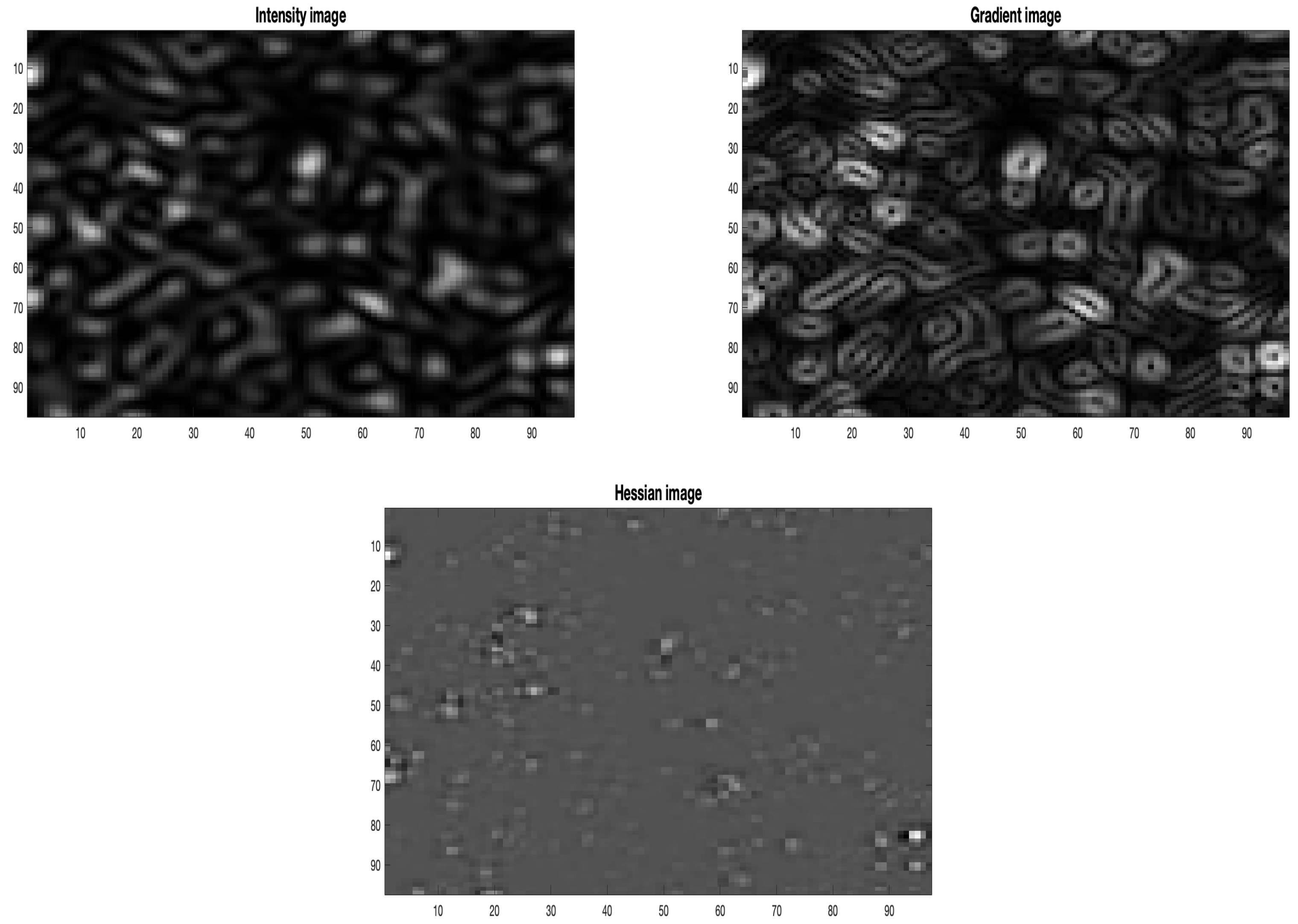
Figure 1 shows as a cropped example the intensity, the magnitude of the gradient vector and the determinant of the Hessian, respectively, of a laser speckle image. It is obvious that these three images contain different information and that they will perform differently in a correlation calculation. While the intensity image presents the distribution in intensity, the gradient image shows where the intensity changes most rapid. In regions with zero image gradient, the intensity correlation is essentially insensitive. The gradient image therefore dictates with what precision the intensity correlation function can be positioned. In addition, the Hessian matrix shows regions with a large intensity curvature. As the determinant can take on negative values, the background appears grayish, but regions close to speckle peaks light up. It is obvious that these peaks appear at the same positions as speckle maxima, but that they are locally more confined. Given these images, two continuous approximations of the intensity distributions can be formed using a nine-node quadratic Hermitian Finite Element. The intensity information in each node is taken from the intensity images and the gradient information required along the edges of the element is taken from the gradient and Hessian matrices, respectively. This approximation allows for a continuous description of image values, image gradients, and image curvatures, respectively, that is used throughout the remaining part of this paper.

An intensity correlation is usually expressed as,

$$CI(\Delta \mathbf{x})=\frac{\sum i_1({\mathbf{x}}_1+\Delta \mathbf{x})i_2\left({\mathbf{x}}_2\right)}{\sqrt{\sum i_1^2({\mathbf{x}}_1+\Delta \mathbf{x})\sum i_2^2\left({\mathbf{x}}_2\right)}},$$

(1)

where $i=I-<I>$ is the zero-mean intensity image, ${\mathbf{x}}_1$ and ${\mathbf{x}}_2$ are coordinates associated with the first and second image, respectively, and the summation is taken over all image points considered. The correlation variable, $\Delta \mathbf{x}$, contains all translations and translation gradients considered in the correlation. The general procedure in image correlation is to pick out a subimage of size $m\times n$ pixels from $I_1$ and search in $I_2$ for the set $\Delta {\mathbf{x}}_{max}$ of $\Delta \mathbf{x}$ that maximizes the correlation value $CI(\Delta \mathbf{x})$ in Equation (1). The two translation components $[u,v]$ of $\Delta {\mathbf{x}}_{max}$ are then taken as an estimate of the local displacement vector in the region of the chosen subimage. A displacement field is generated from repetition of the procedure for a multitude of different subimages. The random error, e, with which $[u,v]$ can be determined has been shown to vary as [12],

$$e=k\frac{S^2}{M}\sqrt{\frac{1-\gamma }{\gamma }},$$

(2)

where k is an algorithm dependent constant of order unity, S is the average feature size, $M=[m,n]$ is the correlation window width and $\gamma$ is the intensity correlation value. The quotient $M/S$ defines in principle the number of independent contributions to the correlation and relates also to the reliability of the calculation while the additional S defines the curvature of the correlation peak and hence its susceptibility to random noise. The amount of random noise is specified by the correlation value $\gamma$.

As with Equation (1), a gradient correlation may be expressed as,

$$CG(\Delta \mathbf{x})=\frac{\sum {\mathbf{G}}_1({\mathbf{x}}_1+\Delta \mathbf{x})·{\mathbf{G}}_2\left({\mathbf{x}}_2\right)}{\sqrt{\sum |{\mathbf{G}}_1({\mathbf{x}}_1+\Delta \mathbf{x}){|}^2\sum {|{\mathbf{G}}_2\left({\mathbf{x}}_2\right)|}^2}},$$

(3)

where $\mathbf{G}=\partial I/\partial x\widehat{\mathbf{x}}+\partial I/\partial y\widehat{\mathbf{y}}$ is the local image gradient vector, and $\widehat{\mathbf{x}}$ and $\widehat{\mathbf{y}}$ are orthogonal coordinate axes, respectively. Finally, a Hessian correlation function may be formulated as,

$$CH(\Delta \mathbf{x})=\frac{\sum \left[{\mathbf{v}}_{11}({\mathbf{x}}_1+\Delta \mathbf{x})·{\mathbf{v}}_{21}\left({\mathbf{x}}_2\right)+{\mathbf{v}}_{12}({\mathbf{x}}_1+\Delta \mathbf{x})·{\mathbf{v}}_{22}\left({\mathbf{x}}_2\right)\right]}{\sqrt{\sum \left[|{\mathbf{v}}_{11}{|}^2+{|{\mathbf{v}}_{12}|}^2\right]\sum \left[|{\mathbf{v}}_{21}{|}^2+{|{\mathbf{v}}_{22}|}^2\right]}},$$

(4)

where in the denominator special reference to ${\mathbf{x}}_1+\Delta \mathbf{x}$ and ${\mathbf{x}}_2$ are omitted for ease of reading. In Equation (4), ${\mathbf{v}}_{11}$ and ${\mathbf{v}}_{12}$ are the two orthogonal principal vectors associated with the local intensity Hessian of image $I_1$. The corresponding vectors for $I_2$ are expressed as ${\mathbf{v}}_{21}$ and ${\mathbf{v}}_{22}$, respectively.

The three correlation functions in Equations (1), (3) and (4) are all normalized between $[-1,1]$; however, their correlation features differ significantly. For example, as both the gradient correlation and the Hessian correlation involves vectors they are expected to drop off more quickly to a change in feature structure. Because of the normalization, the three correlation functions in Equations (1), (3) and (4) can be combined to produce the additional four correlation functions:

$$\begin{array}{cc}\hfill CIG(\Delta \mathbf{x})& =CI(\Delta \mathbf{x})CG(\Delta \mathbf{x}),\hfill \end{array}$$

(5)

$$\begin{array}{cc}\hfill CIH(\Delta \mathbf{x})& =CI(\Delta \mathbf{x})CH(\Delta \mathbf{x}),\hfill \end{array}$$

(6)

$$\begin{array}{cc}\hfill CGH(\Delta \mathbf{x})& =CG(\Delta \mathbf{x})CH(\Delta \mathbf{x}),\hfill \end{array}$$

(7)

$$\begin{array}{cc}\hfill CIGH(\Delta \mathbf{x})& =CI(\Delta \mathbf{x})CG(\Delta \mathbf{x})CH(\Delta \mathbf{x}).\hfill \end{array}$$

(8)

Hence, in total seven different correlation functions can be used to estimate the local deformation between the two set of images. Under what conditions either of them is preferable is investigated in the coming sections.

Figure 2 shows a comparison of the correlation properties between the seven correlation functions. The left image shows the width of the auto-correlation functions produced by setting $I_2=I_1$ in Equations (1) and (3)–(8), respectively, as a function of displacement $\Delta \mathbf{x}=u$. It is seen that all additional correlation functions are narrower and more well-defined than the intensity correlation. In particular all correlation functions that include the Hessian matrix have a significantly sharper peak. One may also notice that all mixed correlation functions are essentially free from ringing, which indicates that the background fluctuations generated from the three images are uncorrelated. The right image shows the drop-off in correlation as a response to an intensity decorrelation between the two images considered. These results were produced from simulated images with speckle diameter of five pixels and a $64\times 64$ pixels correlation window was used. Details are found in Section 3.1. It is seen in the right image of Figure 2 that the drop-off for the additional correlation functions are significantly quicker as compared to the intensity correlation. In particular, the functions that includes the Hessian correlation drops off fast. Whether this is a positive feature will be investigated in coming sections. In one respect, it is this feature that provides the sharp correlation peaks in the left image. However, a high sensitivity to small changes may also make the function unreliable.

3. Evaluation of Correlation Bases

The different correlation functions described in Section 2 are evaluated using simulations and are demonstrated on real images using laser speckles. In the simulations, the average speckle size is varied between three and seven pixels, and the speckle motion can vary randomly between $-5$ and 5 in both orthogonal directions, respectively. Simultaneously, the speckle correlation is varied between unity and 0.7. In all simulations the correlation window was chosen to be $32\times 32$ pixels and 225 independent windows are evaluated for each set of parameters. The reason for ignoring the effect of the correlation window size on the performance of the different correlation functions is that according to Equation (2) the important parameter to consider is the quotient $M/S$. Hence, it is sufficient to vary only the speckle size to capture the general behavior of the different correlation functions. The experiments were performed using laser speckles whose sizes were controlled by the objective aperture. In contrast to painted speckles, laser speckles are generated from random interference on the detector and do not exist on the object surface. Their extension thus depends on the numerical aperture of the imaging and on the wavelength of the laser [15]. In addition, for a well-focused system they will appear to follow the movement of the surface [16]. A set of ten rigid body translations were performed for each setting and the motion between the acquired images were analyzed in 225 independent regions with a correlation window size of $32\times 32$ pixels using each of the described correlation functions, respectively. Details are provided in the subsections below.

3.1. Simulations

The simulations are performed on computer generated laser speckle image pairs in accordance with the procedure described by Sjödahl and Benckert [17]. Consider an $N\times N$ matrix A filled with random complex numbers were the real and imaginary parts are independently picked from a normal distribution. In all simulations $N=1024$. The matrix A is taken to represent the exit pupil plane of a general imaging system. A quadratic aperture W of width $w=\lfloor N/S\rfloor$ pixels is placed centrally in the matrix, were S is the speckle size in pixels on the detector and $\lfloor ·\rfloor$ rounds down to the nearest integer. The reference speckle pattern $I_1$ is then generated as,

$$u_1(s_x,s_y)=W(s_x,s_y)A(s_x,s_y)⟶I_1(x,y)={|FT\left[u_1(s_x,s_y)\right]|}^2,$$

(9)

where $FT$ performs a 2D Fourier transform and $(s_x,s_y)$ are spatial frequency components spanning the domain $[-1/2,1/2-1/N]$ in both orthogonal directions, respectively. The deformed pattern $I_2$ is generated as,

$$u_2(s_x,s_y)=W(s_x,s_y)A(s_x-d,s_y)exp\left[2\pi i(u{s}_x+v{s}_y)\right]⟶I_2(x,y)={|FT\left[u_2(s_x,s_y)\right]|}^2,$$

(10)

where $d=\lfloor w(1-\sqrt{\gamma })\rfloor$ represents a shift of the exit pupil coherence cells between the two recordings, $\gamma$ is the intensity correlation value generated and $\mathbf{u}=[u,v]$ is the image plane speckle movement. In this way, speckle pattern pairs with a defined speckle size, S, relative motion, $\mathbf{u}$, and a defined intensity correlation, $\gamma$, can be generated. Mean deformation, standard deviation of the deformation magnitude, mean correlation value, and reliability are calculated for each of the speckle image pairs generated and for each of the seven correlation base functions. A single deformation estimate is in this case considered reliable if the estimate is within $\pm 1$ pixel from the correct value. The results from the simulations are shown in Figure 3.

3.2. Experiments

The experimental set-up is sketched in Figure 4. The set-up consists of a 10 mW continuous wave He-Ne laser (632.8 nm wavelength) as illumination source, a white-painted aluminum plate, an $f=55$ mm Mikro-Nikkor objective and a monochrome Dalsa nano camera (3.5 $\mathsf{\mu }$m pixel size, resolution $2056\times 2464$ pixels). The magnification was $m=0.9$ which translates into 3.9 $\mathsf{\mu }$m/pixel in object coordinates. One acquired speckle image with aperture setting $f/32$ is seen to the right in Figure 4. The experiments were performed with aperture settings $[f/22,f/16,f/11,f/8]$, which resulted in average speckle sizes $[7.6,5.5,3.8,2.7]$ pixels, respectively. Ten consecutive in-plane translations are performed using a fine-pitch micrometer. Each incremental translation was approximately 2.5 $\mathsf{\mu }$m, which translates into approximately 0.65 pixels on the detector. The total translation between the first and last image is therefore approximately 25 $\mathsf{\mu }$m, which translates into 6.5 pixels in detector coordinates. The result from the experiment is summarized in Figure 5. The reliability was unity for each of the analyzed image pairs, and is not presented separately.

4. Discussion and Conclusions

The structure highlighted in the three images in Figure 1 shows the different features that contributes to the different types of correlation functions defined by Equations (1), (3) and (4), respectively. These features are also responsible for the different shapes and drop-offs of the correlation functions shown in Figure 2. It is seen that out of the fundamental correlation functions, both the gradient correlation and to a greater extent the Hessian correlation produces a narrower and more well-defined peak and drops off more rapidly in response to feature degradations. With reference to the general behavior of correlation functions, these two effects should have contradictory effects on the accuracy of the deformation calculation [12]. The sharper peak should make the peak position more well-defined. The decrease in correlation value will on the other hand increase noise. The combined correlation functions show up a similar behavior with the most well-defined correlation peak produced by the multiplication of all three fundamental correlation functions. This is also the correlation function that drops off most rapid. One can also notice that this combined correlation function is basically free from higher order ringing, which indicates that the three fundamental correlation functions basically are uncorrelated.

A few interesting observations emerge from the results shown in Figure 3. For the high correlation values, the random errors always show up in the same order with the mixed correlation values the lowest. The difference between the best performing correlation function, which is the combination of all three fundamental functions, and the pure intensity correlation function is roughly a factor of two. The fundamental Hessian correlation performs constantly the worst, which is not surprising as the intensity Hessian is most susceptible to image noise. This disadvantage seems to be cancelled by multiplication with the other, more noise tolerant, correlation functions enhancing its advantage of being sharp. In fact, all mixed correlations involving the Hessian correlation performs well. One can also notice that the intensity correlation follows the general behavior $\sqrt{(1-\gamma )/\gamma }$, where $\gamma$ is the intensity correlation value for all speckle sizes, while the other correlation functions do not. In fact, for the smallest speckle sizes the mixed correlation functions involving the Hessian correlation seem to be more robust to decorrelation and show up an opposite curvature as compared with the pure intensity correlation. This effect seems to be valid up to a correlation of roughly 0.85 where these functions turns up and approach the other functions. At this point the combined correlation function is approximately three times more accurate as compared to the pure intensity correlation. This effect is not as pronounced for larger speckle sizes and for speckle sizes in the range 5–7 pixels all correlation functions perform approximately the same. By this one can notice two things. Firstly, for small speckle sizes both the gradient image and the Hessian image becomes more pronounced and will dominate in areas where they generate large numbers. Hence, their positive feature of being sharp is pronounced. As the features grow larger their relative weight decrease. An additional positive effect of this is for images that contain sharp edges. Such images are notoriously tricky to analyze using traditional intensity correlation, but with the combined correlations the gradient and Hessian correlations will act as filters, which actually is the motivation for the gradient correlation introduced by O’Callaghan and Haga [14]. Secondly, as the relative weight of the gradient and Hessian correlations decrease all three correlation functions behave approximately Gaussian and their combined effect will follow the same general trend. In addition, as they are uncorrelated their combined effect will also be Gaussian, and one gains very little to combine them. In conclusions therefore, combinations that include gradient and Hessian correlations contribute positively for sharp and dense patterns, but their positive effect decrease rapidly for larger features.

The reliability presented in the lower right corner of Figure 3 shows a dramatic behavior on speckle size and correlation value. It is seen that the reliability is always unity for highly correlated patterns for all speckle sizes and for all correlation functions. As the correlation drops the reliability starts to drop, in particular for the larger speckle sizes. As a matter of fact, the reliability drops to as low as 0.6 for a speckle size of 7 pixels and a correlation value of 0.7. The significant drop-off in reliability for the larger speckle sizes shown in Figure 3 is to a large extent associated with the pure Hessian correlation and to some extent the combined gradient and Hessian correlation. All other correlation functions are unaffected. The susceptibility of these two correlation functions comes from the magnification of noise caused by numerical differentiation in combination with a small sample size characterized by the quotient $N/S$, where in this case $N=32$ and S is the speckle size. A larger correlation window would significantly improve the reliability. As a matter of fact, it is recommended to keep the quotient $N/S$ above ten for reliable results in low-correlation images [12]. The reliability is therefore considered manageable for all relevant correlation functions considered.

The speckle image shown in Figure 4 shows a typical feature often encountered in practice, that of an uneven illumination. Uneven illumination is often difficult to circumvent as the intensity profile of most illumination sources is uneven. A TEM${}_{00}$ laser, for example, has a Gaussian beam profile. Unless compensated for, uneven illumination will bias the displacement estimate towards the brighter regions [12]. However not explicitly tested, one can speculate that the gradient and Hessian correlation functions would help to prevent this unwanted effect. In this investigation, however, no significant bias was noted.

The pattern shown in Figure 4 is a laser speckle pattern. A laser speckle pattern has the unique quality of providing a random pattern defined by the full spatial bandwidth of the field with unit contrast. Hence, the feature size of the pattern can be controlled by choosing an aperture size optimum for the resolution of the detector. The great disadvantage with laser speckles is that they decorrelate in response to any change in the optical set-up [16], an effect that has prevented widespread use of laser speckles in experimental mechanics. This effect is even more pronounced for the small numerical apertures used with former digital detectors. Modern lines of digital detectors can however be purchased with as small pixels as 1 $\mathsf{\mu }$m, which considerably opens up applications with laser speckles in experimental mechanics because of their ease of use. Figure 5 shows the results from application of the seven different correlation functions using the lens $f-$numbers $f/22$, $f/16$, $f/11$, and $f/8$, respectively. A dramatic dependence on lens $f-$number is seen for all correlation functions, in fact significantly more dramatic than any effect caused by the correlation functions themselves. For example, comparing the final deformation step for $f/22$ with the $f/8$ the random error is 0.73 with an intensity correlation value of 0.72 as compared with 0.02–0.04 and 0.90 for the larger aperture. This dramatic effect is caused by the double effect of enlarging the speckle size and enlarging the speckle decorrelation. In comparing the performance of the different algorithms for the same aperture settings the same trends as shown in Figure 3 are found. The random errors for the smaller speckle sizes and larger correlation values are about a factor of two smaller for the combined correlation functions as compared with the pure intensity correlation. The function combining all three pure correlations performs the best and the pure Hessian correlation the worst. The effect decreases for the larger speckle sizes and for lower correlation values. Finally, it was noted that the reliability turned out to be close to unity for all analyzed images with all correlation functions in contrast to the reliability of the simulated patterns. The reason for this discrepancy is however unknown.

In conclusion, the performance of seven different correlation functions applied in DIC have been investigated using simulated and experimentally acquired laser speckle patterns. The correlation functions were constructed as combinations of the pure intensity correlation function, the gradient correlation function and the Hessian correlation function, respectively. It was found that the correlation function that was constructed as the product of all three pure correlation functions performed best for the small speckle sizes and large correlation values, respectively, but that the difference between the different functions disappeared as the speckle size increase and the correlation value drops. On average the random error of the combined correlation function was half that of the traditional intensity correlation function within the optimum region. It was also found that for the small speckle sizes, all combined correlation functions involving the Hessian correlation function appear to be more robust against speckle decorrelation down to correlation values of roughly 0.85. The reason for this has not been investigated in detail but a good guess is that the more well-defined peak provided by the Hessian correlation makes its position more defined and less susceptible to noise. This effect disappears for smaller correlation values and for larger speckles. In addition, the monumental dependence of the imaging $f-$number on the accuracy of DIC using laser speckles is demonstrated experimentally. This dependence appears for all seven correlation functions and practically dominates the performance of the calculations. While the difference between the most optimum correlation function and the worst is in the order of three, the difference between results using different image apertures may be five times as large. Modern digital detectors with pixel sizes in the order of $\mathsf{\mu }$m may therefore open up for a renaissance of laser speckles in experimental mechanics, in particular in situations where a good random pattern is difficult to apply.

References

- Sutton, M.; Wolters, W.; Peters, W.; Ranson, W.; McNeill, S. Determination of displacements using an improved digital correlation method. Image Vis. Comput. 1983, 1, 133–139. [Google Scholar] [CrossRef]
- Bruck, H.; McNeill, S.; Sutton, M.; Peters, W. Digital image correlation using Newton-Raphson method of partial differential correction. Exp. Mech. 1989, 29, 261–267. [Google Scholar] [CrossRef]
- Willert, C.; Gharib, M. Digital particle image velocimetry. Exp. Fluids 1991, 10, 181–193. [Google Scholar] [CrossRef]
- Sjödahl, M. Electronic speckle photography: Increased accuracy by nonintegral pixel shifting. Appl. Opt. 1994, 33, 6667–6673. [Google Scholar] [CrossRef] [PubMed]
- Hild, F.; Roux, S. Digital image correlation: From displacement measurement to identification of elastic properties—A review. Strain 2006, 42, 69–80. [Google Scholar] [CrossRef]
- Hild, F.; Roux, S. Comparison of local and global approaches to digital image correlation. Exp. Mech. 2012, 52, 1503–1519. [Google Scholar] [CrossRef]
- Holenstein, C.; Lendi, C.; Wili, N.; Snedeker, J. Simulation and evaluation of 3D traction force microscopy. Comput. Methods Biomech. Biomed. Eng. 2019. [Google Scholar] [CrossRef] [PubMed]
- Alhaddad, M.; Dewhirst, M.; Soga, K.; Divriendt, M. A new photogrammetric system for high-precision monitoring of tunnel deformations. Proc. Inst. Civ.-Eng.-Transp. 2019, 172, 81–93. [Google Scholar] [CrossRef]
- Sjöberg, T.; Kajberg, J.; Oldenburg, M. Calibration and validation of three fracture criteria for alloy 718 subjected to high strain rates and elevated temperatures. Eur. J. Mech. A/Solids 2018, 71, 34–50. [Google Scholar] [CrossRef]
- Castillo, E.; Allen, T.; Henry, R.; Griffith, M.; Ingham, J. Digital image correlation (DIC) for measurement of strains and displacements in coarse, low volume-fraction FRP composites used in civil infrastructure. Compos. Struct. 2019, 212, 43–57. [Google Scholar] [CrossRef]
- Mouheb, N.; Montillet, A.; Solliec, C.; Havlica, J.; Legentilhomme, P.; Comiti, J.; Tihon, J. Flow characterization in T-shaped and cross-shaped micromixers. Microfluid. Nanofluid 2011, 10, 1185–1197. [Google Scholar] [CrossRef]
- Sjödahl, M. Accuracy in electronic speckle photography. Appl. Opt. 1997, 36, 2875–2885. [Google Scholar] [CrossRef] [PubMed]
- Neggers, J.; Blaysat, B.; Hoefnagels, J.; Geers, M. On image gradients in digital image correlation. Int. J. Numer. Meth. Eng. 2016, 105, 243–260. [Google Scholar] [CrossRef]
- O’Callaghan, R.; Haga, T. Robust Change-Detection by Normalised Gradient-Correlation. In Proceedings of the 2007 IEEE Conference on Computer Vision and Pattern Recognition, Minneapolis, MN, USA, 17–22 June 2007. [Google Scholar]
- Goodman, J.W. Statistical properties of laser speckle patterns. In Laser Speckle and Related Phenomena; Dainty, J.C., Ed.; Springer: Berlin, Germany, 1975; pp. 9–75. [Google Scholar]
- Yamaguchi, I. Speckle displacement and decorrelation in the diffraction and image fields for small object deformation. Opt. Acta 1981, 28, 1359–1376. [Google Scholar] [CrossRef]
- Sjödahl, M.; Benckert, L. Electronic speckle photography: Analysis of an algorithm giving the displacement with subpixel accuracy. Appl. Opt. 1993, 32, 2278–2284. [Google Scholar] [CrossRef] [PubMed]
Figure 1.
Images generated from the acquired set of intensity values. The upper left image shows the intensity distribution, the upper right image shows the magnitude of the calculated gradient vector, and the lower left image shows the determinant of the calculated Hessian matrix.
Figure 2.
Sensitivity of the different correlation functions. The left image shows the width of the different auto-correlation functions as a function of displacement. The right image shows the decrease in maximum correlation value as a function of intensity correlation value. These results are generated according to the theory in Section 2 and Section 3.1, respectively.
Figure 3.
Results from the simulation. The plots show, row-wise, random errors from the different types of correlation functions defined by Equations (1) and (3)–(8) as a function of intensity correlation value for speckle sizes 3, 4, 5, 6, and 7 pixels, respectively. The lower right plot shows the reliability of the evaluations as a function of intensity correlation.
Figure 4.
Sketch of the experimental set-up. The set-up consists of a 10 mW He-Ne laser, a monochrome camera from Dalsa equipped with a mikro-Nikkor camera objective with focal length mm, and a white aluminum plate that can be translated in-plane using a fine-pitch micrometer. The right part of the figure displays one of the acquired speckle images. This image is acquired with an aperture setting of .
Figure 5.
Random error in displacement as a function of speckle motion using different aperture numbers and analyzed using the seven different correlation functions. All results for the same aperture setting are lumped together.
© 2019 by the author. Licensee MDPI, Basel, Switzerland. This article is an open access article distributed under the terms and conditions of the Creative Commons Attribution (CC BY) license (http://creativecommons.org/licenses/by/4.0/).
Share and Cite
MDPI and ACS Style
Sjödahl, M. Gradient Correlation Functions in Digital Image Correlation. Appl. Sci. 2019, 9, 2127. https://doi.org/10.3390/app9102127
AMA Style
Sjödahl M. Gradient Correlation Functions in Digital Image Correlation. Applied Sciences. 2019; 9(10):2127. https://doi.org/10.3390/app9102127
Chicago/Turabian StyleSjödahl, Mikael. 2019. "Gradient Correlation Functions in Digital Image Correlation" Applied Sciences 9, no. 10: 2127. https://doi.org/10.3390/app9102127
Note that from the first issue of 2016, this journal uses article numbers instead of page numbers. See further details here.