Image Classification for Automated Image Cross-Correlation Applications in the Geosciences


Research Institute for Hydrogeological Protection, National Council of Research of Italy, 10135 Turin, Italy
*
Author to whom correspondence should be addressed.
Appl. Sci. 2019, 9(11), 2357; https://doi.org/10.3390/app9112357
Submission received: 1 April 2019
/
Revised: 9 May 2019
/
Accepted: 4 June 2019
/
Published: 8 June 2019
(This article belongs to the Special Issue Advances in Digital Image Correlation (DIC))
Abstract
:Featured Application
This study proposes a method that enables the automatic application of image cross-correlation when monitoring any displacements in the geosciences. As such, it solves one of the main current image processing issues: The requirement of manual image selection. The method reduces the need for extensive financial and human resources when conducting surveys, and it can be applied in a preventive warning context.
Abstract
In Earth Science, image cross-correlation (ICC) can be used to identify the evolution of active processes. However, this technology can be ineffective, because it is sometimes difficult to visualize certain phenomena, and surface roughness can cause shadows. In such instances, manual image selection is required to select images that are suitably illuminated, and in which visibility is adequate. This impedes the development of an autonomous system applied to ICC in monitoring applications. In this paper, the uncertainty introduced by the presence of shadows is quantitatively analysed, and a method suitable for ICC applications is proposed: The method automatically selects images, and is based on a supervised classification of images using the support vector machine. According to visual and illumination conditions, the images are divided into three classes: (i) No visibility, (ii) direct illumination and (iii) diffuse illumination. Images belonging to the diffuse illumination class are used in cross-correlation processing. Finally, an operative procedure is presented for applying the automated ICC processing chain in geoscience monitoring applications.
1. Introduction
Image cross-correlation (ICC) is a well-known methodology used in the geoscience field to measure earth surface dynamics and deformation phenomena [1,2,3,4]. Ground-based ICC applications enable observations of relatively fast natural processes at a medium range and at a high spatiotemporal resolution. In addition, the low costs, minimal equipment required to conduct photographic surveys and the certain degree of automation used in data processing, make ground-based ICC applications valuable tools for use in monitoring phenomena, even in harsh environments [3]. The adoption of an automated procedure for processing monitoring data allows high-frequency-updated results to be obtained without the need for continuous human supervision, and can be applied in early warning system applications, thereby reducing human and economic costs [5]. Different automatic approaches used to collect and process monitoring data have been reported in literature, such as those for the inclinometer [6], total station [7,8], ground-based SAR [9] and integrated systems [10].
However, the major limitation of the technology used in the ICC approach for natural phenomena monitoring, is its dependence on visual conditions, since adequate illumination (i.e., sunlight) and a complete view of the scene (i.e., clear sky) are required. This prevents an automated ICC procedure being applied in near-real-time that could be used for warning purposes, as a human intervention to selecting suitable images is required. In addition, the presence of shadows formed by the interaction between direct illumination and surface roughness can cause errors in the cross-correlation (CC) process, and this problem has often been considered in literature [1,11,12,13,14,15,16]. The most popular solution used to avoid such effects is to consider pictures that have a similar visual appearance, and have been acquired in a similar light (usually in the middle of the day [12,17,18] when the length of shadows is reduced, due to the higher sun elevation angle). However, Ahn and Box [12], and Giordan et al. [15] proposed the use of images acquired in conditions of diffuse illumination (such as the evening hours) when any shadows are minimal or absent. Both of these approaches involve the manual selection of images, and images with a partial or absent view (caused by fog or the presence of obstacles), and with non-homogeneous illumination, are thus discarded. In this respect, Gabrieli et al. [14] developed a method for automatically discarding images taken during adverse meteorological conditions; this involved analysing the mean and standard deviation of colour values along predefined lines in the image. Hadhri et al. [19] also automatically identified images containing artefacts, or where vision was obscured, using a posteriori statistical analysis based on image entropy. Furthermore, Schwalbe and Maas [16] developed a method for automatically detecting shadowed areas, and then removing them from the CC computation.
In our work, we describe a method of classifying images according to visible and illumination conditions that enables the selection of images with diffuse illumination. To correctly classify the images, we adopted a support vector machine (SVM) approach. This supervised machine learning method was originally developed by Boser et al. [20] and Cortes and Vapnik [21]; it is a well-known methodology used in remote sensing and geoscience, and it has been adopted in a wide range of fields and applications (please, see reviews in [22,23,24,25]). In addition, we present the use of completely automated processing in monitoring active gravitational processes through ICC. The principal innovation relies on applying autonomous image selection to ICC according to the a posteriori probability that an image belongs to a certain class of illumination.
2. Methods
The objective of this study was to develop a procedure that conducts image cross-correlation (ICC) autonomously, and which can be implemented for monitoring geophysical processes. The ICC method is briefly described in Section 2.1. As already mentioned, one of the main sources of uncertainty in ICC results relates to the presence of the shadows; therefore, the impact of shadows on the ICC is analysed here to demonstrate how they negatively affect any results (Section 2.2). With respect to this inherent problem, a method that autonomously selects images acquired with diffuse illumination is developed, and to achieve this, a support vector machine (SVM) is trained to distinguish between three classes of images in accordance with the presenting illumination (Section 2.3). Finally, an operative and autonomous procedure is designed to conduct ICC, with the aim of being used in geoscience monitoring applications (Section 2.4).
2.1. Image Cross-Correlation Processing
Digital image correlation (DIC) developed following the advent of performant computer machines and digital photography in the early 1990s, and has been applied predominantly in fluid dynamics [26,27] and satellite imagery [1]. The rationale behind DIC is to determine the field of motion using spatial cross-correlation between corresponding subsets of two images (image cross-correlation, ICC), where ICC analyses the texture of an image rather than specific recognisable elements (as in feature tracking methods [28,29]).
ICC can be computed in the spatial domain (direct cross-correlation, DCC) [1,3,26] or in the frequency domain (phase cross-correlation, PCC) using the discrete Fourier transform (DFT). In the former case, a subset of the original (master) image slides into a larger interrogation area of the slave image. In this respect, a two-dimensional (2D) correlation coefficient is computed for each possible position, and a map of correlation values is obtained. The coordinates of the element with the maximum correlation coefficient correspond to the displacement of the slave image in relation to the master. Although DCC requires high computational costs, it suffers less from decorrelation associated with motion, because it computes correlations between the same tiles in different positions (the Lagrangian approach). Conversely, the PCC computes the correlation between master and slave tiles (that are in the same position) into the image (the Eulerian approach). Therefore, part of the original texture is removed with respect to motion from the interrogation area, and this causes possible decorrelation. The PCC is computed through a complex product involving the Fourier transforms of the master and slave images, and this is equivalent to conducting a spatial cross-correlation in accordance to the convolution theorem.
In our work, the ICC is operated in the phase domain, as it provides a faster computation [30,31] process than DCC, but a similar performance [32]. Specifically, we use the two-step computation method proposed by Guizar-Sicairos et al. [33]. In the first run, the CC is computed with integer precision, thereby avoiding the zero-padding operation, and the centre of the slave matrix is then translated according to the shifts obtained. In the second run, the DFT is applied only to a small subset of the data to obtain subpixel accuracy. This method has the advantage of strongly limiting the zero-padding operation, thereby reducing the computational costs, and limiting the loss of information intrinsic in the PCC due to the Eulerian approach used in measurements [16,31].
The processing chain adopted in this study is based upon the approach presented in Dematteis et al. [34], and can be divided into four steps. First, certain image enhancement operations are conducted [12,13,14]. The scene illuminant is computed using principal components analysis (PCA) [35] and then subtracted from the trichromatic (RGB) image. The removal of the illuminant allows the reduction of possible low-frequency signals caused by illumination changes that can affect the computation of the DFT [36]. Subsequently, the image is converted to greyscale, and a sharpen mask is applied to enhance the details in the image texture. Such an operation aims to reduce any possible defocusing or blurring effects that are frequent in images acquired with limited illumination; in this respect, Ahn and Box [12] stated that the application of a sharpen mask can improve the ICC results in hazy situations. Second, the images are coregistered with respect to a common image to correct possible misalignments. The CC is computed on an area that is assumed to be stable, and the images are planarly translated according to the shifts obtained. Third, a sliding window identifies corresponding tiles on both the master and the slave images; the CC is then computed on the tile couples. Adjacent windows are overlapped by to improve the robustness of the results. Fourth, outlier removal is conducted. The usual approaches employed to correct possible outliers rely on heuristic and manual analysis [15,17], but Ahn and Box [12] identified outliers using cluster analysis during the CC procedure, and then applied a combined statistic-heuristic method in the post-interrogation phase. In this study, outlier correction is conducted using the universal outlier detection (UOD) approach [37] as this has the advantages of being automated, unsupervised, and non-subjective, which are fundamental requisites for automatic processing.
2.2. Analysis of Shadow Impact in ICC
Shadow lengths that change in relation to the sun’s position during the course of the day can affect the CC results by producing apparent motion. However, their influence has been rarely quantified [13,16]. For example, Travelletti et al. [13] observed that changes in illumination can lead to an average CC offset for images acquired over a time lag of 1–3 h, and also noticed that the correlation coefficient diminishes at a low sun elevation angle.
In this study, the effects of shadows on the results of the CC are investigated by considering four groups of images that have different illumination conditions: (i) Diffuse illumination; (ii) direct illumination in images acquired at the same hour in the day (12:00), when the sun azimuth and elevation were almost the same; (iii) direct illumination in images taken at different times during the day (i.e., when the sun was in different positions); and (iv) synthetic images produced from an existing digital surface model using a set of shaded reliefs. In the latter, the position of the lighting point was changed, thereby simulating the motion of the sun during the course of a day.
For each dataset, ICC was conducted for each possible pair of images and 45 CC maps were produced. The mean and standard deviation of the shifts for each map were then analysed, as these are associated with measurement accuracy and precision, respectively.
The possibility that a shadow’s presence could have differing effects on the CC results performed in phase or space domains was investigated, and the same analysis described above was conducted using both DCC and PCC. Results showed no relevant differences between the two techniques.
2.3. Image Classification
As previously mentioned, using images acquired in conditions that are diffusely illuminated enables a reduction in the apparent motion caused by changes in shadow shapes in relation to surface roughness. To this aim, it is fundamental that images are categorized in accordance with their visual appearance. In this study, three classes of visual and illumination states are considered: (i) Direct illumination (SunLight), (ii) diffuse illumination (DiffLight), and (iii) blocked or limited view (NoVis).
To identify the class of the images, SVMs are trained based on defining optimal decision hyper-planes that separate objects belonging to different classes [38]. In addition, the SVM assigns an a posteriori probability that each image belongs to a particular class. The objects are represented as vectors in an n-dimensional space, where the axes correspond to specific features that describe the objects. The elements of vectors represent feature values of each object that will be classified (for a didactic description of the SVM methods, please see Haykin [39]).
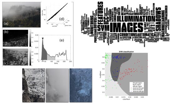
To describe the images, seven different features are identified as follows: (i) The number of RGB triplets (i.e., the values for R, G, and B bands) (colorNum), where the number of triplets is divided by the number of pixels in the image. The division is conducted to make the datum comparable for different image resolutions; (ii–iii) the number of pixels in the range 0–63 (blackNum) and 64–127 (greyNum) of the intensity histogram, which are determined using an 8-bit colour chart; (iv–v) the mean value of the hue (hueMean) and saturation (satMean) channels in the HSV colour space; (vi) the value of the maximum peak in the image intensity histogram (maxPeak), and (vii) the corresponding bin position (posPeak) (Figure 1). The image intensity (or greyscale) is defined as the mean value of the RGB channels.
We choose features that could be informative about the image appearance, and that were not correlated among them. Specifically, colorNum should be directly associated with the amount of light in the image, which enhances the colour contrast, while blackNum and greyNum indicate different levels of image darkness. hueMean is the average colour shade, and can be related to ambient skylight (i.e., diffuse illumination) [40], while satMean is high when the colours are vivid, and low when they tend toward grey. posPeak represents the dominant colour, while maxPeak is the magnitude of the dominant colour. Figure 1a shows an 8-bit (256 colour bins per RGB channel) NoVis class image. Only of the possible RGB triplets are present, which is evident from the narrow spatial distribution of the RGB values shown in Figure 1d. The upper portion of the picture has an almost uniform and grey colour that implies low satMean (Figure 1b); this produces a prominent dark peak (high maxPeak, low posPeak) (Figure 1e).
To reduce the dimensionality of the decision plane (i.e., to reduce the number of features used to train the SVM), a Monte Carlo cross-validation is conducted [41,42], with the aim of selecting a group of features (i.e., the estimator) that minimize misclassification errors. The fundamental of that approach is to randomly divide the available known data into two groups, one to train the SVM (training set) and one to evaluate the misclassification error (test set), and the feature selection procedure is repeated many times. Features are sequentially added to the candidate estimator by selecting the feature or group of features that minimize the misclassification error (averaged on the multiple iterates). This procedure guarantees a higher generality of the SVM and enables overfitting to be avoided.
To maintain generality no a priori information on the probability of class occurrence is introduced during the tuning of the SVM.
2.4. Automated ICC Procedure
The procedure presented here automatically selects images on which to perform ICC and obtains displacement maps of geophysical phenomena. This procedure was developed in 2018 and its effectiveness was tested in the monitoring of the Planpincieux glacier on the Italian side of the Mont Blanc massif. The processing chain is designed for automatic, continuous, and autonomous monitoring via ICC in the typical situation of daily acquisitions. The procedure is best suited for surveying natural phenomena at velocities greater than the common ICC uncertainty, i.e., ∼10−1 px [12,13]. It can thus be applied to observe relatively fast natural processes such as glacier flows and slope instabilities that are quite active. Depending on the phenomenon monitored, it is possible to vary the scheduled image acquisition and processing frequencies.
The procedure is conducted on a daily frequency and it is divided into four independent subroutines (Figure 2).
- (i)
- Image acquisition. First, the images are acquired at an hourly frequency by the monitoring system and are then transferred in real time to the data collection section of the operative server.
- (ii)
- Image classification and selection. The images acquired in the current day are classified through SVM according to the visual and illumination conditions. It is attributed a posteriori probability to belong to the classes. The results are saved in a list of classified images, and this list is subsequently browsed to search for the image with the highest probability score to belong to the DiffLight class. Such an image is labelled as suitable for ICC. If there are no new images, a warning is released and the process skips to the next subroutine.
- (iii)
- Image coregistration. This subroutine coregisters the new images acquired. A common reference image is used to coregister all the images and the coregistered images are saved. Such images are used for ICC and for possible manual vision inspection.
- (iv)
- Image cross-correlation. The list of images suitable for ICC is browsed to check for possible new image couples. If identified, the new images are cross-correlated and displacement maps are computed.
To evaluate the performance of the automated image selection, we manually classified the images and selected the images suitable for ICC. On several occasions (i.e., approximately of cases), manual classification of images was difficult, and there was a certain ambiguity between the classes. Therefore, three new bivalent classes were introduced relating to images that could be arbitrarily classified as either SunLight or DiffLight, SunLight or NoVis, and DiffLight or NoVis (respectively SD, SN, DN).
Moreover, the performances of automated selection through SVM were then compared with other possible simpler alternatives of automatic criteria. We analysed the cases of selecting images at a fixed hour of the day: At 12:00 (the SunLight class) and at 18:00 (the DiffLight class). To simulate such automated selection methods, photos were picked without applying quality control to verify whether the scene was adequately visible.
3. Dataset
To develop and test the analysis described in Section 2, various dedicated datasets were employed (Table 1). These comprise images of natural environment sites with heterogeneous geo-hydrological phenomena in north-western (NW) Italy (Figure 3). The generality of the method was thus strengthened by using a wide range of images.
Two different datasets comprise images from Monesi village (Liguria region, NW Italy), which is an Alpine village partially affected by a rotational slide activated during a flood in October 2016. MNS1 is the shaded relief extracted from a digital surface model (DSM) acquired using a drone and MNS2 is an RGB dataset acquired using a fixed camera installed on the opposite side of the valley.
The ACC dataset (Piemonte region, NW Italy) comprises a sequence of images acquired by a fixed camera installed to monitor the evolution of a large bedrock outcrop that has historically been affected by rock falls. During the monitoring period, there was no evidence of any slope instability activation in the area studied.
Three different datasets comprise images of the Mont de la Saxe rockslide (Valle d’Aosta region, NW of Italy); this is an active landslide with an estimated volume of that endangers the underlying village and road, which road provides access to the Mont Blanc tunnel, an important communication route between Italy and France [5,43,44,45]. The three different datasets that were acquired from three different view perspectives for this rockslide are SAXE2 and SAXE3, which were acquired by cameras positioned outside the area of gravitational instability, and SAXE1, the camera for which was installed on the rockslide and controlled one of the most active sectors.
SAXE3 is divided into two subsamples: SAXE3_a, which includes pseudo-random images taken in 2014 and 2015, and SAXE3_b, which is a time-lapse relating to the period 15–30 April 2014, when activity was pronounced, and a large failure occurred. There are no images included in either SAXE3_a or SAXE3_b.
The last dataset consists of images of the Planpincieux glacier on the Italian side of the Mont Blanc massif. The glacier is characterised by relevant kinematics and dynamics; numerous detachments from the snout have endangered the underlying hamlet of Planpincieux. This glacier has therefore been the subject of various remote sensing surveys in the recent past [15,34,46]. Two different cameras monitor the evolution of the glacier: PPCX1 acquires images of the lower part of the glacier while PPCX2 acquires images of the right lower tongue, the most active part of the glacier. The PPCX2 dataset, like the SAXE3 dataset, is divided into two distinct subsamples: PPCX2_a, which comprises images acquired during the years 2014–2017; and PPCX2_b, which includes the complete dataset acquired between 18 May and 3 October 2018. During this period, the automated ICC procedure described in Section 2.4 was applied in real time and more than 1500 images were collected.
The following text describes and discusses the use of every dataset in the procedures described in Section 2.2, Section 2.3 and Section 2.4.
To evaluate the effect of shadows we conducted two different analyses: (1) A synthetic set of ten shaded reliefs of a DSM was produced by changing the lighting source position to simulate the sun’s motion during the day. Shadows cast by obstacles were projected by computing the viewshed from the light source. Three of the ten shaded reliefs produced are shown in Figure 4a.1–a.3. (2) Ground-based RGB pictures of the same area acquired in different illumination conditions were considered. Three groups of ten images were selected that were acquired in (i) diffuse illumination (Figure 4(b.1)), (ii) direct illumination (Figure 4(b b.2)), and (iii) direct illumination at the same hour (at 12:00) (Figure 4(b b.3)), so that similar direct illumination was maintained in the photos.
An ensemble of seven datasets representing scenes from various natural environments was used to study the image classification methodology and to ensure that the method could be generalised. Specifically, datasets ACC, SAXE1, SAXE2, SAXE3_a, MNS2_b, PPCX1 and PPCX2_a were employed, and samples of images from these datasets acquired in different visual conditions are shown in
Figure 4c1–i3. Each dataset comprises photos belonging to different classes (i.e., acquired in different illumination and visual conditions), as catalogued during the process described in Section 2.3. The numbers of images in each class employed from the different datasets are presented in Table 2.
The images included in all the datasets were acquired during different years and seasons. The results showed that the SVMs classified the images accurately, even when dissimilar environmental conditions and morphological changes were presented. However, although it is considered that SVM training by adopting photos taken during specific seasons could improve its performance, this could result in a loss of generality.
The last application is automated ICC processing, and this was conducted using two-hourly time-lapses. The first dataset (PPCX2_b) comprised more than 1500 images, and it was collected to monitor the activity of the Planpincieux glacier from 18 May to 3 October. During this period, the automated ICC procedure described in Section 2.4 was applied in real time to monitor the glacier’s evolution. The second dataset used was SAXE3_b, where 139 images of the Mont de La Saxe landslides were selected. Table 3 shows the number of images employed from PCCX2_b and SAXE3_b datasets and their distribution among the different classes (considering also the bivalent classes described in Section 2.4).
4. Results
A quantitative analysis of how the shadow effects affect the ICC performance is presented in Section 4.1, and this demonstrates the negative impact of that phenomenon. In Section 4.2, the results of the Monte Carlo cross-validation are presented, with the aim of determining the best features that can be used to train the SVMs. Finally, Section 4.3 presents the results of the automatic ICC processing chain with respect to two operative case studies.
4.1. Shadow Impacts of ICC
The MNS2_a dataset comprises three groups of ten images with different illumination states. As the acquired scene is fixed, it is valid to assume that any possible change in the results relates principally to the shadow effect. Figure 5 shows a boxplot of the mean () and standard deviation () of the single CC maps of each group; these were computed for all possible image couples, and differentiated for the vertical () and horizontal () directions. It is evident that the dispersion of the two variables is at a minimum for the images acquired with diffuse illumination. Moreover, the obtained with images acquired at the same hour and in direct illumination are approximately two and three times greater, on average, than that obtained for images acquired in diffuse illumination. It is also evident that the of the horizontal component has slightly greater variability, while there are no significant differences between the two components for the .
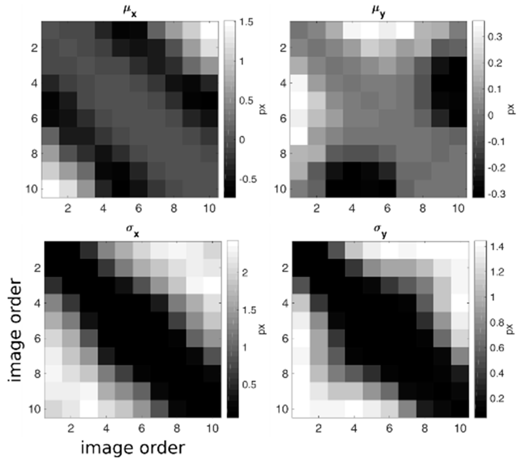
Figure 6 presents the and of the ICC maps produced using all of the couples of the available images from the dataset MNS1, where the results are ordered according to the simulated position of the sun during the day. The results obtained with synthetic shaded relief show that both and increase with an increase in the difference between the azimuth and elevation of the sun’s position. In addition, both values are higher for the horizontal direction, which indicates that the change in the sun’s azimuth has a greater effect on CC results than the change in elevation.
4.2. Cross-Validation and Image Classification
The results of the cross-validation (Table 4) show that the minimum classification curve is achieved by using three or four features to train the SVMs (Figure 7), where the minimum error obtained ranges between (with a weighted mean of ). In contrast, greater errors are obtained when more than four features are employed; this can probably be ascribed to overfitting in the training phase, as the number of training elements is limited.
The colorNum is evidently the predominant and most relevant feature in the classification. For each dataset, it is found to be the most important feature; it alone provides a misclassification error in the range of . hueMean is included in the group of relevant features in five of the datasets, whereas greyNum and satMean are never selected as relevant features. However, the features required for a proper training of the SVM differ between the datasets, and it is thus necessary to train a dedicated SVM for each specific scene.
For the MNS2_b dataset, a local minimum is achieved with only two features, while the absolute maximum is obtained with four features. Considering that this dataset comprises a limited number of images, training the SVM with two features is probably the best solution to avoid overfitting.
It is also worth noting that to select the minimum number of features, it may be a good criterion to use the features up to where the error curve decreases by less than when one more feature is added. Using this approach, two or three features would be sufficient, depending on the dataset.
Figure 8 shows an example of image classification using the two of the most relevant features obtained from the cross-validation (Table 4), to illustrate the migration of feature values among the different visual conditions. From the graph, it can be seen how colorNum increases from the NoVis, DiffLight and SunLight classes (which is expected) while hueMean of the SunLight class is lower.
4.3. Automated ICC Procedure
To evaluate the results of the automated ICC procedure, image classification and selection performances were analysed. Table 5 shows the results of automatic classification. In the case of images belonging to the bivalent class, an image was considered to be correctly classified if it was classified into one of the two classes that had been identified manually. Results therefore show that the classification error for dataset SAXE3_b is , while the selection error is . For dataset PPCX2_b, the misclassification is , while the error in determining whether the correct image should be included in the ICC processing is . For both datasets, the classification error is comparable with the value obtained during the cross-validation analysis. However, the selection error is related more to the occurrence of DiffLight false positives, which are higher in dataset PPCX2_b but considerably lower in SAXE3_b.
We also compared the ICC results obtained with automatic images selection through SVM, and the results of the automatic image selection using images selected at fixed hours, in conditions of direct and diffuse illumination. The correlation and mean absolute error (MAE) were computed with respect to results obtained using the manual selection of images (Table 6). The comparison was conducted pixel-by-pixel; therefore, more than and elements were considered for datasets SAXE3_b and PPCX2_b, respectively.
The results obtained with SVM selection show much higher correspondence with ICC results than the other two methods. Two principal factors provided lower performances in the other two selection methods: (1) As the state of view of the images was not controlled, it was possible to include images with obscured or partial views in the number of images that were processed; (2) the images with direct illumination suffered from the negative effects of shadows; therefore, any results for images with direct illumination are of a lower quality.
Furthermore, the correlation along the vertical direction was higher than that along the horizontal direction. As previously observed in the synthetic image analysis, the incidence of the sun’s azimuth angle is greater because its value varies more than the sun’s elevation, which influences the vertical direction. The MAEs of the vertical direction were thus greater because the values of displacement of these dimensions were greater.
Furthermore, a rather low correlation was noted between the horizontal direction of the images selected through SVM and those selected manually for the PPCX2_b dataset. An analysis of the absolute mean horizontal displacement value (Table 7) showed that this quantity was lower than the uncertainty. Therefore, the low correlation coefficient was likely due to the low signal-to-noise ratio.
5. Conclusions
This study quantitatively analyses the disturbing effect caused by the shape and length of shadows on the results of image cross-correlation (ICC). First, the impact of shadows on the development of an automatized procedure for the selection of images was determined, and it was demonstrated that adopting images acquired in conditions of diffuse illumination enables the shadow-related uncertainty to be minimized. Therefore, a possible solution was developed to ensure that the images selected were taken in diffuse illumination.
A method for automatically classifying the images according to the illumination appearance was then proposed. Considering photos taken of various natural environments (e.g., landslides, glaciers, rock faces), SVMs were trained using different features that were representative of the photo’s appearance. Of these, the number of RGB triplets was found to be the most significant feature used to discriminate between the classes. Training the SVMs with two or three features was sufficient for achieving an average misclassification error of .
The processing chain used to automatically select images suitable for ICC application, which includes the abovementioned classification method, is also described herein. The application of the method was applied during a survey campaign in 2018 to monitor the activity of the Planpincieux glacier for civil protection purposes, and the results showed that a high correspondence was obtained with results obtained using images selected manually. The same experiment was then conducted using time-lapse photos acquired for the Mont de La Saxe landslide.
These results show the possibility of developing a monitoring system based on ICC that automatically selects and processes the pictures acquired. The use of image sequence analysis enables financial and human resources to be reduced in monitoring active geo-hydrological instabilities. The development of an automatic solution is a valuable tool for use in developing an autonomous monitoring system that supplies daily updates.
Author Contributions
Conceptualization, N.D. and D.G.; methodology and analysis, N.D.; data curation, P.A.; writing—original draft preparation, N.D.; writing—review and editing, D.G.
Funding
This research received no external funding.
Conflicts of Interest
The authors declare no conflict of interest.
References
- Scambos, T.A.; Dutkiewicz, M.J.; Wilson, J.C.; Bindschadler, R.A. Application of image cross-correlation to the measurement of glacier velocity using satellite image data. Remote Sens. Environ. 1992, 42, 177–186. [Google Scholar] [CrossRef]
- Duffy, G.P.; Hughes-Clarke, J.E. Application of spatial cross correlation to detection of migration of submarine sand dunes. J. Geophys. Res. Earth Surf. 2005, 110, F04S12. [Google Scholar] [CrossRef]
- Delacourt, C.; Allemand, P.; Berthier, E.; Raucoules, D.; Casson, B.; Grandjean, P.; Pambrun, C.; Varel, E. Remote-sensing techniques for analysing landslide kinematics: A review. Bull. Société Géologique Fr. 2007, 178, 89–100. [Google Scholar] [CrossRef]
- Leprince, S.; Berthier, E.; Ayoub, F.; Delacourt, C.; Avouac, J.-P. Monitoring earth surface dynamics with optical imagery. EOS Trans. AGU 2008, 89, 1–2. [Google Scholar] [CrossRef]
- Wrzesniak, A.; Giordan, D. Development of an algorithm for automatic elaboration, representation and dissemination of landslide monitoring data. Geomat. Nat. Hazards Risk 2017, 8, 1898–1913. [Google Scholar] [CrossRef]
- Allasia, P.; Lollino, G.; Godone, D.; Giordan, D. Deep displacements measured with a robotized inclinometer system. In Proceedings of the 10th International Symposium on Field Measurements in Geomechanics—FMGM2018, Rio de Janeiro, Brazil, 16–20 July 2018. [Google Scholar]
- Manconi, A.; Giordan, D. Landslide early warning based on failure forecast models: The example of the Mt. de La Saxe rockslide, northern Italy. Nat. Hazards Earth Syst. Sci. 2015, 15, 1639–1644. [Google Scholar] [CrossRef]
- Allasia, P.; Baldo, M.; Giordan, D.; Godone, D.; Wrzesniak, A.; Lollino, G. Near real time monitoring systems and periodic surveys using a multi sensors UAV: The case of Ponzano landslide. In Proceedings of the IAEG/AEG Annual Meeting Proceedings, San Francisco, CA, USA, 17–21 September 2018; Springer: New York, NY, USA, 2019; Volume 1, pp. 303–310. [Google Scholar]
- Roedelsperger, S.; Becker, M.; Gerstenecker, C.; Laeufer, G. Near real-time monitoring of displacements with the ground based SAR IBIS-L. In Proceedings of the ESA Fringe Workshop, Frascati, Italy, 30 November–4 December 2009. [Google Scholar]
- Giordan, D.; Wrzesniak, A.; Allasia, P. The importance of a dedicated monitoring solution and communication strategy for an effective management of complex active landslides in urbanized areas. Sustainability 2019, 11, 946. [Google Scholar] [CrossRef]
- Berthier, E.; Vadon, H.; Baratoux, D.; Arnaud, Y.; Vincent, C.; Feigl, K.L.; Remy, F.; Legresy, B. Surface motion of mountain glaciers derived from satellite optical imagery. Remote Sens. Environ. 2005, 95, 14–28. [Google Scholar] [CrossRef]
- Ahn, Y.; Box, J.E. Glacier velocities from time-lapse photos: Technique development and first results from the Extreme Ice Survey (EIS) in Greenland. J. Glaciol. 2010, 56, 723–734. [Google Scholar] [CrossRef]
- Travelletti, J.; Delacourt, C.; Allemand, P.; Malet, J.-P.; Schmittbuhl, J.; Toussaint, R.; Bastard, M. Correlation of multi-temporal ground-based optical images for landslide monitoring: Application, potential and limitations. ISPRS J. Photogramm. Remote Sens. 2012, 70, 39–55. [Google Scholar] [CrossRef]
- Gabrieli, F.; Corain, L.; Vettore, L. A low-cost landslide displacement activity assessment from time-lapse photogrammetry and rainfall data: Application to the Tessina landslide site. Geomorphology 2016, 269, 56–74. [Google Scholar] [CrossRef]
- Giordan, D.; Allasia, P.; Dematteis, N.; Dell’Anese, F.; Vagliasindi, M.; Motta, E. A low-cost optical remote sensing application for glacier deformation monitoring in an alpine environment. Sensors 2016, 16, 1750. [Google Scholar] [CrossRef] [PubMed]
- Schwalbe, E.; Maas, H.-G. The determination of high-resolution spatio-temporal glacier motion fields from time-lapse sequences. Earth Surf. Dyn. 2017, 5, 861–879. [Google Scholar] [CrossRef] [Green Version]
- Debella-Gilo, M.; Kääb, A. Sub-pixel precision image matching for measuring surface displacements on mass movements using normalized cross-correlation. Remote Sens. Environ. 2011, 115, 130–142. [Google Scholar] [CrossRef] [Green Version]
- Messerli, A.; Grinsted, A. Image georectification and feature tracking toolbox: ImGRAFT. Geosci. Instrum. Methods Data Syst. 2015, 4, 23–34. [Google Scholar] [CrossRef] [Green Version]
- Hadhri, H.; Vernier, F.; Atto, A.M.; Trouvé, E. Time-lapse optical flow regularization for geophysical complex phenomena monitoring. ISPRS J. Photogramm. Remote Sens. 2019, 150, 135–156. [Google Scholar] [CrossRef]
- Boser, B.E.; Guyon, I.M.; Vapnik, V.N. A training algorithm for optimal margin classifiers. In Proceedings of the Fifth Annual Workshop on Computational Learning Theory, Pittsburgh, PA, USA, 27–29 July 1992; ACM: New York, NY, USA, 1992; pp. 144–152. [Google Scholar]
- Cortes, C.; Vapnik, V. Support-vector networks. Mach. Learn. 1995, 20, 273–297. [Google Scholar] [CrossRef]
- Pal, M.; Mather, P.M. Support vector machines for classification in remote sensing. Int. J. Remote Sens. 2005, 26, 1007–1011. [Google Scholar] [CrossRef]
- Mountrakis, G.; Im, J.; Ogole, C. Support vector machines in remote sensing: A review. ISPRS J. Photogramm. Remote Sens. 2011, 66, 247–259. [Google Scholar] [CrossRef]
- Lary, D.J.; Alavi, A.H.; Gandomi, A.H.; Walker, A.L. Machine learning in geosciences and remote sensing. Geosci. Front. 2016, 7, 3–10. [Google Scholar] [CrossRef] [Green Version]
- Maxwell, A.E.; Warner, T.A.; Fang, F. Implementation of machine-learning classification in remote sensing: An applied review. Int. J. Remote Sens. 2018, 39, 2784–2817. [Google Scholar] [CrossRef]
- Willert, C.E.; Gharib, M. Digital particle image velocimetry. Exp. Fluids 1991, 10, 181–193. [Google Scholar] [CrossRef]
- Westerweel, J. Fundamentals of digital particle image velocimetry. Meas. Sci. Technol. 1997, 8, 1379. [Google Scholar] [CrossRef]
- Lowe, D.G. Object recognition from local scale-invariant features. In Proceedings of the Seventh IEEE International Conference on Computer Vision, Kerkyra, Greece, 20–27 September 1999; Volume 2, pp. 1150–1157. [Google Scholar]
- Bay, H.; Ess, A.; Tuytelaars, T.; Van Gool, L. Speeded-up robust features (SURF). Comput. Vis. Image Underst. 2008, 110, 346–359. [Google Scholar] [CrossRef]
- Pust, O. Piv: Direct cross-correlation compared with fft-based cross-correlation. In Proceedings of the 10th International Symposium on Applications of Laser Techniques to Fluid Mechanics, Lisbon, Portugal, 10–13 July 2000; Volume 27, p. 114. [Google Scholar]
- Thielicke, W.; Stamhuis, E. PIVlab—Towards user-friendly, affordable and accurate digital particle image velocimetry in MATLAB. J. Open Res. Softw. 2014, 2, e30. [Google Scholar] [CrossRef]
- Bickel, V.; Manconi, A.; Amann, F. Quantitative assessment of digital image correlation methods to detect and monitor surface displacements of large slope instabilities. Remote Sens. 2018, 10, 865. [Google Scholar] [CrossRef]
- Guizar-Sicairos, M.; Thurman, S.T.; Fienup, J.R. Efficient subpixel image registration algorithms. Opt. Lett. 2008, 33, 156–158. [Google Scholar] [CrossRef] [PubMed] [Green Version]
- Dematteis, N.; Giordan, D.; Zucca, F.; Luzi, G.; Allasia, P. 4D surface kinematics monitoring through terrestrial radar interferometry and image cross-correlation coupling. ISPRS J. Photogramm. Remote Sens. 2018, 142, 38–50. [Google Scholar] [CrossRef]
- Cheng, D.; Prasad, D.K.; Brown, M.S. Illuminant estimation for color constancy: Why spatial-domain methods work and the role of the color distribution. JOSA A 2014, 31, 1049–1058. [Google Scholar] [CrossRef]
- Manduchi, R.; Mian, G.A. Accuracy analysis for correlation-based image registration algorithms. In Proceedings of the 1993 IEEE International Symposium on Circuits and Systems, Chicago, IL, USA, 3–6 May 1993; pp. 834–837. [Google Scholar]
- Westerweel, J.; Scarano, F. Universal outlier detection for PIV data. Exp. Fluids 2005, 39, 1096–1100. [Google Scholar] [CrossRef]
- Lary, D.J. Artificial intelligence in geoscience and remote sensing. In Geoscience and Remote Sensing New Achievements; Imperatore, P., Riccio, D., Eds.; InTech: Vienna, Austria, 2010; ISBN 978-953-7619-97-8. [Google Scholar]
- Haykin, S. Neural Network. A Comprehensive Foundation, 2nd ed.; Prentice Hall: Upper Saddle River, NJ, USA, 1999; ISBN 0-13-273350-1. [Google Scholar]
- Sunkavalli, K.; Romeiro, F.; Matusik, W.; Zickler, T.; Pfister, H. What do color changes reveal about an outdoor scene? In Proceedings of the 2008 IEEE Conference on Computer Vision and Pattern Recognition, Anchorage, AK, USA, 23–28 June 2008; pp. 1–8. [Google Scholar]
- Picard, R.R.; Cook, R.D. Cross-validation of regression models. J. Am. Stat. Assoc. 1984, 79, 575–583. [Google Scholar] [CrossRef]
- Xu, Q.-S.; Liang, Y.-Z. Monte Carlo cross validation. Chemom. Intell. Lab. Syst. 2001, 56, 1–11. [Google Scholar] [CrossRef]
- Crosta, G.B.; Di Prisco, C.; Frattini, P.; Frigerio, G.; Castellanza, R.; Agliardi, F. Chasing a complete understanding of the triggering mechanisms of a large rapidly evolving rockslide. Landslides 2014, 11, 747–764. [Google Scholar] [CrossRef]
- Crosta, G.B.; Lollino, G.; Paolo, F.; Giordan, D.; Andrea, T.; Carlo, R.; Davide, B. Rockslide monitoring through multi-temporal LiDAR DEM and TLS data analysis. In Engineering Geology for Society and Territory-Volume 2; Springer: New York, NY, USA, 2015; pp. 613–617. [Google Scholar]
- Manconi, A.; Giordan, D. Landslide failure forecast in near-real-time. Geomat. Nat. Hazards Risk 2016, 7, 639–648. [Google Scholar] [CrossRef]
- Dematteis, N.; Luzi, G.; Giordan, D.; Zucca, F.; Allasia, P. Monitoring Alpine glacier surface deformations with GB-SAR. Remote Sens. Lett. 2017, 8, 947–956. [Google Scholar] [CrossRef]
- Greene, C. Borders. In MATLAB Central File Exchange; MATLAB: Natick, MA, USA, 2019. [Google Scholar]
Figure 1.
(a) Original 8-bit trichromatic (RGB) image of NoVis class; (b) saturation map; (c) hue map; (d) 8-bit RGB values, and (e) intensity histogram in which the ordinate value of the black triangle indicates the maxPeaks and the abscissa value of the white triangle represents posPeaks features. The dark and light grey areas are blackNum and greyNum features, respectively.

Figure 2.
Workflow of an automated procedure used in image cross-correlation (ICC) applications.

Figure 3.
Locations of sites corresponding to the various datasets adopted. The black circle, square, and triangle correspond to Monesi di Mendatica, the Acceglio rock face, and the Mont de La Saxe landslide and Planpincieux glacier, respectively. This image was produced using the Matlab package borders [47].

Figure 4.
Examples of images taken from different datasets. Row (a) shows the 1st, 3rd and 7th shading reliefs with changes in the light source position; (b.2,b.3) were acquired in direct illumination at different hours of the day; and rows (c–i) show examples of each class from the datasets used in image classification analysis. The photographs in rows (j,k) were used to develop the automatic procedure.

Figure 5.
Boxplots of (a) mean and (b) standard deviation of CC. Subscripts D, 12 and S are as follows: D represents images acquired respectively with diffuse illumination, 12 denotes images with direct illumination taken at a fixed hour of the day (i.e., 12:00), and S concerns images taken in direct illumination with different sun azimuths and elevation angles.

Figure 6.
Mean and standard deviation of cross-correlation maps for all possible couples of shaded relief images. The two matrices on the left refer to the horizontal direction and those on the right refer to the vertical. The elements of the matrices correspond to the couples formed from the ith and jth images of a sequence of ten images that were ordered to simulate the motion of the sun during the day.

Figure 7.
Error curves (expressed as fraction of misclassification) obtained from cross-validation of the support vector machine (SVM) training. The minimum was always reached by employing three or four features.
Figure 7.
Error curves (expressed as fraction of misclassification) obtained from cross-validation of the support vector machine (SVM) training. The minimum was always reached by employing three or four features.

Figure 8.
Image classification of PPCX_1 images using the two principal features hueMean and colorNum. The regions delimit the areas where new elements within are classified as belonging to the corresponding class.
Figure 8.
Image classification of PPCX_1 images using the two principal features hueMean and colorNum. The regions delimit the areas where new elements within are classified as belonging to the corresponding class.


Table 1.
Datasets adopted in the current study. The first column lists the type of analysis employed using the various datasets. Also presented is the site where images were acquired for each dataset, the type of environment and image, the number of elements, the image resolution and the symbol attributed to the dataset.
| Analysis | Site | Environment | Image Type | # Images | Resolution [px] | Dataset Symbol |
|---|---|---|---|---|---|---|
| Shadow effect | Monesi | Alpine village | Shaded relief | 10 | 656 × 875 | MNS1 |
| Monesi | Rotational landslide | RGB | 30 | 3456 × 5184 | MNS2_a | |
| Image classification | Acceglio | Bedrock outcrop | RGB | 278 | 3456 × 5184 | ACC |
| La Saxe | Rockslide | RGB | 159 | 3240 × 4320 | SAXE1 | |
| La Saxe | Rockslide | RGB | 163 | 1536 × 2048 | SAXE2 | |
| La Saxe | Rockslide | RGB | 268 | 3312 × 4416 | SAXE3_a | |
| Monesi | Rotational landslide | RGB | 117 | 3456 × 5184 | MNS2_b | |
| Planpincieux | Glacier | RGB | 225 | 3456 × 5184 | PPCX1 | |
| Planpincieux | Glacier | RGB | 195 | 3456 × 5184 | PPCX2_a | |
| Automated ICC procedure | La Saxe | Rockslide | RGB | 139 | 3312 × 4416 | SAXE3_b |
| Planpincieux | Glacier | RGB | 1549 | 3456 × 5184 | PPCX2_b |
Table 2.
Numbers of images belonging to different classes used in each dataset.
| Dataset | SunLight | DiffLight | NoVis |
|---|---|---|---|
| A | 94 | 97 | 87 |
| B | 77 | 45 | 37 |
| C | 53 | 60 | 50 |
| D | 95 | 96 | 77 |
| E | 59 | 31 | 27 |
| F | 75 | 75 | 75 |
| G | 65 | 65 | 65 |
Table 3.
Number of images manually classified for datasets D1 and G1.
| Dataset | SunLight | DiffLight | NoVis | SD | SN | DN |
|---|---|---|---|---|---|---|
| D1 | 24 | 78 | 11 | 16 | 0 | 10 |
| G1 | 838 | 386 | 171 | 105 | 15 | 34 |
Table 4.
Order of features identified during cross-validation analysis for each dataset; features in black are those selected for classification.
Table 4.
Order of features identified during cross-validation analysis for each dataset; features in black are those selected for classification.
| Dataset | I | II | III | IV | V | VI | VII |
|---|---|---|---|---|---|---|---|
| ACC | colorNum | hueMean | maxPeak | posPeak | satMean | greyNum | blackNum |
| SAXE1 | colorNum | posPeak | hueMean | blackNum | maxPeak | greyNum | satMean |
| SAXE2 | colorNum | maxPeak | posPeak | hueMean | greyNum | satMean | blackNum |
| SAXE3_a | colorNum | hueMean | greyNum | maxPeak | satMean | posPeak | blackNum |
| MNS2_b | colorNum | blackNum | maxPeak | greyNum | hueMean | satMean | posPeak |
| PPCX1 | colorNum | hueMean | blackNum | posPeak | satMean | greyNum | maxPeak |
| PPCX2_a | colorNum | posPeak | hueMean | blackNum | maxPeak | greyNum | satMean |
Table 5.
Results of automatic classification and selection for datasets SAXE3_b and PPCX2_b. The number of images for each class are reported and correspond to exact, bivalent and erroneous classification. The percentage of correctly classified images is shown in the row below (in relation to the sum of exact and bivalent classifications). The two columns on the right show the percentage overall classification error and selection error, respectively.
| Dataset | SunLight | NoVis | DiffLight | Classification Error | Selection Error | ||||||
|---|---|---|---|---|---|---|---|---|---|---|---|
| SAXE3_b | |||||||||||
| 100% | |||||||||||
| PPCX2_b | |||||||||||
Table 6.
Correlation and MAE of two dimensions for dataset D1.
| Dataset | Method | ||||
|---|---|---|---|---|---|
| SAXE3_b | SVM | 0.69 | 0.18 | 0.84 | 0.24 |
| SunLight | 0.12 | 1.30 | 0.19 | 1.44 | |
| DiffLight | 0.38 | 0.44 | 0.69 | 0.57 | |
| PPCX2_b | SVM | 0.31 | 0.34 | 0.71 | 0.51 |
| SunLight | 0.02 | 1.78 | 0.14 | 2.21 | |
| DiffLight | 0.08 | 1.71 | 0.22 | 1.97 |
Table 7.
Mean absolute velocity and uncertainty of the two motion directions for two considered datasets; data are expressed in pixels.
Table 7.
Mean absolute velocity and uncertainty of the two motion directions for two considered datasets; data are expressed in pixels.
| Dataset | ||||
|---|---|---|---|---|
| SAXE3_b | ||||
| PPCX2_b |
© 2019 by the authors. Licensee MDPI, Basel, Switzerland. This article is an open access article distributed under the terms and conditions of the Creative Commons Attribution (CC BY) license (http://creativecommons.org/licenses/by/4.0/).
Share and Cite
MDPI and ACS Style
Dematteis, N.; Giordan, D.; Allasia, P. Image Classification for Automated Image Cross-Correlation Applications in the Geosciences. Appl. Sci. 2019, 9, 2357. https://doi.org/10.3390/app9112357
AMA Style
Dematteis N, Giordan D, Allasia P. Image Classification for Automated Image Cross-Correlation Applications in the Geosciences. Applied Sciences. 2019; 9(11):2357. https://doi.org/10.3390/app9112357
Chicago/Turabian StyleDematteis, Niccolò, Daniele Giordan, and Paolo Allasia. 2019. "Image Classification for Automated Image Cross-Correlation Applications in the Geosciences" Applied Sciences 9, no. 11: 2357. https://doi.org/10.3390/app9112357
Note that from the first issue of 2016, this journal uses article numbers instead of page numbers. See further details here.