Abstract
The present study proposes a method for model updating using measurements from sensors installed in arbitrary positions and directions. Modal identification provides mode shapes for physical quantities (acceleration strain, etc.) measured in specific directions at the location of the sensors. Besides, model updating involves the use of the mode shapes related to the nodal degrees-of-freedom of the finite element analytic model. Consequently, the mode shapes obtained by modal identification and the mode shapes of the model updating process do not coincide even for the same mode. Therefore, a method for constructing transform matrices that distinguish the cases where measurement is done by acceleration, velocity, and displacement sensors and the case where measurement is done by strain sensors was proposed to remedy such disagreement among the mode shapes. The so-constructed transform matrices were then applied when the mode shape residual was used as the objective function or for mode pairing in the model updating process. The feasibility of the proposed approach was verified by means of a numerical example in which the strain or acceleration of a simple beam was measured and a numerical example in which the strain of a bridge was measured. Using the proposed approach, it was possible to model the structure regardless of the position of the sensors and to select the location of the sensors independently from the model.
1. Introduction
In general, the model updating for a structure proceeds by minimizing the difference in the responses of the structure and of the model. The response of the structure can be physical quantities measured by sensors or be eigenvalues and mode shapes obtained by modal identification. Except for the eigenvalues, the measured quantities and the mode shapes are values specific to the location of the sensors. Considering that the location of the sensors does not generally coincide with the mesh of the finite element model, it is necessary to perform a proper transform that makes the location of the sensors match with the finite element model. Figure 1 shows a case where the location of the acceleration and strain sensors does not coincide with the position of the nodes in the model. In addition, the type of the measured physical quantities as well as the measurement direction shall be considered.
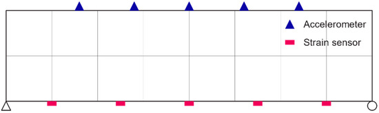
Figure 1.
Mismatch of measurement location and finite element mesh.
The modal identification extracting the dynamic characteristics of the structure from the measured data can be done in both the frequency domain and time domain. Frequency domain decomposition (FDD) [1] is a modal identification method in the frequency domain. The eigensystem realization algorithm (ERA) [2] and subspace identification method [3,4] are modal identification methods in the time domain. Such modal identification provides the natural frequencies of the structure at hand and the mode shapes for the measured physical quantities in the measurement direction at the location of the sensors.
The parameters of the numerical model can be derived by model updating using the so-obtained eigenvalues and mode shapes. The model updating methods can be divided into those relying on a deterministic approach [5,6] and those relying on a statistical approach [7,8,9,10]. The mode shapes obtained by eigen analysis in the model updating process are those related to the nodal degrees-of-freedom (DOFs) of the analytic model and differ from the measured mode shapes obtained by modal identification. Accordingly, it is necessary to provide a solution to remedy such a mismatch. Sanayei and Saletnik [11] introduced a transform matrix for the strain measurement to make the measured DOFs and model DOFs coincide and used the strain generated by static loading to perform model updating. Esfandiari, et al. [12] defined a frequency response function for the strain to perform model updating. However, these studies are limited to the case where the measurement direction of the strain sensors coincides with the longitudinal direction of the member and cannot be applied for sensors installed in arbitrary directions.
The survey shows that numerous studies were implemented on modal identification or model updating but stresses also the scarcity of studies on methods linking these two processes. Consequently, the present study intends to propose a systematic approach linking the modal identification results to model updating. Section 2 derives a method of achieving model updating using the data monitored by acceleration, velocity, displacement, and strain sensors installed in arbitrary locations and directions in the structure. Section 3 explains the proposed approach through a simple numerical example. In Section 4, the feasibility of the proposed approach is demonstrated through numerical examples for a bridge structure involving strain measurement with/without installation and measurement errors.
2. Materials and Methods
2.1. Measurement–Model Link
The eigenvector obtained by modal identification corresponds to that at the output measurement location. Besides, the eigenvector obtained by the analytic model is the one at the node DOF. In general, the output measurement location and the location of the node do not coincide, which means that these eigenvectors are at different locations. Moreover, the measurement direction is likely to differ from the DOF direction of the node. The type of eigenvector also differs between the measurement and the analytic model when the strain is measured. Accordingly, a solution is required to remedy the mismatch in the location, direction, and type between the measurement and the analysis. To that goal, the relation between the node DOFs of the analytic model and the measured values were derived.
The analytic model can be placed in any arbitrary position in the space, and various sensors such as accelerometers and strain gauges can be installed in each element of the analytic model (Figure 2). The spatial position in the analytic model is defined in the global coordinate system (GCS), and can be transformed into the element coordinate system (ECS). The location of the sensors and the measurement direction can be defined in the GCS or ECS. The measurement direction in the GCS is related to the measurement direction in the ECS as follows.
where the rotation matrix is as follows:
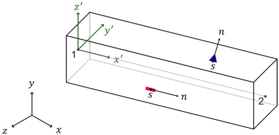
Figure 2.
Relationship between the global coordinate system and element coordinate system.
2.1.1. The Case Where the Displacement, Velocity, and Acceleration are Measured
The displacement measured in the measurement direction at the sensor location satisfies the following relationship with the displacement in the GCS at the sensor location.
where are the displacements in the directions of the GCS, respectively. The displacement in the GCS can be expressed in terms of the displacement in the ECS.
where are the displacements in the directions of the ECS.
The displacement in the ECS can be expressed as the product of the nodal displacement of the element and the shape function .
The DOFs and shape functions of an element vary according to the type of element used in the analytic model. The shape function for the two-dimensional Euler–Bernoulli beam element is arranged in Appendix A.
The displacement of the node of the element can be represented as follows by distinguishing the translational DOFs and the rotational DOFs. Some DOFs may vanish according to the element type.
where are the translational DOFs in the directions of the th node; and are the rotational DOFs with respect to axes of the th node. The corresponding displacement of the th node in the GCS can also be expressed similarly.
where are the translational DOFs in the directions of the th node; and are the rotational DOFs with respect to axes of the th node. The node displacement in the ECS satisfies the following relationship with the node displacement in the GCS.
The displacement in the measurement direction at the sensor location can be expressed by the node displacement in the GCS using Equations (4)–(12).
where
The so-derived relates to one sensor. Denoting for the th sensor by , matrix (where = the number of displacement sensors, = the number of DOFs of the analytic model) can be obtained for the whole set of displacement sensors by assembling the as follows.
Matrices ( = the number of velocity sensors) and ( = the number of acceleration sensors) can be obtained using the same method for the velocity and the acceleration, respectively.
The displacement , velocity , and acceleration in the measurement direction and at the sensor location can be expressed in terms of the node displacement , node velocity , and node acceleration in the GCS. Moreover, the displacement, velocity, and acceleration can also be expressed in terms of the eigenvector and the generalized coordinates for the displacement, velocity, and acceleration of the model, as shown in Equations (16)–(18). In addition, the mode shapes , , and for the displacement, velocity, and acceleration at the measurement location corresponding to eigenvector can be defined in terms of the transformation matrices , , and , as shown in Equations (19)–(21).
where
2.1.2. The Case Where the Strain is Measured
The method derived in Section 2.1.1 can be applied similarly for the strain. The strain measured at the sensor location can be expressed in terms of the strain in the ECS at the sensor location and the direction vector in the ECS.
where
The strain in the ECS can be rewritten in terms of the element node displacement using the displacement–strain transform matrix .
Matrix also varies according to the element type. The displacement–strain transform matrix for the two-dimensional Euler–Bernoulli beam element is arranged in Appendix A. Following the process formulated in Equations (7)–(12), the strain in the measurement direction and at the sensor location can be expressed in terms of the node displacement in the GCS.
where
The so-derived matrix relates to one strain gauge. Denoting for the th sensor by , matrix ( = the number of strain gauges) can be obtained for the whole set of sensors by assembling the as follows.
The strain in the measurement direction at the sensor location can be expressed by means of the node displacement in the GCS using this process. Moreover, the strain can be expressed by means of the eigenvector defined at the node DOF or the mode shape for the strain at the measurement location as shown in Equations (28) and (29).
where
The above process makes it possible to express the measured displacement, velocity, acceleration, and strain in terms of the node DOFs of the model. Moreover, the mode shapes , , , and for the measured values corresponding to the eigenvector of the node DOFs are also defined. The transform matrices and bridging the measurement and the analysis were derived solely using geometrical relations and are thus applicable, even in the case of change in the material’s characteristics. For convenience in the following, denotes the mode shape for the measured value and denotes the transform matrix to reduce Equations (19), (21), and (29) into the unique form expressed hereafter.
2.2. Model Updating
Model updating is the process by which the model parameters are updated using the measured data to make the numerical model behave as close as possible to the actual structure. The mode shape vector used during this process is the mode shape vector related to the node DOF. This is in contrast with the mode shape vector obtained by modal identification in relation to the physical quantities measured at the location and direction of the sensors. These two mode shape vectors thus have different forms. Accordingly, a method to make them fit with each other is necessary. Among them, model updating using the sensitivity method [5] is explained.
The basic formulation of model updating is as follows.
where ( = the number of compared variables) are the values obtained, respectively, by measurement and by analysis; and, ( = the number of model parameters) is the model parameter to be updated. This equation can be reformulated as follows for sensitivity analysis.
with
where is the number of iterations; is the residual; and, is the sensitivity matrix. The iteration proceeds by solving Equation (32) for to obtain of the next step until convergence.
The th eigenvalue and eigenvector of the analytic model are obtained from the stiffness matrix and the mass matrix .
2.2.1. Eigenvalue Residual
Being a behavioral characteristic of the entire structure, the eigenvalue is practically not affected by the location nor the type of sensor. However, the analytic mode shall be paired to its corresponding measured mode by the modal assurance criterion (MAC) [13] in order to compare the eigenvalue for the same mode. In such mode pairing, the analytic mode shape compared to the measured mode shape should be , obtained by Equation (30), and not .
Once the analytic mode corresponding to the measured mode is obtained, the residual and sensitivity matrices can be constructed as follows [14].
where are the mass and stiffness matrices of the analytic model; and, are the th eigenvalue and eigenvector. Here, the eigenvector shall be normalized for the mass matrix.
2.2.2. Mode Shape Residual
The mode pairing is performed by the method explained in Section 2.2.1 to make the comparison among corresponding modes. In addition, the measured mode shape and the analytic mode shape that have been paired may differ by a definite ratio and should thus be scaled by an appropriate method.
Mode scaling can be done for the measurement mode shape as well as for the analysis mode shape. Here, the measurement mode shape is scaled with respect to the analysis mode shape. The scaled measurement mode shape can be obtained as follows using the modal scale factor (MSF) [13] of the analytic mode shape for the measured mode shape .
where
where superscript * denotes the complex conjugate.
Once the scaled measurement mode shape is obtained, the residual and sensitivity matrices can be constructed as follows.
where the derivative with respect to the eigenvector can be obtained by previous studies [14,15]. The method of Fox and Kapoor [14] necessitates the whole eigenvectors to obtain the derivative for the th eigenvector, whereas the method of Nelson [15] provides a higher calculation efficiency since it uses only the th eigenvector to obtain the derivative.
3. Numerical Example
The simple numerical example shown in Figure 3 was adopted to explain numerically the method described in Section 2. The structure was a simply supported beam of 15 m with a height of 1 m and width of 0.5 m. The beam was modeled by two-dimensional Euler–Bernoulli beam elements. The elastic modulus was 25 GPa, the Poisson’s ratio was 0.2, and the density was 2300 kg/m3. The structural damping ratio for the 1st and 2nd modes was 5%. The strain gauges were installed at positions , , and . Assuming that the strain gauges were installed on the tendon for the introduction of the pre-stress force in a concrete structure, this layout allows not only the section strain but also the pre-stress force to be measured [16,17]. Accelerometers were installed vertically at the top of the center of each element.
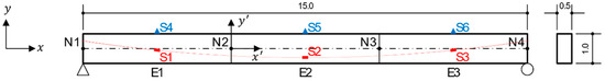
Figure 3.
Structure shape and sensor layout of numerical example (unit: m).
3.1. Modal Identification
Data measured by sensors were needed for modal identification but were generated analytically here. An initial velocity of −0.1 m/s was given vertically to nodes 2 and 3 in the model shown in Figure 3 to obtain the time histories of the displacement and acceleration at the sensor locations. These generated values were then adopted as measured data to perform modal identification, which provided the mode shape for the strain, the mode shape for the acceleration and the eigenvalue . For simplification, only the first mode was considered. For the first mode, and the mode shapes for the strain and the acceleration are as follows.
3.2. Construction of Transform Matrices
Since the GCS and ECS coincide, the rotation matrix was the identity matrix. The measurement direction of the strain gauges was , , and the measurement direction () in the ECS became , , and . The measurement direction of the accelerometers was and was in the ECS.
The strain components of the two-dimensional Euler–Bernoulli beam element were the longitudinal strain component () and the transverse strain component () induced by the Poisson effect. Matrix , which relates the strain () of the element and the displacement () of the node (subscripts 1 and 2 indicate, respectively, the first and second nodes of the element), can be obtained as follows using Equation (A3).
Transforming into , which relates the node and measurement directions in the GCS, gives
Assembling the transform matrices obtained for the strain gauges with respect to the global DOFs provides the transform matrix for the whole set of strain gauges.
where
In Equation (50), , , and , corresponding to the fixed DOFs, were 0 and could thus be discarded.
The displacement components of the two-dimensional Euler–Bernoulli beam element were the longitudinal component () and the transverse component (). Matrix , which relates the element displacement () and the node displacement, was obtained as follows using Equation (A6).
Transforming into , which relates the DOFs of the GCS and the displacement in the measurement direction, gives:
Assembling the transform matrices obtained for the accelerometers with respect to the global DOFs provided the transform matrix for the whole set of accelerometers.
where
3.3. Model Updating
As explained in Section 2.2, the model updating process was practically similar to previous model updating methods. The difference was that the mode shape of the node DOF of Equation (35) was not used as it was, but was transformed into the measured values as shown in Equations (40) and (41) when the residual for the mode shape was adopted as the objective function.
Model updating can be done for the measurement mode obtained from the strain sensors or for the measurement mode obtained from the acceleration sensors or for the mixed measurement mode from both types of sensors. Since model updating for the mixed measurement mode falls out of the scope of the present study, this case was not considered here.
Under the assumption that the initial elastic modulus of all the elements was 20 GPa, the model updating using the eigenvalue of the strain gauges, the measured mode , and the transform matrix gives an elastic modulus of 25 GPa for all the elements. This value corresponds to that of the model and demonstrates the feasibility of the proposed approach. Figure 4a shows the model updating process. The upper graph plots the change of the residual norm and the lower graph plots the changing norm for the difference between the final updated parameter and the parameter at each iteration. Only four iterations are needed to see that convergence was reached. In addition, the model updating using the eigenvalue of the accelerometers, the measured mode , and the transform matrix provided similar results. The convergence process in Figure 4b shows a similar pattern to the case where the strain was measured.
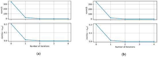
Figure 4.
Model updating process (a) when the strain was measured and (b) when the acceleration was measured.
The proposed approach was seen to allow model updating not only by means of the acceleration measurement but also by means of the strain measurement. There was also no need to limit the location of the sensors to the location of the nodes in the model. This means that the sensors can be installed at arbitrary locations inside the structure. Consequently, it was then possible to model the structure regardless of the position of the sensors and to select the location of the sensors independently from the model.
4. Numerical Application to Bridge
In order to verify the applicability of the proposed approach for large-scale structures, the numerical example shown in Figure 5 was established. The structure was a pre-stressed concrete box girder bridge with length of 50 m, height of 3 m, and width of 16.8 m. The bridge was composed of 19 segments and the material density was 2500 kg/m3. The damping ratio for the 1st and 2nd modes was 5%. A total of 50 strain sensors were installed longitudinally along the section bottom centerline at a spacing of 1 m, as shown in Figure 5b,c. This sensor layout can be achieved by only one quasi-distributed fiber optic sensor [18] based on resonance frequency mapping.
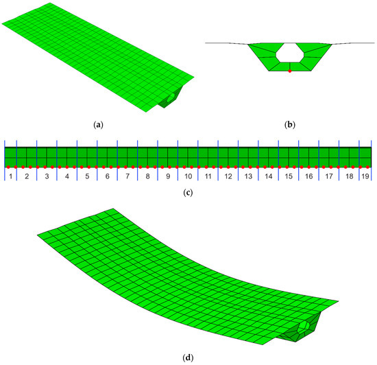
Figure 5.
Numerical application: (a) shape of the bridge structure, (b) layout of the strain sensors, (c) segments of the structure, and (d) first mode shape of the structure.
The structure was modeled using 556 four-node shell elements giving a total of 569 nodes and 3414 DOFs. Identical elastic moduli were assumed for the elements inside each segment. Except for segments No. 6 and No. 11, the elastic modulus of the segments was 30 GPa and was set to a value of 27 GPa for segments No. 6 and No. 11 with 10% damage. The eigenvalue analysis of the structure gave a natural frequency of 2.083 Hz for the 1st mode. The mode shape is shown in Figure 5d.
4.1. Without Uncertainties
An arbitrary load was applied vertically on the upper side of the structure and the strain was measured at a sampling rate of 100 Hz during 100 s. Figure 6a plots the strains measured by the 50 sensors. The application of the subspace identification method [4] to the measured strains provides the stabilization diagram shown in Figure 6b. The mode shape obtained when the system order was two is shown in Figure 6c. Here, the analytic solution was obtained directly from the mass and stiffness matrices of the structure. The mode shape obtained from the modal identification was seen to approach the analytic solution. The natural frequency for the mode at hand was 2.065 Hz and showed an error of merely 0.86% compared to the analytic solution (2.083 Hz).
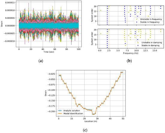
Figure 6.
Modal identification: (a) measured strains; (b) stabilization diagram; and (c) mode shape obtained by modal identification.
The elastic modulus of the model can be obtained by model updating using the eigenvalue and strain measurement mode shape provided by the modal identification. Figure 7a presents the iterative process shows fast convergence. Figure 7b compares the elastic moduli of the updated model with those of the structure and shows good agreement. Figure 7c plots the error ratio of the structure-updated model elastic moduli and reveals a maximum error of approximately 4%, which demonstrates that the model was fairly updated.
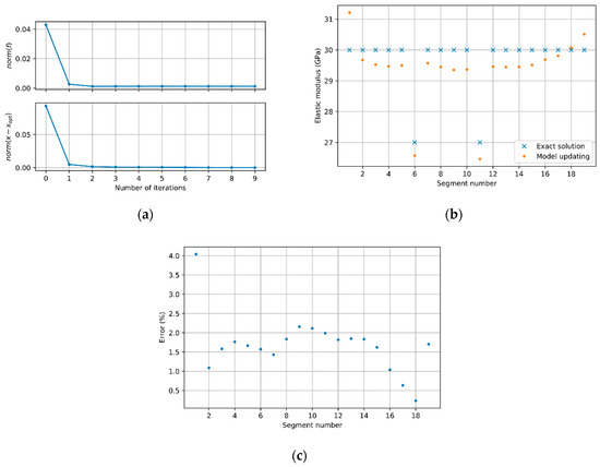
Figure 7.
Model updating results: (a) model updating process; (b) comparison of elastic moduli of the structure and updated model; and (c) error ratio of the structure-updated model elastic moduli.
In addition, the model updating using the eigenvalue and the strain measurement mode shape of the structure instead of the eigenvalue and the measurement mode shape obtained by modal identification resulted in elastic moduli identical to the exact solution of Figure 7a. This shows that the error observed in the model updating was generated during the modal identification process.
4.2. With Uncertainties
This section examines the effect of the various errors that may occur during the measurement of the model updating results. Errors in the installation of the sensor were considered to be caused by the uncertainties related to the position and the direction of the sensor. Error in the measurement was considered as white noise. Each error was assumed to have a normal distribution , with a zero mean and standard deviation . The standard deviation of the error in the installation of the sensor was set to 0 mm, 50 mm, and 100 mm for the position of the sensor and 0, 2, and 4 for the direction of the sensor considering the size of the error that may occur in a real situation. The standard deviation for the error with white noise was set to comparatively low levels of , , and under the assumption that the FBG sensor was installed. Model updating was performed 30 times for each considered case.
The following error was computed for each analyzed case and averaged for all identical cases to obtain the mean error ratio for each case.
where and are the elastic modulus and the updated elastic modulus of the ith segment of the bridge; and, is the number of segments (19 for the example). Figure 8 plots the mean error ratio for each case. The mean error ratio of the model updating was seen to increase with larger errors in the position of the sensor. On the other hand, the error relative to the direction of the sensor appears to have no significant effect on the mean error ratio of the model updating. Moreover, a larger measurement noise increased the mean error ratio but seemed to be uncorrelated to the error in the installation of the sensor.
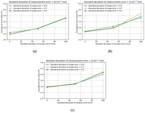
Figure 8.
Error ratio in model updating as a result of considering uncertainties in sensor position and direction and measurement noise: (a) without measurement error; (b) with standard deviation of in measurement error; (c) with standard deviation of in measurement error.
In Figure 8a, the case where the standard deviation for the position error was 0 mm and the standard deviation for the direction was 0 degree, it corresponded to the case without uncertainties in sub-Section 4.1. In such a case, the mean error ratio was 2.4%, which was the one produced during the modal identification process as explained above. The mean error ratio rose to 3.8% according to the increase of the error in the installation of the sensor. Note that, if the error introduced by the modal identification process was discarded, the mean error ratio caused by the installation error dropped to a minimal level of 1.4%. The mean error ratio, in the case with a standard deviation of for the measurement error in Figure 8c, ran between 3.0% and 4.2%. Here also, the error ratio caused only by the uncertainties in the installation and measurement remained very minimal with a level of approximately 0.6% to 1.8%. Consequently, the method proposed in this study is also applicable in cases including sensor installation errors and measurement noises.
5. Conclusions
A systematic approach using modal identification results in model updating was proposed. The mode shape obtained by modal identification and the mode shape of the model updating process did not coincide even for the same mode. A method constructing transform matrices considering cases where the measurement is done by acceleration, velocity, and displacement sensors and cases where measurement is achieved by strain sensors was proposed to remedy this disagreement among these mode shapes. The constructed transform matrices were applied when the mode shape residual was used as the objective function and for the mode pairing in the model updating process. The feasibility of the proposed approach was demonstrated through numerical examples involving strain or acceleration measurement with/without installation and measurement errors. The proposed approach allows the sensors to be disposed at locations representing appropriately the behavior of interest since the layout and direction of the sensors are not limited by the meshing of the model.
Author Contributions
Conceptualization, K.C. and J.-R.C.; Methodology, K.C.; Software, K.C.; Validation, K.C.; writing—original draft preparation, K.C.; Writing—review and editing, J.-R.C. and Y.-H.P.; Project administration, Y.-H.P.; Funding acquisition, Y.-H.P.
Acknowledgments
This research was funded by the Korea Institute of Civil Engineering and Building Technology, grant from a Strategic Research Project (Smart Monitoring System for Concrete Structures Using FRP Nerve Sensor).
Conflicts of Interest
The authors declare no conflict of interest.
Appendix A. Two-Dimensional Euler–Bernoulli Beam Element
As shown in Figure A1, the two-dimensional Euler–Bernoulli beam element has two nodes with the DOFs of Equation (A1).
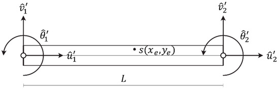
Figure A1.
DOFs of a two-dimensional beam element.
The strain at an arbitrary position in the element is formed by the longitudinal strain and the strain generated by the Poisson effect.
Matrix relating the node DOF of the element with the strain at an arbitrary position in the element is as follows.
where
The displacement at an arbitrary position in the element is formed by the longitudinal displacement and the transverse displacement .
Matrix relating the node DOF of the element and the displacement at an arbitrary position in the element is as follows.
References
- Brincker, R.; Zhang, L.; Andersen, P. In Modal identification from ambient responses using frequency domain decomposition. In Proceedings of the 18th International Modal Analysis Conference (IMAC), San Antonio, TX, USA, 7–10 February 2000. [Google Scholar]
- Juang, J.-N.; Pappa, R.S. An eigensystem realization algorithm for modal parameter identification and model reduction. J. Guid. Control Dyn. 1985, 8, 620–627. [Google Scholar] [CrossRef]
- Qin, S.J. An overview of subspace identification. Comput. Chem. Eng. 2006, 30, 1502–1513. [Google Scholar] [CrossRef]
- Van Overschee, P.; De Moor, B. Subspace identification for linear systems: Theory—Implementation—Applications; Springer Science & Business Media: Berlin, Germany, 2012. [Google Scholar]
- Mottershead, J.E.; Link, M.; Friswell, M.I. The sensitivity method in finite element model updating: A tutorial. Mech. Syst. Signal Process. 2011, 25, 2275–2296. [Google Scholar] [CrossRef]
- Mottershead, J.E.; Friswell, M.I. Model updating in structural dynamics: A survey. J. Sound Vib. 1993, 167, 347–375. [Google Scholar] [CrossRef]
- Yuen, K.V. Bayesian Methods for Structural Dynamics and Civil Engineering. John Wiley & Sons: Singapore, 2010. [Google Scholar]
- Katafygiotis, L.S.; Beck, J.L. Updating models and their uncertainties. Ii: Model identifiability. J. Eng. Mech. 1998, 124, 463–467. [Google Scholar] [CrossRef]
- Beck, J.L.; Katafygiotis, L.S. Updating models and their uncertainties. I: Bayesian statistical framework. J. Eng. Mech. 1998, 124, 455–461. [Google Scholar] [CrossRef]
- Mares, C.; Mottershead, J.; Friswell, M. Stochastic model updating: Part 1—Theory and simulated example. Mech. Syst. Signal Process. 2006, 20, 1674–1695. [Google Scholar] [CrossRef]
- Sanayei, M.; Saletnik, M.J. Parameter estimation of structures from static strain measurements. I: Formulation. J. Struct. Eng. 1996, 122, 555–562. [Google Scholar] [CrossRef]
- Esfandiari, A.; Sanayei, M.; Bakhtiari-Nejad, F.; Rahai, A. Finite element model updating using frequency response function of incomplete strain data. AIAA J. 2010, 48, 1420–1433. [Google Scholar] [CrossRef]
- Allemang, R.J. The modal assurance criterion–twenty years of use and abuse. Sound Vib. 2003, 37, 14–23. [Google Scholar]
- Fox, R.; Kapoor, M. Rates of change of eigenvalues and eigenvectors. AIAA J. 1968, 6, 2426–2429. [Google Scholar] [CrossRef]
- Nelson, R.B. Simplified calculation of eigenvector derivatives. AIAA J. 1976, 14, 1201–1205. [Google Scholar]
- Kim, S.T.; Park, Y.; Park, S.Y.; Cho, K.; Cho, J.R. A sensor-type pc strand with an embedded fbg sensor for monitoring prestress forces. Sensors 2015, 15, 1060–1070. [Google Scholar] [CrossRef] [PubMed]
- Cho, K.; Kim, S.; Cho, J.R.; Park, Y.H. Estimation of tendon force distribution in prestressed concrete girders using smart strand. Appl. Sci. 2017, 7, 1319. [Google Scholar] [CrossRef]
- Kim, G.H.; Park, S.M.; Park, C.H.; Jang, H.; Kim, C.S.; Lee, H.D. Real-time quasi-distributed fiber optic sensor based on resonance frequency mapping. Sci. Rep. 2019, 9, 3921. [Google Scholar] [CrossRef] [PubMed]
© 2019 by the authors. Licensee MDPI, Basel, Switzerland. This article is an open access article distributed under the terms and conditions of the Creative Commons Attribution (CC BY) license (http://creativecommons.org/licenses/by/4.0/).