Abstract
In carbon capture utilization and storage (CCUS) projects, the transportation of CO2 by ship can be an attractive alternative to transportation using a pipeline, particularly when the distance between the source and usage or storage location is large. However, a challenge associated with this approach is that the energy consumption of the liquefaction process can be significant, which makes the selection of an energy-efficient design an important factor in the minimization of operating costs. Since the liquefaction process operates at low temperature, its energy consumption varies with ambient temperature, which influences the trade-off point between different liquefaction process designs. A consistent set of data showing the relationship between energy consumption and cooling temperature is therefore useful in the CCUS system modelling. This study addresses this issue by modelling the performance of a variety of CO2 liquefaction processes across a range of ambient temperatures applying a methodical approach for the optimization of process operating parameters. The findings comprise a set of data for the minimum energy consumption cases. The main conclusions of this study are that an open-cycle CO2 process will offer lowest energy consumption below 20 °C cooling temperature and that over the cooling temperature range 15 to 50 °C, the minimum energy consumption for all liquefaction process rises by around 40%.
1. Introduction
Carbon capture utilization and storage (CCUS) refers to a wide-ranging set of techniques that can be used to mitigate anthropogenic CO2 emissions. Utilization methods include enhanced oil recovery (EOR), enhanced coal bed methane (ECBM), mineral carbonation, biological algae cultivation, conversion into synthesized fuels and chemicals feedstock. A recent review of the patents being published in field of CCUS concludes that, although the most patents concern utilization of CO2 in the production of fuels and chemicals, there are also a large number of patents published on algae cultivation, EOR, and ECBM [1].
The aim of many CCUS technologies is the re-use of CO2 emissions in the location where they are generated thereby eliminating any need for transportation and driving the development of a more circular economy. However, in the case of EOR and ECBM, a transportation step is usually needed, which can represent a significant challenge to the implementation of these types of CCUS projects [2,3]. Although there exists around 8000 km of CO2 pipeline in the world today, it is estimated that over 200,000 km of pipeline will be required by 2050 [4]. In addition, as the variety of CO2 sources considered in CCUS projects becomes more diverse, the challenges associated with transporting CO2 can be expected to multiply.
The transportation of CO2 by sea on a small scale has been a commercial practice in Europe for several years, where ships are used to transport food-quality CO2 from production plants to coastal distribution terminals [5]. The current commercial vessel sizes vary between 1000 and 1500 m3 and the transport pressure is in the range 14–20 bara [6]. Although the use of shipping in many CCUS projects would require a considerable scale-up in transport capacity, there are no technical barriers and shipping has long been identified as a potential option for the long-distance transport of CO2. The IPCC special report on CCS [5], for example, identifies shipping as the lowest cost option for distances over 1700 km. Other studies such as Mallon et al. [7] and Jakobsen et al. [8] have found that the trade-off distance for shipping could be much lower. As a result, shipping of CO2 is a standard feature in the modelling of CCS transportation networks and a significant number of studies have been made into the technical and commercial aspects of the liquefaction processes required, for example, the studies of Mitsubishi in 2004 [9], Jordal et al. in 2007 [10], and Roussanaly et al. in 2014 [11].
When transporting CO2 in ships, the energy consumption of the liquefaction process is significant, implying high operating costs. As a result, many studies have considered the design of the liquefaction process, particularly with a focus on reducing energy consumption. Hegerland [6] states that “in principle, there are two process alternatives” and goes on to suggest that when low temperature cooling water is available, CO2 should be used directly as a cooling medium, but above a trade-off temperature, an in-direct ammonia (NH3) refrigeration process becomes the best option. Subsequent studies have considered the selection of the optimal process flow scheme for the liquefaction of CO2 in more detail. Although the majority of work is focused on either open cycle CO2 processes or closed cycle NH3 refrigeration processes, others have also studied more novel approaches such as the use of absorption refrigeration [12], cascade refrigeration [13], and the application of turbo expanders [14]. Some have also compared a broad range of schemes. Alabdulkarem et al. [13], for example, compares simple refrigeration schemes, cascade refrigeration schemes, and absorption refrigeration schemes using waste heat. Most studies, however, focus on the performance of one or two schemes and one set of operating conditions.
In addition to the selection of the process flow scheme, the chosen CO2 transport pressure represents an important operating parameter for the liquefaction process. Hegerland [6] states that “to reduce investment costs of storage and ship tanks, it is required to operate as close to the triple point of 5.17 bara and −56.6 °C as practically feasible.” Aspelund et al. [15] and Lee et al. [16] looked at 6.5 bara transportation pressure based on the design of current commercial CO2 transportation by ship and also follow the assumption that the larger vessels used for CCS would operate at lower pressures. Decarre et al. [17] compared liquefaction at 7 bara and 15 bara, finding that transportation at 15 bara offers both lowest cost and lowest energy consumption. Seo et al. over the course of two papers, [18] and [19], also studied the optimum liquefaction pressure conditions finding that the overall cost was lowest for 15 bara cases. More generally, both Seo et al. [19], Alabdulkarem et al. [13], and Jackson et al. [20] found the optimum liquefaction pressure for the transportation of CO2 by pipeline to be around 50 bara, which is well above the practical limits for ship-based transport.
In addition to Hegerland et al. [6], Lee et al. [21] also investigated the relationship between cooling temperature and liquefaction process performance. However, both of these studies only consider liquefaction at low pressure and Lee et al. limit their study to the performance of open cycle CO2 processes. The approach taken by this study is, therefore, novel in as much as it studies how minimum energy consumption for a variety of different CO2 liquefaction process, operating at up to 15 bara, varies with cooling temperature. The results of this study are used to identify the trade-off point in terms of minimum energy consumption for NH3 and CO2-based systems. The main aim of this study is to present a consistent set of data for the variation in the minimum energy consumption of CO2 liquefaction across a range of ambient temperatures that can be used in the modelling a CCUS transportation systems.
2. Materials and Methods
The study method is set out below in two parts: first, a general description of the study approach is made, which breaks the methods employed into five steps; second, a more detailed description is presented for each of the five steps.
2.1. General Description
To begin with, a survey of previous studies was made to help identify the full range of possible process flow schemes available for the liquefaction process. Based on a review of the studies mentioned in the introduction, three were selected as the basis for further work that covered all of the principle flow scheme alternatives: Alabdulkarem et al. [13], Seo et al. [18], and Øi et al. [14]. From these three studies, four “base” flow schemes were then selected.
In the first phase of the modelling work, each of the four “base” schemes were modelled using the parameters from the study to which they belong. This exercise provided both a verification of the modelling approach and the correct interpretation of the design intent of each scheme. The performance of each scheme was then compared using a new common set of “base” parameters to allow an unambiguous comparison of the performance of each process. Importantly, the operating parameters for each of the process schemes were optimized with the “base” parameters for minimum energy consumption. After this, an additional set of process flow schemes was developed based on the most promising features from the schemes already modelled and finally, the performance of all schemes was compared to identify the best performing schemes to be use in the final phase of modelling work.
In the final phase of work, the performance of the best performing schemes was investigated over a range of ambient temperature conditions. At each temperature condition the operating parameters of each scheme were optimized to provide an accurate reflection of how performance varies with ambient temperature.
The method described above is summarized below as a five-step process. More detail on each of the individual steps is then presented below under separate sub-headings.
- Selection of “base” flow schemes and parameters
- Validation of the modelling basis
- Optimization and comparison of the “base” schemes
- Development and selection of the study basis
- Performance variation with cooling temperature
2.2. Selection of “Base” Flow Schemes and Parameters
The “base” schemes selected for this study were: a CO2-NH3 closed-loop refrigerant cascade scheme as Case 1 from Alabdulkarem et al. [13]; an NH3 based refrigeration scheme as Case 2 from Seo et al. [18] and as Case 3 from Øi et al. [14]; and an open-cycle CO2 scheme as Case 4, also from Øi et al. [14]. A process flow diagram for each of these schemes is presented in Figure 1.
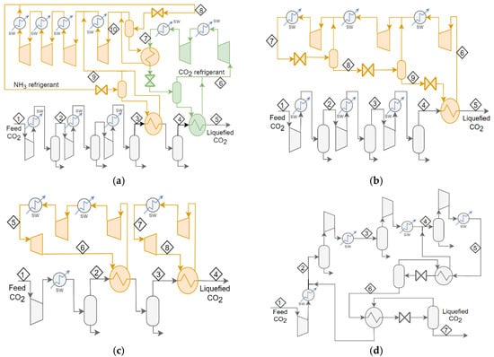
Figure 1.
Process flow diagrams for the “base” cases for the CO2 liquefaction schemes; (a) shows Case 1, (b) Case 2, (c) Case 3, and (d) Case 4.
Although each of these schemes was developed by the original study authors to achieve low energy consumption, each was developed based on a different set of modelling assumptions. A summary of the parameters used in each case is made below in Table 1.

Table 1.
Summary of modelling parameters.
To select a process scheme as the basis for this work, it was determined that the performance of each of the four “base” case schemes (Cases 1 to 4) should be compared on a consistent basis. This basis was selected based on a review of the range of the original operating parameters used in Cases 1 to 4. A review of the earlier work carried out by Jackson et al. [22] was also used to ensure compatibility with other related study work. The resulting “base” parameters are also summarized in Table 1.
Omitted from Table 1 is a summary of the CO2 compositions used as the basis in each of the cases. This is partly for the sake of brevity and partly because the composition of the CO2 stream used is not a focus of this study. For validation purposes, the CO2 feed stream compositions used in Cases 1 to 4 corresponded to the original study basis; in all subsequent work a pure stream of CO2 was used as the basis.
2.3. Process Modelling and Validation
A process model for each of the schemes was developed using Aspen HYSYS [23]. Operating conditions and energy flows were calculated using the Peng Robinson equation of state. Earlier studies have confirmed that the Peng Robinson equation of state generally provides reasonable accuracy in predicting the relevant properties for pure CO2 apart from the region immediately around the critical point [24,25].
To validate the modelling approach the flow schemes shown in Figure 1 were recreated with the parameters used in their original development. Where modelling parameters could not be determined directly by reference to the published data, assumptions were made. In Case 1 the temperature out of the NH2/CO2 exchanger was unknown and was, therefore, selected in this work to provide minimum overall power. In the study data published for Case 2, the compressor stage pressure ratios are not reported and, therefore, in this work a constant pressure ratio (equal to 2.1) was assumed. In Case 3, the number of compressor stages used in the LP ammonia refrigeration is unclear and in this work two compression stages are used to limit maximum temperature to 150 °C.
The detailed modelling results for each of the four validation cases are presented in Appendix A and a summary of the reported and modelled energy consumption is presented below in Table 2, which shows good agreement between the reported and modelled values.
Table 2.
Summary of the reported and modelled power consumptions for the “base” flow schemes.
It is worth noting that in Case 1, the energy consumption associated with pumping the CO2 product up to 150 bara is included in the model validation work although this is not needed for liquefaction at low pressure.
2.4. Optimization and Comparison of the “Base” Schemes
To ensure a consistent basis for the comparison of the four “base” flow schemes, the fixed set of “base” parameters shown in Table 1 were used in each of the cases. To ensure that the comparison was a fair one, the variable operating parameters for each case were optimized to achieve the minimum energy consumption for each case.
2.4.1. Implications of the “Base” Parameters
Implementation of the “base” parameters shown in Table 1 in the “base” flow schemes for Cases 1 to 4 (illustrated in Figure 1) has an impact on the flow scheme design in some cases. In Case 1, a cooling temperature of 25 °C and a maximum temperature of 150 °C requires one fewer stages in each of the three compressors compared to the “base” flow scheme illustrated in Figure 1a. In Case 2, the CO2 feed compressor also required one fewer stages for the 8.9 bara case compared to the scheme shown in Figure 1, but the NH3 compressor remained unchanged compared to the original design. In Case 3, due to a lower CO2 feed pressure, an extra stage is needed in the CO2 feed compressor. The low-pressure NH3 refrigeration compressors associated with Case 3 also require an additional stage to meet the 150 °C limit, but the high-pressure compressor is unchanged. In Case 4, the CO2 feed compressor also needs an additional stage, but the scheme is otherwise unchanged. Each of these modifications was implemented in the models developed for the “base” case flow schemes when making the comparisons of process performance for each case in this part of the study.
2.4.2. Optimization
The approach to optimization used in this study was to conduct the optimization outside of HYSYS using a link to MATLAB [26]. This link allowed the two-way transfer of process parameters between MATLAB and HYSYS and the implementation of the optimization algorithms directly in MATLAB.
The optimization algorithms used in MATLAB were fminsearch and GA. fminsearch uses a simplex algorithm that is suitable for unconstrained, multi-variable, non-linear optimization problems. A benefit of this method is that it will usually quickly converge to a solution; a downside is that in some cases a local minimum may be obtained. A drawback specific to the application of this algorithm in this study is that an unconstrained search can also lead HYSYS to non-viable solutions (e.g., where temperature crossing is inevitable in heat exchangers), which pauses the HYSYS solver and requires a time-consuming re-set of the optimization process. The GA algorithm can solve smooth or non-smooth optimization problems with or without constraints. It is a stochastic, population-based, algorithm, which is generally slower than fminsearch to reach a solution, but more reliable in solving the global minimum.
The objective of the optimization work was to minimize the energy consumption, which can be expressed as the sum of all compressor and expander stage energy consumptions:
where is the compressor discharge pressure level that is optimized, is the compression stage energy flows (CO2 and NH3 compressor stages are not differentiated here), is the expander stage energy flows (only relevant where an expander forms part of the process scheme), and
is the number of variable pressure specifications, which varies from case-to-case, as described in more detail below.
In Case 1, the condensing pressure in the CO2 refrigeration loop is set by the NH3 refrigeration process and the evaporating pressure is set by the liquefaction process; the maximum pressure in the NH3 refrigeration loop is set by the condensing temperature; and the discharge pressure from the first NH3 compressor stage is set by the liquefaction process. This leaves the two remaining pressure levels in the NH3 refrigeration compressor and the inter-stage pressure for the CO2 feed compressor as variables that can be optimized, giving .
In Case 2, the pressure level used in the second and third stages of the NH3 compressor are optimization variables along with the inter-stage pressure of the CO2 feed compressor, also giving .
In Case 3, the inter-stage pressure of the low pressure NH3 compressor is an optimization variable along with the inter-stage pressure of the CO2 feed compressor, making .
In Case 4, the discharge pressure for each of the CO2 compression stages is an optimization variable apart from the stage that occurs at the liquefaction pressure level, making .
When using the GA routine, the compressor stage outlet temperature was set as a constraint in the optimization algorithm for all cases:
where is the temperature at each of the compressor discharge pressure levels that can be optimized. When fminsearch was used, was checked manually and constrained, when necessary, by applying an appropriate constraint to an individual stage pressure level. Table 3 presents the results of the optimization work for the “base” process schemes (Cases 1 to 4).
Table 3.
Summary of optimized power consumption for the base process schemes.
2.5. Development and Selection of the Study Basis
The performance comparisons made using the “base” parameters as shown in Table 1 allowed the best performing processes to be identified from Cases 1 to 4 using the methods described above. The comparisons also helped—in some cases—to identify the potential improvements in the flow schemes. In particular, the use of expanders in place of valves in Case 4 was identified as a potential improvement along with the possibility of an additional stage of cooling in Cases 2 and 4.
The application of these features in the flow schemes for Cases 1 to 4 leads to the development of five new cases. The new cases as called Case 4b, which is Case 4 with expanders replacing valves; Cases 5a and 5b, which are developed from Case 2 by adding an extra cooling stage (5a with valves and 4b with expanders); and Case 6, which is developed from Case 4 by adding an additional stage and valves or expanders. Figure 2 and Figure 3 present the flow scheme for Cases 5 and 6.
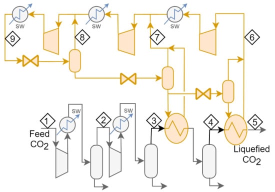
Figure 2.
Flow scheme for Case 5a. In Case 5b, each of the three letdown valves is replaced with an expander.
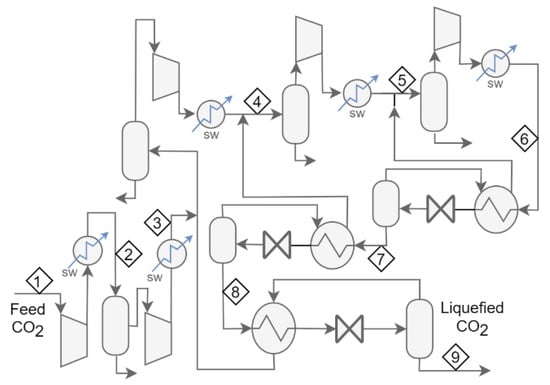
Figure 3.
Flow scheme for Case 6a. In Case 6b, each of the three letdown valves is replaced with an expander.
Each of these new cases were optimized following the same procedure as Cases 1 to 4. The number of optimization variables, , for Cases 5a and b are each less than Case 2 because the pressure level in the second stage of the NH3 compressor in Cases 5a and b is set by the temperature in the CO2 cooler (i.e., just above 0 °C). This gives for Cases 5a and 5b. Cases 6a and b have the same number of optimization variables as Case 4 (). Table 4 presents the results of the optimization work for Case 5 and Case 6.
Table 4.
Summary of optimized power consumption for the new process schemes.
Once the optimization process was complete, the best performing schemes were selected for the final part of the modelling work: the investigation of the impact of ambient temperature on energy consumption.
2.6. Performance Variation with Cooling Temperature
The method used to determine the Cases that would be studied in the final part of the modelling work was to first identify the best performing schemes and then second to consider what might represent the natural “next-best” process alternatives taking into consideration the complexity of each of the best performing cases. The selected cases were then optimized for temperatures in the range 15 to 50 °C aftercooler temperature.
3. Results
The main results of this study are presented below.
3.1. Process Modelling and Validation
The main results of the validation work, which are presented in the Method part of this paper, show that there is good agreement between the reference studies and the modelling work conducted here. As a supplement to this, the detailed modelling results for the validation cases are presented in Appendix A as Table A1, Table A2, Table A3 and Table A4. The stream numbering used corresponds to that shown in Figure 1.
3.2. Performance Comparisions
The energy consumption associated with each of the “base” process schemes (Cases 1 to 4) is presented below in Table 3. In all cases, the “base” operating parameters are used (see Table 1) and the values of all variable operating parameters are optimized to minimize energy consumption.
The results show that the 15 bara cases offer reduced power consumption in all of the “base” process schemes. They also show that a 3-stage NH3 process has the potential to outperform a 2-stage expander-based process and that a 2-stage open CO2 cycle can also offer low energy consumption. Based on these findings, Cases 4b, 5a, 5b, 6a, and 6b were developed. The performance of the optimized versions of these schemes is presented below in Table 4.
Table 4 shows that Case 6b offers lowest overall energy consumption when compared at 25 °C cooling temperature and that the use of expanders in the open CO2 refrigeration cycle offers a significant benefit over the use of valves. In the case of the NH3 refrigeration process, the benefit of using expanders is not as pronounced.
Based the results shown on Table 3 and Table 4, three cases were selected for study in the next part of the work: Case 6b, because it offers the lowest overall power; Case 6a because it offers a more conventional alternative to Case 6b; and Case 5a to provide a comparison with a NH3-based process. Case 5b was not selected because the addition of expanders offered little reduction in energy consumption compared to Case 5a. The detailed modelling results for the cases shown in Table 3 and Table 4 are presented in Appendix A.
3.3. Performance Variation with Cooling Temperature
Figure 4 shows how the energy consumption for Cases 5a, 6a, and 6b varies with ambient temperature. The smoothness of the three curves gives an indication of the level of consistency achieved in the optimization process. The results presented in Figure 4 illustrates the significant impact of cooling temperature on process performance and also, how at higher temperatures the performance of Case 5a improves relative to Cases 6a and 6b.
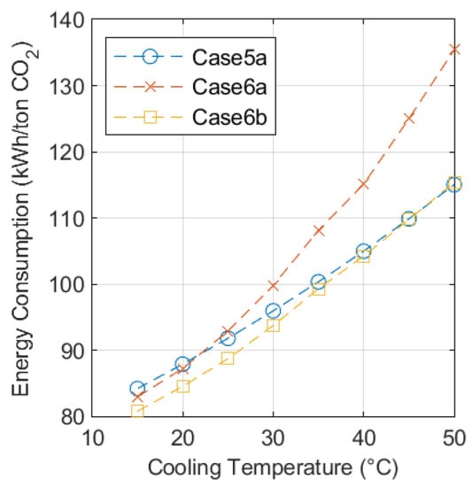
Figure 4.
Variation in energy consumption for Cases 5a, 6a, and 6b with cooling temperature.
Figure 5 shows the variation in the operating pressure parameters for Cases 5a, 6a, and 6b. Again, the smoothness of the two curves gives an indication of the level of consistency achieved in the optimization process. In both cases, the inter-stage pressure of the CO2 feed compressor drops as the cooling temperature increases. This is a result of the 150 °C temperature limits, which represents the optimum condition for inter-stage pressure in all the cases shown here.
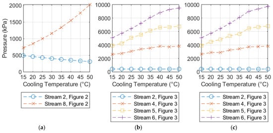
Figure 5.
Variation in the optimization parameters for Cases 5a (a), 6a (b), and 6b (c).
4. Discussion
Table 2 shows that the modelling approach used in this study is validated by comparing the results with other similar studies. Additionally, the smoothness of the curves presented in Figure 4 and Figure 5 shows that the optimization of the process parameters for Cases 5a, 6a, and 6b has been made on a consistent basis giving confidence in the trends illustrated in the results.
The variation of performance with ambient temperature presented in Figure 4 shows that Case 6a is the process that consumes the least energy across most of the temperature range studied. There is, however, a trade-off point around 45 °C, where Case 5a becomes the lowest energy consuming case. Case 6a does not offer the minimum energy consumption in any cases, but it does outperform Case 5a when the cooling temperature is below 20 °C. These trends support the original assertion of Hegerland [6] that open-cycle CO2-based systems outperform NH3-based refrigeration at low temperatures.
It is worth noting that the comparison between Case 5a and 6b is not entirely a fair one since the machinery required in Case 6b is significantly more complicated than that required in Case 5a. The potential benefit of a turbo expander-based process would ultimately be determined by the optimum balance between operating and capital costs, which in-turn will vary between projects. Also worth noting is that Case 4b offers similar performance to Case 6b with a small reduction in process complexity. Although the life-cycle costing of these schemes falls outside the scope of this study, the results provided here suggest that all of the Cases 4b, 5a, 6a, and 6b would merit consideration in a techno-economic study of the CO2 liquefaction process.
Cases 5a and 6a could be considered “conventional” and are also similar in the level of process complexity involved. Case 6a does, however, have a potentially significant advantage over Case 5a because of the possibility of condensing water out of the CO2 stream at pressure levels above the final liquefaction pressure. This will reduce, and possibly eliminate, the requirement for an additional dehydration step in the process. Therefore, in Case 5a an additional pressure-drop associated with a dehydration unit located prior to the liquefaction step may be necessary, representing a small additional energy penalty for this process. Again, the level of dehydration required and the energy penalty this represents would be expected to vary on a project-by-project basis.
5. Conclusions
As suggested by Hegerland [6] the energy consumption of open CO2-based refrigeration processes is found in this study to be lower than NH3-based refrigeration alternatives when ambient temperature is low. This study finds that the trade-off temperature also varies with the complexity of the specific processes considered: Case 6a has a trade-off point with Case 5a at a cooling temperature of 20 °C, whereas the more complex Case 6b has a trade off with 5a at 45 °C. The cooling temperature is also found to strongly influence the minimum energy consumption, which rises by around 40% for Cases 5a and 6b over the range 15 to 50 °C and by around 60% for Case 6a. This variation in energy consumption could be expected to be important for the accurate development of CCUS system models and the determination of the trade-off point between shipping and pipelines where the potential sources on disposal locations lie in locations with different ambient temperature conditions.
Author Contributions
Conceptualization, S.J.; Methodology, S.J. and E.B.; Validation, S.J.; Formal analysis, S.J.; Investigation, S.J.; Resources, S.J.; Data curation, S.J.; Writing—original draft preparation, S.J.; Writing—review and editing, S.J. and E.B.; Supervision, E.B.
Funding
This research received no external funding.
Conflicts of Interest
The authors declare no conflict of interest.
Appendix A
Appendix A1. Detailed Modelling Results for the Validation Cases
Table A1.
Mass balance for the Case 1 verification model, numbering as Figure 1a.
Table A1.
Mass balance for the Case 1 verification model, numbering as Figure 1a.
| Case 1 | 1 | 2 | 3 | 4 | 5 | 6 | 7 | 8 | 9 | 10 |
|---|---|---|---|---|---|---|---|---|---|---|
| Temperature (°C) | 38.0 | 38.0 | 38.0 | 1.00 | −45.1 | 38 | −48.1 | 38 | −2.7 | −16 |
| Pressure (bara) | 1.8 | 3.1 | 8.2 | 8.1 | 8.0 | 23.9 | 7.1 | 14.6 | 3.8 | 2.2 |
| Flow (ton/h) | 80.5 | 73.1 | 72.7 | 72.5 | 72.5 | 103.0 | 103 | 31.3 | 2.8 | 31.3 |
Table A2.
Mass balance for the Case 2 verification model, numbering as Figure 1b.
Table A2.
Mass balance for the Case 2 verification model, numbering as Figure 1b.
| Case 2 | 1 | 2 | 3 | 4 | 5 | 6 | 7 | 8 | 9 |
|---|---|---|---|---|---|---|---|---|---|
| Temperature (°C) | 35 | 35 | 35 | 35 | −28 | −36.7 | 35 | 7.80 | −15.2 |
| Pressure (bara) | 1.8 | 3.6 | 7.3 | 15 | 15 | 0.83 | 13.4 | 5.6 | 2.3 |
| Flow (ton/h) | 114 | 114 | 114 | 114 | 114 | 32.2 | 39.2 | 35.0 | 32.2 |
Table A3.
Mass balance for the Case 3 verification model, numbering as Figure 1c.
Table A3.
Mass balance for the Case 3 verification model, numbering as Figure 1c.
| Case 3 | 1 | 2 | 3 | 4 | 5 | 6 | 7 | 8 |
|---|---|---|---|---|---|---|---|---|
| Temperature (°C) | 20 | 15 | 1.0 | −50 | 15 | −55 | 15 | −4.0 |
| Pressure (bara) | 2.0 | 8.0 | 7.5 | 7.0 | 7.2 | 0.30 | 7.2 | 3.6 |
| Flow (ton/h) | 125 | 122 | 122 | 122 | 40.8 | 40.8 | 1.36 | 1.36 |
Table A4.
Mass balance for the Case 4 verification model, numbering as Figure 1d.
Table A4.
Mass balance for the Case 4 verification model, numbering as Figure 1d.
| Case 4 | 1 | 2 | 3 | 4 | 5 | 6 | 7 |
|---|---|---|---|---|---|---|---|
| Temperature (°C) | 20 | 10 | 15 | 14.4 | 15 | 3.7 | −48.5 |
| Pressure (bara) | 2.0 | 6.5 | 11.5 | 37.5 | 70.0 | 38.0 | 7.0 |
| Flow (ton/h) | 125 | 177 | 177 | 200 | 200 | 176 | 122 |
Appendix A2. Detailed Modelling Results for Optimised Base Cases
Table A5.
Mass balance Case 1, 15 bara liquefaction pressure, stream numbering from Figure 1.
Table A5.
Mass balance Case 1, 15 bara liquefaction pressure, stream numbering from Figure 1.
| Case 1 (15 Bara) | 1 | 2 | 3 | 4 | 5 | 6 | 7 | 8 | 9 | 10 |
|---|---|---|---|---|---|---|---|---|---|---|
| Temperature (°C) | 25.0 | 25.0 | 25.0 | 1.0 | −27.7 | −30.7 | 25.0 | 25.0 | −2.0 | −10.0 |
| Pressure (bara) | 1.00 | 4.01 | 15.6 | 15.3 | 15.0 | 13.6 | 28.7 | 9.95 | 3.94 | 2.87 |
| Flow (ton/h) | 100 | 100 | 100 | 100 | 100 | 130 | 130 | 33.0 | 1.96 | 33.0 |
Table A6.
Mass balance Case 2, 15 bara liquefaction pressure, stream numbering from Figure 1.
Table A6.
Mass balance Case 2, 15 bara liquefaction pressure, stream numbering from Figure 1.
| Case 1 (15 Bara) | 1 | 2 | 3 | 4 | 5 | 6 | 7 | 8 | 9 |
|---|---|---|---|---|---|---|---|---|---|
| Temperature (°C) | 25.0 | 25.0 | - | 25.0 | −27.7 | −32.7 | 25.0 | 13.0 | −1.48 |
| Pressure (bara) | 1.00 | 4.01 | - | 15.30 | 15.00 | 1.03 | 9.95 | 6.74 | 4.01 |
| Flow (ton/h) | 100 | 100 | - | 100 | 100 | 28.7 | 31.8 | 30.3 | 28.7 |
Table A7.
Mass balance Case 3, 15 bara liquefaction pressure, stream numbering from Figure 1.
Table A7.
Mass balance Case 3, 15 bara liquefaction pressure, stream numbering from Figure 1.
| Case 1 (15 Bara) | 1 | 2 | 3 | 4 | 5 | 6 | 7 | 8 |
|---|---|---|---|---|---|---|---|---|
| Temperature (°C) | 25.0 | 25.0 | 1.0 | −27.7 | 25.0 | −3.96 | 25.0 | −32.7 |
| Pressure (bara) | 1.00 | 15.6 | 15.3 | 15.0 | 9.95 | 3.65 | 9.95 | 1.03 |
| Flow (ton/h) | 100 | 100 | 100 | 100 | 1.96 | 1.96 | 29.2 | 29.2 |
Table A8.
Mass balance Case 4, 15 bara liquefaction pressure, stream numbering from Figure 1.
Table A8.
Mass balance Case 4, 15 bara liquefaction pressure, stream numbering from Figure 1.
| Case 1 (15 Bara) | 1 | 2 | 3 | 4 | 5 | 6 | 7 |
|---|---|---|---|---|---|---|---|
| Temperature (°C) | 25.0 | 19.3 | 25.0 | 23.6 | 25.0 | 9.44 | −27.7 |
| Pressure (bara) | 1.00 | 14.7 | 27.8 | 43.9 | 65.0 | 44.2 | 15.0 |
| Flow (ton/h) | 100 | 138 | 138 | 191 | 191 | 138 | 99.3 |
Appendix A3. Detailed Modelling Results for New Cases
Table A9.
Mass balance for Case 4b, stream numbering from Figure 1.
Table A9.
Mass balance for Case 4b, stream numbering from Figure 1.
| Case 4b | 1 | 2 | 3 | 4 | 5 | 6 | 7 |
|---|---|---|---|---|---|---|---|
| Temperature (°C) | 25.0 | 19.8 | 25.0 | 23.7 | 25.0 | 10.2 | −27.7 |
| Pressure (bara) | 1.00 | 14.7 | 28.0 | 44.7 | 65.0 | 45.0 | 15.0 |
| Flow (ton/h) | 100 | 135 | 135 | 182 | 182 | 134 | 100 |
Table A10.
Mass balance for Case 5a, stream numbering from Figure 2.
Table A10.
Mass balance for Case 5a, stream numbering from Figure 2.
| Case 5a | 1 | 2 | 3 | 4 | 5 | 6 | 7 | 8 | 9 |
|---|---|---|---|---|---|---|---|---|---|
| Temperature (°C) | 25.0 | 25.0 | 25.0 | 1.00 | −27.7 | −32.7 | 2.11 | 12.9 | 25.0 |
| Pressure (bara) | 1.00 | 4.01 | 15.6 | 15.3 | 15.0 | 1.03 | 3.94 | 6.73 | 9.95 |
| Flow (ton/h) | 100 | 100 | 100 | 100 | 100 | 26.8 | 3.39 | 1.51 | 31.7 |
Table A11.
Mass balance for Case 5b, stream numbering from Figure 2.
Table A11.
Mass balance for Case 5b, stream numbering from Figure 2.
| Case 5b | 1 | 2 | 3 | 4 | 5 | 6 | 7 | 8 | 9 |
|---|---|---|---|---|---|---|---|---|---|
| Temperature (°C) | 25.0 | 25.0 | 25.0 | 1.00 | −27.7 | −32.7 | 1.89 | 15.0 | 25.0 |
| Pressure (bara) | 1.00 | 4.01 | 15.6 | 15.3 | 15.0 | 1.03 | 3.93 | 7.22 | 9.95 |
| Flow (ton/h) | 100 | 100 | 100 | 100 | 100 | 26.6 | 3.57 | 1.25 | 31.4 |
Table A12.
Mass balance for Case 6a, stream numbering from Figure 3.
Table A12.
Mass balance for Case 6a, stream numbering from Figure 3.
| Case 6a | 1 | 2 | 3 | 4 | 5 | 6 | 7 | 8 |
|---|---|---|---|---|---|---|---|---|
| Temperature (°C) | 25.0 | 19.2 | 21.5 | 23.7 | 25.0 | 13.4 | −5.5 | −27.7 |
| Pressure (bara) | 1.00 | 14.7 | 29.3 | 48.5 | 64.4 | 48.8 | 29.6 | 15.0 |
| Flow (ton/h) | 100 | 119 | 151 | 201 | 201 | 152 | 121 | 102 |
Table A13.
Mass balance for Case 6b, stream numbering from Figure 3.
Table A13.
Mass balance for Case 6b, stream numbering from Figure 3.
| Case 6b | 1 | 2 | 3 | 4 | 5 | 6 | 7 | 8 |
|---|---|---|---|---|---|---|---|---|
| Temperature (°C) | 25.0 | 19.6 | 21.6 | 23.8 | 25.0 | 13.2 | −5.9 | −27.7 |
| Pressure (bara) | 1.00 | 14.7 | 29.0 | 48.3 | 64.4 | 48.6 | 29.3 | 15.0 |
| Flow (ton/h) | 100 | 118 | 146 | 192 | 192 | 146 | 118 | 100 |
References
- Norhasyima, R.S.; Mahlia, T.M.I. Advances in CO2 utilization technology: A patent landscape review. J. CO2 Util. 2018, 26, 323–335. [Google Scholar] [CrossRef]
- Eide, L.I.; Batum, M.; Dixon, T.; Elamin, Z.; Graue, A.; Hagen, S.; Hovorka, S.; Nazarian, B.; Nøkleby, P.H.; Olsen, G.I.; et al. Enabling large-scale carbon capture, utilisation, and storage (CCUS) using offshore carbon dioxide (CO2) infrastructure developments—A review. Energies 2019, 12, 1945. [Google Scholar] [CrossRef]
- Edwards, R.W.J.; Celia, M.A. Infrastructure to enable deployment of carbon capture, utilization, and storage in the United States. Proc. Natl. Acad. Sci. USA 2018, 115, E8815–E8824. [Google Scholar] [CrossRef] [PubMed]
- Peletiri, S.P.; Rahmanian, N.; Mujtaba, I.M. CO2 Pipeline design: A review. Energies 2018, 11, 2184. [Google Scholar] [CrossRef]
- Metz, B.; Davidson, O.; De Coninck, H.; Loos, M.; Meyer, L. Carbon Dioxide Capture and Storage; IPCC, 2005: IPCC Special Report on Carbon Dioxide Capture and Storage; Cambridge University Press: Cambridge, UK, 2005. [Google Scholar]
- Hegerland, G.; Jørgensen, T.; Pande, J.O. Liquefaction and handling of large amounts of CO2 for EOR. In Greenhouse Gas Control Technologies 7; Elsevier Science Ltd.: Amsterdam, The Netherlands, 2005; pp. 2541–2544. [Google Scholar]
- Mallon, W.; Buit, L.; van Wingerden, J.; Lemmens, H.; Eldrup, N.H. Costs of CO2 Transportation Infrastructures. Energy Procedia 2013, 37, 2969–2980. [Google Scholar] [CrossRef]
- Jakobsen, J.; Roussanaly, S.; Anantharaman, R. A techno-economic case study of CO2 capture, transport and storage chain from a cement plant in Norway. J. Clean. Prod. 2017, 144, 523–539. [Google Scholar] [CrossRef]
- Mitsubishi Heavy Industries ltd. Ship Transport of CO2; PH4/30; IEA Greenhous Gas R&D Programme: Cheltenham, UK, 2004. [Google Scholar]
- Jordal, K.; Aspelund, A. Gas conditioning—The interface between CO2 capture and transport. Int. J. Greenh. Gas Control 2007, 1, 343–354. [Google Scholar]
- Roussanaly, S.; Brunsvold, A.L.; Hognes, E.S. Benchmarking of CO2 transport technologies: Part II—Offshore pipeline and shipping to an offshore site. Int. J. Greenh. Gas Control 2014, 28, 283–299. [Google Scholar] [CrossRef]
- Duan, L.; Chen, X.; Yang, Y. Study on a novel process for CO2 compression and liquefaction integrated with the refrigeration process. Int. J. Energy Res. 2013, 37, 1453–1464. [Google Scholar] [CrossRef]
- Alabdulkarem, A.; Hwang, Y.H.; Radermacher, R. Development of CO2 liquefaction cycles for CO2 sequestration. Appl. Therm. Eng. 2012, 33-34, 144–156. [Google Scholar] [CrossRef]
- Øi, L.E.; Eldrup, N.H.; Adhikari, U.; Bentsen, M.H.; Badalge, J.C.L.; Yang, S. Simulation and Cost Comparison of CO2 Liquefaction. Energy Procedia 2016, 86, 500–510. [Google Scholar] [CrossRef]
- Aspelund, A.; Mølnvik, M.J.; De Koeijer, G. Ship Transport of CO2: Technical Solutions and Analysis of Costs, Energy Utilization, Exergy Efficiency and CO2 Emissions. Chem. Eng. Res. Des. 2006, 84, 847–855. [Google Scholar] [CrossRef]
- Lee, U.; Yang, S.; Jeong, Y.; Lim, Y.; Lee, C.S.; Han, C. Carbon Dioxide Liquefaction Process for Ship Transportation. Ind. Eng. Chem. Res. 2012, 51, 15122–15131. [Google Scholar] [CrossRef]
- Decarre, S.; Berthiaud, J.; Butin, N.; Guillaume-Combecave, J. CO2 maritime transportation. Int. J. Greenh. Gas Control 2010, 4, 857–864. [Google Scholar] [CrossRef]
- Seo, Y.; Huh, C.; Lee, S.; Chang, D. Comparison of CO2 liquefaction pressures for ship-based carbon capture and storage (CCS) chain. Int. J. Greenh. Gas Control 2016, 52, 1–12. [Google Scholar] [CrossRef]
- Seo, Y.; You, H.; Lee, S.; Huh, C.; Chang, D. Evaluation of CO2 liquefaction processes for ship-based carbon capture and storage (CCS) in terms of life cycle cost (LCC) considering availability. Int. J. Greenh. Gas Control 2015, 35, 1–12. [Google Scholar] [CrossRef]
- Jackson, S.; Brodal, E. A Comparison of the Energy Consumption for CO2 Compression Process Alternatives; IOP Conference Series: Earth and Environmental Science; IOP Publishing: Bristol, UK, 2018. [Google Scholar]
- Lee, S.G.; Choi, G.B.; Lee, J.M. Optimal Design and Operating Conditions of the CO2 Liquefaction Process, Considering Variations in Cooling Water Temperature. Ind. Eng. Chem. Res. 2015, 54, 12855–12866. [Google Scholar] [CrossRef]
- Jackson, S.; Brodal, E. Optimization of the Energy Consumption of a Carbon Capture and Sequestration Related Carbon Dioxide Compression Processes. Energies 2019, 12, 1603. [Google Scholar] [CrossRef]
- HYSYS v9; Aspentech: Bedford, MA, USA.
- Mazzoccoli, M.; Bosio, B.; Arato, E.; Brandani, S. Comparison of equations-of-state with P-p-T experimental data of binary mixtures rich in CO2 under the conditions of pipeline transport. J. Supercrit. Fluids 2014, 95, 474–490. [Google Scholar] [CrossRef]
- Wilhelmsena, Ø.; Skaugena, G.; Jørstadb, O.; Hailong, L. Evaluation of SPUNG# and other Equations of State for use in Carbon Capture and Storage modelling. Energy Procedia 2012, 23, 236–245. [Google Scholar]
- MATLAB; The MathWorks Inc.: Natick, MA, USA, 2018.
© 2019 by the authors. Licensee MDPI, Basel, Switzerland. This article is an open access article distributed under the terms and conditions of the Creative Commons Attribution (CC BY) license (http://creativecommons.org/licenses/by/4.0/).