Article

Rice Yield Estimation Using Multi-Temporal Remote Sensing Data and Machine Learning: A Case Study of Jiangsu, China

1
Jiangsu Key Laboratory of Crop Genetics and Physiology/Jiangsu Key Laboratory of Crop Cultivation and Physiology, Agricultural College of Yangzhou University, Yangzhou 225009, China
2
Jiangsu Co-Innovation Center for Modern Production Technology of Grain Crops, Yangzhou University, Yangzhou 225009, China
3
College of Hydraulic Science and Engineering, Yangzhou University, Yangzhou 225009, China
4
College of Agricultural Science and Engineering, Hohai University, Nanjing 210098, China
*
Author to whom correspondence should be addressed.
Agriculture 2024, 14(4), 638; https://doi.org/10.3390/agriculture14040638
Submission received: 28 February 2024 / Revised: 10 April 2024 / Accepted: 17 April 2024 / Published: 22 April 2024
(This article belongs to the Section Digital Agriculture)

Abstract

:
Effective estimation of crop yields at a regional scale holds significant importance in facilitating decision-making within the agricultural sector, thereby ensuring grain security. However, traditional ground-based measurement techniques suffer from inefficiencies, and there exists a need for a reliable, precise, and effective method for estimating regional rice yields. In this study, we employed four machine-learning techniques: partial least squares regression (PLSR), support vector regression (SVR), random forest regression (RFR), and back propagation neural network (BPNN). We combined these methods with multi-temporal rice NDVI (normalized difference vegetation index) data for rice yield estimation. Following an accuracy evaluation and a spatial analysis, the key findings of our study are as follows. (1) The RFR model emerged as the most accurate for rice yield estimation, achieving an R2 of 0.65, an RMSE of 388.79 kg/ha, and an rRMSE of 4.48%. While PLSR and SVR demonstrated comparable accuracy, they were both inferior to RFR. (2) Using the top seven predictors with the highest importance rankings as inputs for the RFR model (NDVI values on the 6th, 17th, 33rd, 44th, 71st, 90th, and 106th days after the rice transplanting stage) achieved comparable accuracy while reducing information redundancy. (3) The proposed model demonstrated good spatial applicability (MI = −0.03) for rice yield estimation in Jiangsu, China. (4) A high spatial resolution yearly rice yield dataset (1 km) spanning from 2001 to 2020 was generated using the proposed model and is accessible on the Zenodo database. In conclusion, this study has demonstrated the efficacy of combining multi-temporal remote sensing data with machine-learning techniques for accurate rice yield estimation, thereby aiding agricultural authorities and production enterprises in the timely formulation and refinement of cropping strategies and management policies for the ongoing season.

1. Introduction

Rice is a staple food crop globally and holds particular significance as the primary grain for the Chinese populace. Therefore, precise and efficient regional-scale estimation of rice yield is pivotal for informed agricultural management decisions and the enhancement of production efficiency. The traditional methods of ground-based rice yield measurements are not only inefficient but also expensive and labor-intensive. However, the advancement of quantitative remote sensing (RS) technologies has presented a cost-effective and accurate means for estimating crop yields at a regional level [1]. These remote sensing technologies facilitate large-scale analysis of rice yields, significantly boosting efficiency while reducing the costs associated with ground sampling and data acquisition [2,3].
The utilization of empirical regression between remote sensing information and crop yield has become a widely adopted method for yield estimation. For instance, Li et al. [4] successfully correlated remote sensing and meteorological data with crop yield, achieving accurate estimations for China’s three primary crops: maize, wheat, and rice. Similarly, Fernandez-Ordoñez et al. [5] employed empirical regression to align Spot-5 satellite observations with maize yield, yielding promising results. Currently, numerous studies leverage comprehensive vegetation indices, such as the normalized difference vegetation index (NDVI) [6], conditional temperature condition index (TCI) [7], vegetation conditional index (VCI) [8], and vegetation temperature condition index (VTCI) [9], to investigate the integrated conditions’ impact on plant growth. These vegetation indices offer a straightforward and practical approach to estimating crop yield using just a single remote sensing observation [10]. However, this solitary measurement may not accurately reflect the crop’s growth status throughout its entire life cycle. Additionally, there is a lack of clarity regarding the most opportune stage for remote sensing in crop yield estimation. Consequently, it remains uncertain whether yield prediction can be reliably achieved through remote sensing data spanning multiple time periods or long time series. Cheng et al. [11,12] have explored the use of cumulative or averaged crop physiological indicators derived from MODIS data, including gross primary productivity, evapotranspiration, leaf area index, and land surface temperature, to estimate maize and wheat yields in China. They have also analyzed the optimal lead time for yield prediction through traversal methods. While these physiological indicators theoretically correlate with crop yield, the limited accuracy of MODIS-derived crop physiological data introduces uncertainties into yield predictions. Therefore, identifying rational predictors beforehand is crucial for accurate crop yield forecasting, but it is not clear at present.
Furthermore, the relationship between remote sensing indicators (whether simple vegetation indices or complex physiological indicators) and crop yield is generally intricate and nonlinear [10]. Traditional statistical algorithms, such as multiple linear regression, struggle to capture this complex nonlinearity. Machine-learning algorithms, including deep-learning methods, are versatile and widely used statistical regression techniques that effectively address this nonlinear challenge. Currently, numerous machine-learning algorithms have been applied to model the relationship between remote sensing indicators and target variables. For instance, Cheng et al. [13] utilized multiple machine-learning algorithms to establish a robust correlation between field soil moisture content and remote sensing observations, achieving impressive accuracy. Yang et al. [14] employed the gradient boosting decision tree algorithm alongside satellite remote sensing to precisely predict downward shortwave radiation in China. Mojaddedi et al. [15] combined remote sensing data with GIS using an ensemble machine-learning algorithm to assess flood risk. Moreover, various machine-learning (ML) algorithms, such as gradient boosted regression trees (GBDT) and random forest regression (RFR), have been directly employed to reveal the correlation between crop yield and remote sensing observations [16]. Cheng et al. [11,12], for example, accurately mapped maize and wheat yields in China using the random forest algorithm. Cao et al. [17] effectively predicted winter wheat yield in China using a deep neural network algorithm. Overall, machine-learning algorithms demonstrate significant potential for crop yield prediction, but determining the optimal algorithm remains an open question.
Rice, a staple food grain in China, is widely cultivated across the country with significant variations in harvest periods and yield distribution influenced by climatic conditions [18], environmental factors, and varying planting intensities in different growing regions [19]. The traditional ground-based sampling methods for rice yield estimation are not only inefficient but also prone to subjective biases [20]. To address these limitations, this study focuses on Jiangsu Province in China, examining rice yield data from 2001 to 2020. We utilize long-term satellite observations from MODIS to predict rice yield by integrating various machine-learning algorithms and assessing their predictive accuracy. The objectives of this research are fourfold: (1) to compare the performance of different machine-learning algorithms in estimating rice yield; (2) to investigate the feasibility of using multi-temporal remote sensing observation data for rice yield prediction and to identify the most optimal observation periods; (3) to analyze the spatial applicability of the proposed model across Jiangsu Province, China; and (4) to generate a high spatial resolution of rice yield dataset of Jiangsu, China. By achieving these aims, we aim to provide a more efficient and reliable means of monitoring and predicting rice yield, crucial for food security and agricultural sustainability in the region.

2. Materials and Methods

2.1. Study Area

Jiangsu Province, situated in the southeast of China, is renowned for its dense network of rivers and lakes. Spanning a longitude of 116°21′ to 121°54′ E and a latitude of 30°46′ to 35°08′ N, it covers an area exceeding 100,000 km2, as depicted in Figure 1. The province experiences an annual average temperature ranging from 13.6 to 16.1 °C, gradually decreasing from south to north. It receives an annual precipitation of 704 to 1250 mm. Topographically, Jiangsu is predominantly flat, interspersed with hills, and is home to numerous rivers and lakes. The province boasts a rice planting area of approximately 2.2 million hectares. In Figure 1, the green areas illustrate the widespread and evenly distributed rice planting regions across Jiangsu, China.

2.2. Data Sources

In this study, the MOD09 atmospherically corrected surface reflectance dataset, retrieved from the Atmospheric Archive and Distribution System Distributed Activity Archive Center (NASA LAADS DAAC, accessible at http://ladsweb.modaps.eosdis.nasa.gov), was utilized to compute the normalized difference vegetation index (NDVI). This index served to delineate the crop growth status in Jiangsu, China. Specifically, the NDVI was derived using the surface reflectance values of the red © and near-infrared (NIR) bands:
N D V I = N I R R N I R + R
NDVI is a commonly utilized spectral metric that reliably characterizes vegetation growth status [21]. The MOD09 dataset, boasting a spatial resolution of 1 km × 1 km and daily temporal resolution, underwent preprocessing to interpolate missing NDVI values caused by cloud cover using the Savitzky–Golay filtering algorithm [22]. This comprehensive approach resulted in a temporally and spatially consistent long-term NDVI dataset. To focus specifically on rice-planted areas, a rice planting area layer sourced from the Resource and Environment Science and Data Center of the Chinese Academy of Science (http://www.resdc.cn) was employed to mask the NDVI data. Additionally, a rice phenology product developed by Luo et al. (available at https://doi.org/10.6084/m9.figshare.8313530 [23]) was incorporated to filter NDVI observations exclusively within the rice growth period. This product provides yearly temporal resolution and a spatial resolution of 1 × 1 km, indicating the day of the year from the transplanting stage to the maturity stage. Figure 2 illustrates the average NDVI variation throughout this period, revealing a range from 0.29 to 0.68.
County-level rice yield data spanning from 2001 to 2020 were sourced from the Rural Statistical Yearbook of the National Bureau of Statistics (RSYNBS) of Jiangsu Province, China (accessible at National Bureau of Statistics of China, http://www.stats.gov.cn/). This study encompasses recorded rice yields from a total of 96 counties. Before utilizing the recorded yield data, it underwent filtering based on several criteria: (1) yields falling outside the biophysically feasible range (specifically, rice yields below 1000 kg/ha or exceeding 15,000 kg/ha were excluded); (2) yields deviating more than three standard deviations from the 2001–2020 average; and (3) counties with rice planting areas under 10,000 ha were also excluded [12,17]. Following this rigorous filtering process, a total of 925 samples remained for analysis. These samples were divided into two sets: 80% for model training and the remaining 20% for testing. Figure 3 illustrates the distribution of rice yields at the county level. As evident from Figure 3a, the rice yield distribution generally follows a normal pattern.

2.3. Methodology

2.3.1. Regression Algorithms

After reviewing previous studies [10,12], we selected four regression algorithms—partial least squares regression (PLSR), support vector regression (SVR), random forest regression (RFR), and back propagation neural network (BPNN)—to model rice yield based on multi-temporal phase NDVI. Using the rice phenology product as a filter, we extracted approximately 109 NDVI dates as potential predictors for rice yield estimation.
(1) Partial least squares regression (PLSR)
The partial least squares regression (PLSR) algorithm is a multivariate statistical analysis method based on principal component analysis (PCA), which combines the characteristics of PCA, canonical correlation analysis, and linear regression analysis. The core objective of the PLSR algorithm is to find a linear regression model between independent variables (predictors) and dependent variables (responses) while addressing the issue of multicollinearity among the independent variables.
By projecting the independent and dependent variables onto a new low-dimensional space, the PLSR algorithm reduces the dimensionality of the dataset and extracts the most useful information for prediction. In this process, the algorithm maximizes the covariance between the projected independent and dependent variables to ensure that the extracted principal components best explain the variation in the dependent variable. Specifically, the main steps of the PLSR algorithm include selecting projection directions, calculating projection coefficients, performing regression analysis on the projected variables, cross-validating the regression results, and selecting the best predictive model. Through these steps, the PLSR algorithm can establish a stable and highly accurate linear regression model.
(2) Support vector regression (SVR)
Support vector regression (SVR) is a supervised learning algorithm. The basic idea of SVR is to find an optimal hyperplane in high-dimensional space that best fits the data, such that the distance between the sample points on either side of the hyperplane is minimized, thus achieving regression prediction. Unlike traditional regression models, SVR assumes that there is a certain deviation between the model output and the true output, that is, if the predicted value of the sample falls within a band-shaped region centered on the true output with a certain width interval, it is considered correct. Therefore, the loss function of SVR only calculates the loss of those sample points that fall outside the interval band, thus achieving robustness to noise and outliers.
In SVR, support vectors refer to those sample points that fall outside the margin zone, and they play a decisive role in determining the position and direction of the hyperplane. Because SVR only focuses on sample points outside the margin zone, the number of support vectors is usually much smaller than the number of sample points required by traditional regression models, which makes SVR have better performance in handling high-dimensional data and large-scale datasets.
(3) Random forest regression (RFR)
Random forest regression (RFR) is an ensemble learning method based on regression trees. Regression trees are a type of decision tree that uses tree models for regression problems. In a regression tree, each leaf node represents not a category but a predicted value. This predicted value is usually the mean of the samples contained in the leaf node. The construction process of regression trees involves continuously partitioning the dataset according to a certain feature so that the variance of the partitioned subsets is as small as possible, that is, the data are distributed as close as possible to the mean. This process is repeated until a certain stopping condition is met, such as the change coefficient of a branch being less than a certain value or the number of elements contained in the current node being less than a certain value. Finally, each leaf node outputs a predicted value, which is the output mean of the training set elements contained in that leaf node. RFR obtains the final regression result by constructing multiple decision trees and averaging or weighted-averaging their prediction results.
RFR uses ensemble learning to average or weight the prediction results of multiple regression trees, thereby reducing the risk of overfitting of a single decision tree and improving the generalization ability of the model. At the same time, RFR has strong fitting ability for data with nonlinear relationships, so it performs well in dealing with complex problems.
(4) Back propagation neural network (BPNN)
Back propagation neural network (BPNN) is a multilayer, feedforward, neural network. This network is trained according to the error backpropagation algorithm, and its topology includes an input layer, a hidden layer, and an output layer. The core idea of the BP neural network is that the learning process consists of two processes: forward propagation of signals and backward propagation of errors. In the forward propagation process, neurons in the input layer receive and transmit information to the hidden layer, which processes and transforms the information before passing it to the output layer. If there is an error between the actual output and the expected output of the output layer, then it enters the error backpropagation stage. In this stage, the error signal is propagated backward from the output layer to the input layer by layer, and the weights of neurons in each layer are adjusted based on the error signal to reduce the error between the actual output and the expected output. This process is repeated until the error is reduced to a desired level or reaches a preset learning iteration number. The BPNN has strong pattern classification ability and multi-dimensional function mapping ability, which can solve some problems that simple perceptrons cannot manage.
Figure 4 provides a flowchart that outlines the process of building the rice yield estimation model.

2.3.2. Validation Metrics

In this study, we employed three metrics—determination coefficient (R2), root mean square error (RMSE), and relative root mean square error (rRMSE)—to quantitatively assess model performance. These metrics are computed as follows:
R 2 = i = 1 n ( Y E i Y E ¯ ) 2 i = 1 n ( Y R i Y R ¯ ) 2 ,
R M S E = 1 n i = 1 n ( Y E i Y R i ) 2 ,
r R M S E = R M S E Y R ¯ × 100 % ,
where YE is the estimated rice yield and YR is the recorded rice yield; n is 800, i.e., the count of samples. The three metrics R2, RMSE, and rRMSE have been widely employed to assess model performance [11,12,13,24]. R2 varies from −1 to 1; a value closer to 1 indicates that the estimated rice yield is more consistent with the recorded rice yield. The smaller the values of RMSE (kg/ha) and rRMSE (%), the more accurate is the proposed model.

2.3.3. Spatial Analysis

Crop yield typically exhibits significant spatial heterogeneity due to variations in crop variety, environmental conditions, and management practices [25]. It is crucial to consider both the spatial variability of crop yield and the reliability of yield estimation [26]. The spatial applicability of the rice yield estimation model is as equally important as its accuracy. Therefore, the global Moran Index (MI) was introduced to analyze the spatial applicability of the proposed model [10]. The county-level estimation errors, representing the differences between the estimated and recorded yields for each county, were used to calculate the MI. Originally developed for spatial autocorrelation analysis, the MI ranges from −1 to 1. Values close to −1 indicate strong negative spatial autocorrelation, while values close to 1 suggest strong positive spatial autocorrelation. A value of zero indicates no spatial autocorrelation. In the context of county-level estimation errors, an MI of 0 suggests that the estimation errors are randomly distributed, indicating that the model performs similarly across different spatial locations. Conversely, if the MI is close to 1 or −1, it indicates a clustered error distribution across space, suggesting poor spatial applicability of the model. For more details, please refer to the study by [12].

3. Results

3.1. Accuracy of Different Regression Algorithms for Rice Yield Estimation

In this study, four widely used machine-learning algorithms, partial least squares regression (PLSR), support vector regression (SVR), random forest regression (RFR), and back propagation neural network (BPNN), were used for fitting the correlation between rice yield with multi-temporal phase NDVI. Figure 5 presents the accuracy of the different machine-learning algorithms using all NDVI (total of 109 dates) as inputs. BPNN obtained the worst estimation of rice yield with R2 = 0.21, RMSE = 667.92 kg/ha, and rRMSE = 7.71%. PLSR and SVR obtained comparable results and were slightly better than BPNN; the accuracy was R2 = 0.34, RMSE = 513.24 kg/ha, and rRMSE = 5.92% and R2 = 0.34, RMSE = 516.72 kg/ha, and rRMSE = 5.96%, respectively. RFR resulted in the best accuracy for rice yield estimation with R2 = 0.65, RMSE = 388.79 kg/ha, and rRMSE = 4.48%. In general, RFR had a significantly improved accuracy when compared with the other algorithms.

3.2. Optimal Predictors for Rice Yield Estimation

In this study, multi-temporal phase NDVI data from the MOD09 dataset, spanning 109 observation dates, were collectively utilized for rice yield estimation. However, the inclusion of numerous predictors resulted in information redundancy and augmented model complexity. To address this, the correlation between the 109 NDVI dates was computed, as illustrated in Figure 6. The analysis revealed a notable correlation between NDVI values at different rice growth stages, ranging from 0.01 to 0.97. Notably, a higher correlation was observed between NDVI values at dates that were temporally closer to each other.
The importance of NDVI values at different dates in rice yield estimation was determined using the Gini index during the random forest regression (RFR) model building process [12]. Figure 7 illustrates the results of this analysis, revealing that NDVI at most dates had an importance score of less than 0.02. Only six specific dates of NDVI had an importance score exceeding 0.02 when using the RFR algorithm. These critical dates occurred on the 17th (0.083), 33rd (0.034), 44th (0.024), 71st (0.077), 90th (0.038), and 106th (0.076) days after the rice transplanting stage, respectively. In general, these significant dates were evenly distributed across the entire rice growth period.
To ascertain the optimal number of predictors, the NDVI values from different dates were successively excluded in descending order of importance, and the remaining NDVIs were utilized in the random forest regression (RFR) model for rice yield estimation. Figure 8 illustrates the estimation accuracy of rice yield as certain predictors were excluded. The accuracy exhibited minimal fluctuation until the NDVI of 102 dates was excluded with the coefficient of determination (R2) ranging from 0.61 to 0.67 (0.65 ± 0.02) and the root mean square error (RMSE) varying between 387.15 and 403.97 (392.15 ± 3.37) kg/ha. However, beyond this point, the accuracy deteriorated significantly with R2 decreasing from 0.61 to 0.08 and RMSE increasing from 403.97 to 662.83 kg/ha. Therefore, it can be concluded that the top seven predictors with the highest importance rankings (NDVI on the 6th, 17th, 33rd, 44th, 71st, 90th, and 106th days after the rice transplanting stage) are sufficient for yield estimation using RFR, achieving comparable accuracy to models that include all predictors.

3.3. Spatial Analysis

In addition to accuracy metrics, such as R2, RMSE, and rRMSE, for rice yield estimation, spatial adaptability is a crucial factor for assessing a model’s overall performance. As shown in Figure 9, the average bias of the optimal model (RFR with seven predictor inputs) in estimating rice yield at the county level ranged from −223.69 to 149.85 kg/ha with a normal distribution. Generally, the bias distribution did not exhibit any distinct clustering patterns. Therefore, the Moran Index (MI) was employed as a quantitative measure to assess the model’s adaptability to spatial heterogeneity and variations arising from regional differences and crop management practices (e.g., crop varieties, maturity, fertility cycles, fertilizer application characteristics, and planting density). Using ArcGIS 10.2 software, we calculated the MI and obtained results indicating a highly significant discrete pattern (MI = −0.03, p = 0.85) in the RFR-estimated results. This suggests that the proposed model exhibits strong spatial adaptability for rice yield estimation in Jiangsu, China.

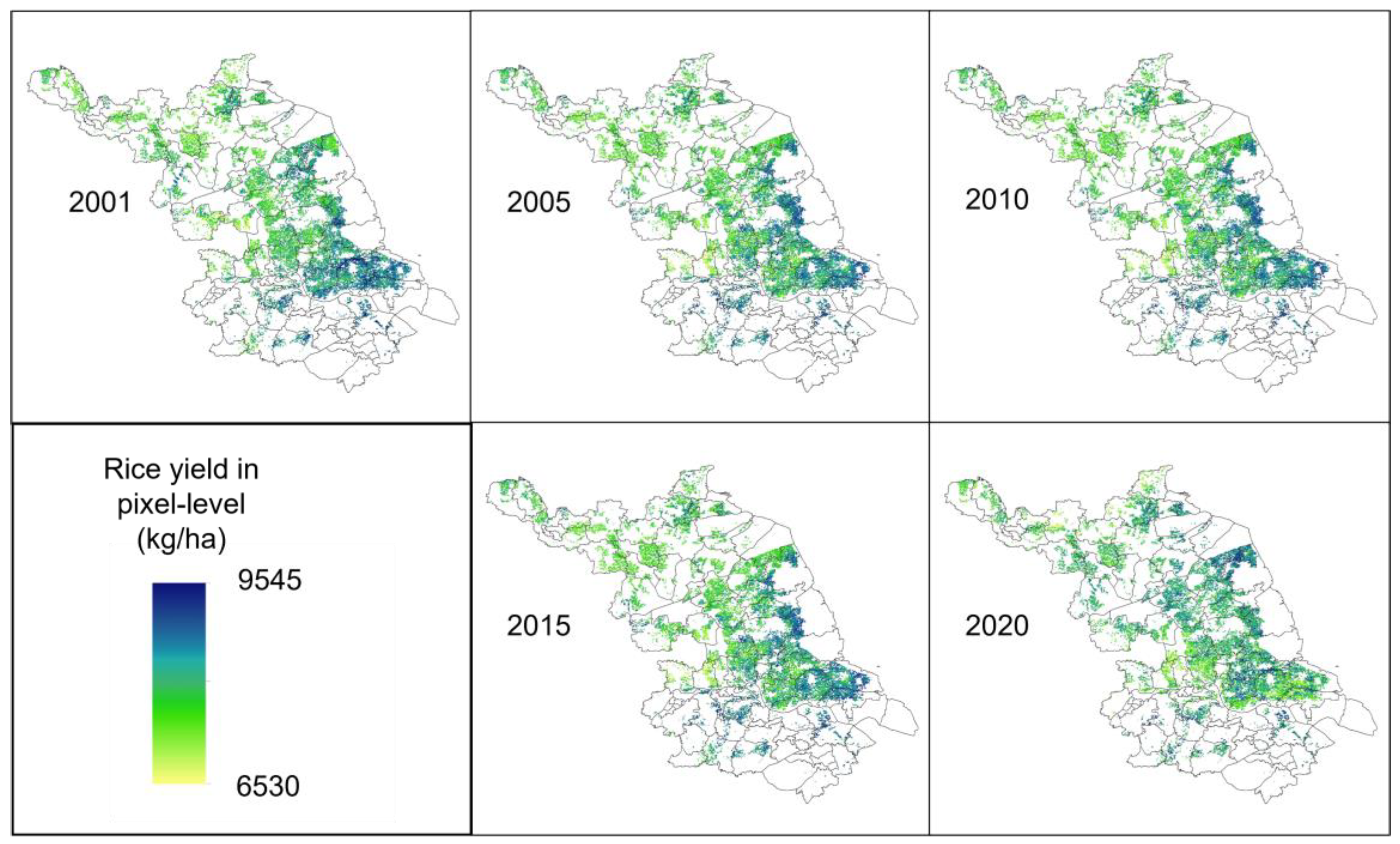
3.4. Pixel-Level Rice Yield Mapping

Understanding the spatial and temporal patterns of crop yields is fundamental for shaping agricultural policies. However, the data typically provided by statistical yearbooks, which are aggregated at the county level, lack the granularity necessary to capture more nuanced variations in crop yields. Remote sensing technology, on the other hand, offers high-resolution observations of the Earth’s surface, making it a valuable tool in this context. In this study, we leveraged the power of remote sensing to generate rice yield estimates for Jiangsu Province, China, covering the period from 2001 to 2020. Our approach involved using random forest regression with carefully selected NDVI data from seven key dates. As demonstrated in Figure 10, the resulting dataset offers an unprecedented level of detail, reflecting rice yield distributions at a resolution of 1 km. This high-resolution dataset holds significant potential for informing agricultural policy decisions and facilitating future research in related fields. Interested parties can access the dataset on the Zenodo database, where it has been made publicly available (DOI: 10.5281/zenodo.10719965).

4. Discussion

In contrast to single-date satellite observations of vegetation, continuous spatiotemporal remote sensing information provides a more thorough understanding of crop conditions [4,11,12,27]. By correlating rice yield with remotely sensed, multi-temporal phase NDVI values in this study, we effectively capture the dynamic changes in rice throughout its growth cycle using long time series remote sensing observations. Furthermore, this study demonstrates the feasibility and accuracy of machine-learning algorithms in predicting rice yield. Essentially, the integration of multi-temporal phase remote sensing data with machine-learning techniques enables precise rice yield estimates while maintaining excellent spatial applicability.

4.1. Comparation of Different Machine-Learning Algorithms

Previous studies have consistently emphasized that the relationship between crop yield and complex remote sensing information is not a straightforward linear one [17]. Consequently, linear regression algorithms, such as partial least squares regression (PLSR) or multiple linear regression (MLR), often struggle to manage the intricate multi-element integration challenges involved. This aligns with our study’s findings, which indicate a low accuracy for PLSR. In contrast, random forest regression (RFR) has proven to be adept at addressing complex nonlinear issues, providing a nuanced understanding of the underlying relationships [28]. Although back propagation neural networks (BPNN) have also demonstrated some capability in managing similar scenarios [13], they exhibited the lowest accuracy in estimating rice yield in our investigation. This might be attributed to the limited sample size available for model training. Previous research has established that neural network algorithms generally rely heavily on the volume of samples for effective training, and the few hundred samples utilized in this study might not have met the requirements of such algorithms [29]. Additionally, BPNN can be susceptible to outliers, which are inevitably present in rice yield data recorded in statistical yearbooks. On the other hand, RFR, a widely recognized ensemble machine-learning algorithm known for its excellent performance, leverages the bagging algorithm. It randomly selects samples and attributes from the dataset to build numerous classifiers, each voting to determine the final classification. This approach minimizes the impact of limited or abnormal samples, focusing more on the choice of key parameters, like the number of randomly selected attributes and the number of classifiers built [14]. Similarly, support vector regression (SVR) relies on a subset of samples, known as support vectors, for decision-making, reducing both computational complexity and the influence of outlier samples. However, SVR’s effectiveness is greatly dependent on the careful selection of parameters, such as the penalty coefficient and kernel function parameters, as different choices can lead to significantly different outcomes [10]. Overall, given the uncertainties inherent in recorded rice yield data and the accuracy of remotely sensed information, RFR, with its multiple parallel regression trees, is likely to yield more consistent and reliable results when compared to other machine-learning algorithms.

4.2. The Influence from the Model Inputs

In this study, NDVI data from 109 dates spanning the rice transplanting stage to maturity stage were chosen as inputs for a random forest regression (RFR) model to predict rice yield. Although the extensive remote sensing data offer comprehensive monitoring of rice throughout its growth cycle, the sheer volume of information introduces redundancy and adds layers of complexity to the model. To strike a balance, we employed an importance-ranking method that narrowed down the NDVI inputs to seven key dates (specifically, the 6th, 17th, 33rd, 44th, 71st, 90th, and 106th days after the rice transplanting stage). These carefully selected data points are evenly distributed across various growth stages, effectively capturing the rice’s growth patterns while minimizing data redundancy and simplifying the model. Nevertheless, limitations and challenges still exist with this approach.
(1) Despite being one of the most popular vegetation indices in use today, NDVI still faces certain limitations due to spectral saturation. This arises from its dependence on the reflectance difference between the near-infrared (NIR) and red bands. In regions with dense vegetation, the red band reflectance significantly diminishes, while the NIR band reflectance approaches a saturation point, leading to a plateau in NDVI values [30]. In this study, we observed rice NDVI values exceeding 0.8, potentially indicating spectral saturation. Prior research has suggested that enhanced vegetation indices, such as EVI, can mitigate spectral saturation effects [31,32]. Hence, future studies should consider exploring a wider range of vegetation indices.
(2) Uncertainties in model inputs can propagate into the accuracy of yield estimation. In this study, although the MOD09 product provides surface spectral reflectance data with spatiotemporal continuity (daily and 1 km resolution), the inevitable influence of cloud cover results in some missing information. Additionally, the Savitzky–Golay filtering method employed here carries a degree of inherent error, which can subsequently impact rice yield estimation [33,34]. Likewise, the phenology product used in this study also has a margin of error [23], potentially leading to incorrect identification of the NDVI period.

4.3. The Spatial Applicability of Proposed Model

The models employed in various studies demonstrate exceptional performance when processing specific spatial datasets. However, their effectiveness often diminishes when applied to broader regional data due to the absence of actual training data from the target regions. To address this challenge, our study incorporates the Moran Index, which aids in managing spatial heterogeneity and adapting to regional variations. Spatial heterogeneity encompasses disparities in moisture levels and agricultural practices, including irrigation and fertilizer use across regions. Therefore, when introducing variables into the model, it is crucial to consider these differences and the interconnections of spatial heterogeneity [35]. By utilizing NDVI data from multiple timeframes as model inputs, we can gain a more nuanced understanding of regional disparities. It becomes evident that as the number of input variables increases, so does their association with spatial heterogeneity, enhancing the model’s sensitivity to spatial information changes. Consequently, integrating multiple physiological indicators in rice yield estimation can enhance the proposed model’s accuracy and spatial versatility.

5. Conclusions

In this study, we employed four widely used machine-learning algorithms, partial least squares regression (PLSR), support vector regression (SVR), random forest regression (RFR), and back propagation neural network (BPNN), with multi-temporal rice NDVI data for rice yield estimation. After conducting accuracy evaluations and spatial analyses, our findings can be summarized as follows.
(1) The RFR model achieved the highest accuracy in rice yield estimation with an R2 value of 0.65, RMSE of 388.79 kg/ha, and rRMSE of 4.48%. Both PLSR and SVR demonstrated comparable, albeit inferior, accuracy compared to RFR.
(2) By selecting the top seven predictors with the highest importance rankings (NDVI values on the 6th, 17th, 33rd, 44th, 71st, 90th, and 106th days after the rice transplanting stage) as inputs for the RFR model, we achieved comparable accuracy while reducing information redundancy.
(3) Our proposed model exhibits good spatial applicability (MI = −0.03) for rice yield estimation in Jiangsu, China.
(4) Using the proposed model, we generated a high spatial resolution rice yield dataset (1 km) spanning from 2001 to 2020. This dataset is freely available on the Zenodo database (DOI: 10.5281/zenodo.10719965).
In general, this study has demonstrated the efficacy of combining multi-temporal remote sensing data with machine-learning techniques for accurate rice yield estimation. The predictions generated by this approach exhibit strong spatial adaptability, enabling them to effectively manage spatial variations arising from diverse cropping practices or environmental fluctuations across different regions. The findings underscore the reliability of satellite remote sensing data in yield prediction, thereby aiding agricultural authorities and production enterprises in the timely formulation and refinement of cropping strategies and management policies for the ongoing season. This, in turn, can offer valuable guidance for enhancing crop yields in various regions. Future research endeavors can further enhance the outcomes of this study by narrowing the temporal resolution of remote sensing imagery, focusing on pest infestations and natural disasters, and incorporating additional predictors to enhance the predictive accuracy and simplicity. Moreover, there is a need for further exploration into yield estimation for diverse crop types grown in distinct geographical locations.

Author Contributions

Methodology, Z.L. and M.C.; Software, Y.L. and M.C.; Validation, Z.L., H.J., Y.L., K.L. and T.W.; Resources, H.J., Q.M. and M.C.; Data curation, Q.M., T.W. and M.C.; Writing—original draft, Z.L. and K.L.; Writing—review & editing, C.S. and M.C. All authors have read and agreed to the published version of the manuscript.

Funding

This research was supported by the Basic Research Program Natural Science Foundation of Jiangsu Province (Grant No. SBK2023043261), National Natural Science Foundation of China (Grant No. 42301366), China Postdoctoral Science Foundation (Grant No. 2023M733001), and A Project Funded by the Priority Academic Program Development of Jiangsu Higher Education Institutions (PAPD).

Data Availability Statement

The data presented in this study are openly available in Zenodo database (DOI: 10.5281/zenodo.10719964).

Conflicts of Interest

The authors declare no conflicts of interest.

References

  1. Di, Y.; Gao, M.; Feng, F.; Li, Q.; Zhang, H. A New Framework for Winter Wheat Yield Prediction Integrating Deep Learning and Bayesian Optimization. Agronomy 2022, 12, 3194. [Google Scholar] [CrossRef]
  2. Kuenzer, C.; Knauer, K. Remote sensing of rice crop areas. Int. J. Remote Sens. 2013, 34, 2101–2139. [Google Scholar] [CrossRef]
  3. Gumma, M.K.; Mohanty, S.; Nelson, A.; Arnel, R.; Mohammed, I.A.; Das, S.R. Remote sensing based change analysis of rice environments in Odisha, India. J. Environ. Manag. 2015, 148, 31–41. [Google Scholar] [CrossRef]
  4. Li, L.; Wang, B.; Feng, P.; Wang, H.; He, Q.; Wang, Y.; Liu, D.L.; Li, Y.; He, J.; Feng, H.; et al. Crop yield forecasting and associated optimum lead time analysis based on multi-source environmental data across China. Agric. For. Meteorol. 2021, 308–309, 108558. [Google Scholar] [CrossRef]
  5. Fernandez-Ordoñez, Y.M.; Soria-Ruiz, J. (Eds.) Maize crop yield estimation with remote sensing and empirical models. In Proceedings of the 2017 IEEE International Geoscience and Remote Sensing Symposium (IGARSS), Fort Worth, TX, USA, 23–28 July 2017; IEEE: New York, NY, USA, 2017. [Google Scholar]
  6. Pettorelli, N.; Vik, J.O.; Mysterud, A.; Gaillard, J.-M.; Tucker, C.J.; Stenseth, N.C. Using the satellite-derived NDVI to assess ecological responses to environmental change. Trends Ecol. Evol. 2005, 20, 503–510. [Google Scholar] [CrossRef]
  7. Kogan, F.N. Application of vegetation index and brightness temperature for drought detection. Adv. Space Res. 1995, 15, 91–100. [Google Scholar] [CrossRef]
  8. Quiring, S.M.; Ganesh, S. Evaluating the utility of the Vegetation Condition Index (VCI) for monitoring meteorological drought in Texas. Agric. For. Meteorol. 2010, 150, 330–339. [Google Scholar] [CrossRef]
  9. Hu, X.; Ren, H.; Tansey, K.; Zheng, Y.; Ghent, D.; Liu, X.; Yan, L. Agricultural drought monitoring using European Space Agency Sentinel 3A land surface temperature and normalized difference vegetation index imageries. Agric. For. Meteorol. 2019, 279, 107707. [Google Scholar] [CrossRef]
  10. Maimaitijiang, M.; Sagan, V.; Sidike, P.; Hartling, S.; Esposito, F.; Fritschi, F.B. Soybean yield prediction from UAV using multimodal data fusion and deep learning. Remote Sens. Environ. 2020, 237, 111599. [Google Scholar] [CrossRef]
  11. Cheng, M.; Jiao, X.; Shi, L.; Penuelas, J.; Kumar, L.; Nie, C.; Wu, T.; Liu, K.; Wu, W.; Jin, X. High-resolution crop yield and water productivity dataset generated using random forest and remote sensing. Sci. Data 2022, 9, 641. [Google Scholar] [CrossRef]
  12. Cheng, M.; Penuelas, J.; McCabe, M.F.; Atzberger, C.; Jiao, X.; Wu, W.; Jin, X. Combining multi-indicators with machine-learning algorithms for maize yield early prediction at the county-level in China. Agric. For. Meteorol. 2022, 323, 109057. [Google Scholar] [CrossRef]
  13. Cheng, M.; Jiao, X.; Liu, Y.; Shao, M.; Yu, X.; Bai, Y.; Wang, Z.; Wang, S.; Tuohuti, N.; Liu, S.; et al. Estimation of soil moisture content under high maize canopy coverage from UAV multimodal data and machine learning. Agric. Water Manag. 2022, 264, 107530. [Google Scholar] [CrossRef]
  14. Yang, L.; Zhang, X.; Liang, S.; Yao, Y.; Jia, K.; Jia, A. Estimating Surface Downward Shortwave Radiation over China Based on the Gradient Boosting Decision Tree Method. Remote Sens. 2018, 10, 185. [Google Scholar] [CrossRef]
  15. Mojaddadi, H.; Pradhan, B.; Nampak, H.; Ahmad, N.; Ghazali, A.H.b. Ensemble machine-learning-based geospatial approach for flood risk assessment using multi-sensor remote-sensing data and GIS. Geomat. Nat. Hazards Risk 2017, 8, 1080–1102. [Google Scholar] [CrossRef]
  16. van Klompenburg, T.; Kassahun, A.; Catal, C. Crop yield prediction using machine learning: A systematic literature review. Comput. Electron. Agric. 2020, 177, 105709. [Google Scholar] [CrossRef]
  17. Cao, J.; Zhang, Z.; Luo, Y.; Zhang, L.; Zhang, J.; Li, Z.; Tao, F. Wheat yield predictions at a county and field scale with deep learning, machine learning, and google earth engine. Eur. J. Agron. 2021, 123, 126204. [Google Scholar]
  18. Huang, M. The decreasing area of hybrid rice production in China: Causes and potential effects on Chinese rice self-sufficiency. Food Secur. 2022, 14, 267–272. [Google Scholar] [CrossRef]
  19. Normile, D. Variety Spices Up Chinese Rice Yields. Science 2000, 289, 1122–1123. [Google Scholar] [CrossRef]
  20. Johnson, M.D.; Hsieh, W.W.; Cannon, A.J.; Davidson, A.; Bédard, F. Crop yield forecasting on the Canadian Prairies by remotely sensed vegetation indices and machine learning methods. Agric. For. Meteorol. 2016, 218–219, 74–84. [Google Scholar] [CrossRef]
  21. Jiang, Z.; Huete, A.R.; Chen, J.; Chen, Y.; Li, J.; Yan, G.; Zhang, X. Analysis of NDVI and scaled difference vegetation index retrievals of vegetation fraction. Remote Sens. Environ. 2006, 101, 366–378. [Google Scholar]
  22. Chen, J.; Jönsson, P.; Tamura, M.; Gu, Z.; Matsushita, B.; Eklundh, L. A simple method for reconstructing a high-quality NDVI time-series data set based on the Savitzky–Golay filter. Remote Sens. Environ. 2004, 91, 332–344. [Google Scholar]
  23. Luo, Y.; Zhang, Z.; Chen, Y.; Li, Z.; Tao, F. ChinaCropPhen1km: A high-resolution crop phenological dataset for three staple crops in China during 2000–2015 based on leaf area index (LAI) products. Earth Syst. Sci. Data 2020, 12, 197–214. [Google Scholar]
  24. Cheng, M.; Li, B.; Jiao, X.; Huang, X.; Fan, H.; Lin, R.; Liu, K. Using multimodal remote sensing data to estimate regional-scale soil moisture content: A case study of Beijing, China. Agric. Water Manag. 2022, 260, 107298. [Google Scholar] [CrossRef]
  25. Peralta, N.R.; Assefa, Y.; Du, J.; Barden, C.J.; Ciampitti, I.A. Mid-Season High-Resolution Satellite Imagery for Forecasting Site-Specific Corn Yield. Remote Sens. 2016, 8, 848. [Google Scholar] [CrossRef]
  26. Imran, M.; Stein, A.; Zurita-Milla, R. Using geographically weighted regression kriging for crop yield mapping in West Africa. Int. J. Geogr. Inf. Sci. 2015, 29, 234–257. [Google Scholar] [CrossRef]
  27. Li, Y.; Zhao, B.; Wang, J.; Li, Y.; Yuan, Y. Winter Wheat Yield Estimation Based on Multi-Temporal and Multi-Sensor Remote Sensing Data Fusion. Agriculture 2023, 13, 2190. [Google Scholar] [CrossRef]
  28. Chlingaryan, A.; Sukkarieh, S.; Whelan, B. Machine learning approaches for crop yield prediction and nitrogen status estimation in precision agriculture: A review. Comput. Electron. Agric. 2018, 151, 61–69. [Google Scholar] [CrossRef]
  29. Zhou, S.; Xu, L.; Chen, N. Rice Yield Prediction in Hubei Province Based on Deep Learning and the Effect of Spatial Heterogeneity. Remote Sens. 2023, 15, 1361. [Google Scholar] [CrossRef]
  30. Gitelson, A.A.; Kaufman, Y.J. MODIS NDVI optimization to fit the AVHRR data series—Spectral considerations. Remote Sens. Environ. 1998, 66, 343–350. [Google Scholar]
  31. Gu, Y.; Wylie, B.K.; Howard, D.M.; Phuyal, K.P.; Ji, L. NDVI saturation adjustment: A new approach for improving cropland performance estimates in the Greater Platte River Basin, USA. Ecol. Indic. 2013, 30, 1–6. [Google Scholar]
  32. Garroutte, E.L.; Hansen, A.J.; Lawrence, R.L. Using NDVI and EVI to map spatiotemporal variation in the biomass and quality of forage for migratory elk in the Greater Yellowstone Ecosystem. Remote Sens. 2016, 8, 404. [Google Scholar] [CrossRef]
  33. Cao, R.; Chen, Y.; Shen, M.; Chen, J.; Zhou, J.; Wang, C.; Yang, W. A simple method to improve the quality of NDVI time-series data by integrating spatiotemporal information with the Savitzky-Golay filter. Remote Sens. Environ. 2018, 217, 244–257. [Google Scholar]
  34. Chen, Y.; Cao, R.; Chen, J.; Liu, L.; Matsushita, B. A practical approach to reconstruct high-quality Landsat NDVI time-series data by gap filling and the Savitzky–Golay filter. ISPRS J. Photogramm. Remote Sens. 2021, 180, 174–190. [Google Scholar]
  35. Ray, S.S.; Dadhwal, V.K. Estimation of crop evapotranspiration of irrigation command area using remote sensing and GIS. Agric. Water Manag. 2001, 49, 239–249. [Google Scholar] [CrossRef]
Figure 1. Study area. Note: The rice planting area data are obtained from the Resource and Environment Science and Data Center, Chinese Academy of Science (http://www.resdc.cn).
Agriculture 14 00638 g001
Figure 2. The NDVI of rice variation after transplanting stage.
Agriculture 14 00638 g002
Figure 3. Distribution of recorded rice yield at county level: (a) histogram and (b) spatial distribution of the average value.
Agriculture 14 00638 g003
Figure 4. The flowchart of the rice yield estimation.
Agriculture 14 00638 g004
Figure 5. The scatter plot of rice yield estimation by different machine-learning algorithms: (a) BPNN; (b) PLSR; (c) SVR; and (d) RFR.
Agriculture 14 00638 g005
Figure 6. Correlation coefficient matrix of NDVI in rice at different stages.
Agriculture 14 00638 g006
Figure 7. Importance of NDVI at different stages.
Agriculture 14 00638 g007
Figure 8. Accuracy of rice yield estimation after excluded predictors: (a) R2 and (b) RMSE.
Agriculture 14 00638 g008
Figure 9. The average bias of proposed model in estimating rice yield at county level: (a) histogram and (b) spatial distribution of the bias.
Agriculture 14 00638 g009
Figure 10. The pixel-level rice yield in Jiangsu, China, based on the proposed model.
Agriculture 14 00638 g010
Disclaimer/Publisher’s Note: The statements, opinions and data contained in all publications are solely those of the individual author(s) and contributor(s) and not of MDPI and/or the editor(s). MDPI and/or the editor(s) disclaim responsibility for any injury to people or property resulting from any ideas, methods, instructions or products referred to in the content.

