Abstract
Current numerical methods for simulating biophysical processes in aquatic environments are typically constructed in a grid-based Eulerian framework or as an individual-based model in a particle-based Lagrangian framework. Often, the biogeochemical processes and physical (hydrodynamic) processes occur at different time and space scales, and changes in biological processes do not affect the hydrodynamic conditions. Therefore, it is possible to develop an alternative strategy to grid-based approaches for linking hydrodynamic and biogeochemical models that can significantly improve computational efficiency for this type of linked biophysical model. In this work, we utilize a new technique that links hydrodynamic effects and biological processes through a property-carrying particle model (PCPM) in a Lagrangian/Eulerian framework. The model is tested in idealized cases and its utility is demonstrated in a practical application to Sandusky Bay. Results show the integration of Lagrangian and Eulerian approaches allows for a natural coupling of mass transport (represented by particle movements and random walk) and biological processes in water columns which is described by a nutrient-phytoplankton-zooplankton-detritus (NPZD) biological model. This method is far more efficient than traditional tracer-based Eulerian biophysical models for 3-D simulation, particularly for a large domain and/or ensemble simulations.
1. Introduction
Current numerical methods for simulating biogeochemical processes in aquatic environments are typically constructed as individual-based models (IBMs) using Lagrangian particles [1,2,3] or as grid-based concentration models in an Eulerian framework [4,5,6]. IBMs allow for a mechanistic description of individuals and of interactions among individuals, represented by an ensemble of particles. Each individual contains a set of state variables (e.g., age, size, and nutrient quota) with corresponding physiological traits and behavioral traits [3], and the population-level properties emerge as a result of the cumulative behavior of the individuals [7]. IBMs have rapidly gained popularity in ecological modeling, particularly when simulating complete life cycles, adaptive behavior, and intrapopulation variability in response to internal and external environmental conditions becomes essential [8,9]. Large computational demand has long been known as one of the hallmark problems for IBM [2,7,8]. This is still true even with increased computational resources and implementation of the strategic approaches for reducing the number of individuals explicitly simulated in the model such as introducing the super individual particles or representative spaces [2].
On the other hand, the traditional grid-based Eulerian approach is also widely used in coupled physical–biogeological modeling [6,7,10,11] in the inland water and ocean modeling communities [12,13,14,15,16,17,18]. Unlike the particle models in which mass is transported as discrete particles [19,20], the Eulerian (concentration) model assumes average properties (state variables) of a population within a control volume, and estimates the change of the property using mass balance and reaction equations [21]. It does not describe intrapopulation variability but focuses on characteristics of the population mean, which is appropriate when growth kinetics are formulated as a function of the external conditions [7].
In general, the Eulerian model employs finite difference or finite element schemes to solve the governing reaction-transport equations [4,6]. Equations for the time evolution of state variables of the biophysical model include advection and diffusion terms which depend on hydrodynamic variables, as well as source and sink terms representing growth, decay, and interaction with other biogeochemical variables [6,11,22]. The property concentration fields () are often calculated using a set of advection–diffusion equations:
where D is the total water depth, and are the x, y, and components of the water velocity, is the vertical thermal diffusion coefficient, is the horizontal diffusion term, and and represents the sources and sinks of , respectively, due to the biological processes which are typically described using a set of biological process equations.
However, even in the relatively simple, less computationally demanding Eulerian model, a major practical challenge is that the biological submodel often involves a large group of parameters for calibration and confirmation which requires a considerable amount of computational time to tune the model. As shown in Equation (1), tuning the simulation of biological processes (e.g., changes in parameterization, initial and boundary conditions) requires a complete time integration of the entire equation, although bio-physical coupled models can have different time steps for physical and biological process terms as they may have different time and space scales. However, biophysical processes are generally not two-way coupled. In other words, one can often assume that changes in biological processes (in our case, the resulting changes in nutrient-phytoplankton-zooplankton-detritus (NPZD) property concentration) do not affect the hydrodynamic condition (currents, temperature, mixing, etc.). This indicates that there may be a more computationally efficient approach to resolve the impact of hydrodynamics on the biological processes rather than explicit integration of Equation (1) for each biological component every time the biological submodel is tuned.
The property-carrying particle model (PCPM) is developed to test the feasibility of an alternative strategy to grid-based approaches for linking hydrodynamic and biogeochemical models in the Eulerian framework that may reduce the problems mentioned above, particularly in regions where advection–diffusion plays a key role in regulating biogeochemcal processes. Instead of grid-based, time-averaging of hydrodynamic variables, the hydrodynamic model is used to calculate the Lagrangian trajectories of a large number of current-following tracer particles; these trajectories become the linking mechanism between the hydrodynamic model and the biogeochemical model. In the hybrid Lagrangian–Eulerian PCPM, each current-following tracer particle carries with it a number of time-varying properties which correspond to the state variables of the Eulerian biogeochemical model. The PCPM also employs its own horizontal grid system or series of regions which is independent of the hydrodynamic model grid and is used to calculate local average values of the particle-based properties. These cell-based properties allow all particles within a PCPM cell to influence the properties of other particles within the same cell or region and allow for display and analysis of biogeochemical fields. PCPM also differs from typical IBMs in that the tracer particles in PCPM typically carry ‘field’ based properties like concentration, as opposed to properties associated with an individual organism.
PCPM uses a computational grid system which is independent of the grid system used to compute currents for particle trajectories. The PCPM computational cells are used to define regions in which the properties carried by the particles are allowed to interact with one another. In this respect, PCPM is conceptually similar to the classic particle-in-cell (PIC) method with PM (particle–mesh) interactions [23,24], popularly used in plasma simulation [24,25]. PIC methods can also be mesh-independent by allowing direct particle–particle (PP) interactions, or a combination of PM and PP [23,24,25,26]. In PCPM, a basic simplifying assumption is that only particles within a single PCPM cell are allowed to interact, such as the PIC–PM method. The advantage of this approach is that it is conceptually intuitive to implement and computationally efficient to program.
An alternative approach to implementing a PCPM would allow particle-based properties to influence particle trajectories, perhaps through buoyancy or sinking. In this case, the PCPM would have to be coupled directly with the particle trajectory calculation. In the initial implementation of PCPM in this paper, we consider only the uncoupled case.
To illustrate more clearly the type of application envisioned for PCPM, we constructed and applied a rudimentary biophysical model to an actual aquatic system, Sandusky Bay, where the physical transport of flow and nutrient loading from the Sandusky River has proven to be critical to the ecosystem [27,28]. Since the mid-1990s, harmful algal blooms (HABs) have become the new norm for summer months in the Lake Erie ecosystem [29]. Harmful algal blooms occur in the system when cyanobacteria are provided the right temperature, light, and nutrient conditions to proliferate [30]. When these blooms transpire, they have many adverse impacts. At the local ecosystem level, HABs result in depleted dissolved oxygen levels below the lake’s surface threatening the survival of organisms living below the surface [31]. Additionally, some cyanobacteria species produce a toxin, such as microcystin, which affects the nervous system, liver, and kidney further impeding aquatic organisms and humans [31].
The colonial cyanobacterium Microcystis dominates the cyanobacterial community in the offshore waters of western Lake Erie; however, the filamentous cyanobacterium Planktothrix dominates the nearshore bays and tributaries [28], such as in Sandusky Bay [27,28,32]. Situated on Lake Erie’s south-western coast, Sandusky Bay borders Ohio’s Ottawa, Erie, and Sandusky counties (Figure 1). From a physical aspect, Sandusky Bay is relatively shallow bay with an average depth of roughly 2.6 m as well as occupying a relatively small area [32]. The primary draining watershed to Sandusky Bay originates from the Sandusky River at the west end of the bay. The Sandusky River drains a 1420 square mile area; of which, over 80% is dedicated to agricultural production [31]. This largely agricultural watershed leads to high nitrogen and phosphorus entering Sandusky Bay. Combining these high nutrient loads with the physical aspects leads to very high concentrations of nitrogen and phosphorus within Sandusky Bay, thus resulting in these cyanobacteria blooms (Planktothrix agardhii) [27,28,32].
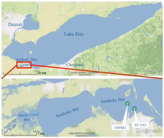
Figure 1.
Sandusky Bay is situated on Lake Erie’s south-west coast occupying a small portion of the Great Lake’s coastline. Sandusky Bay is relatively shallow bay with an average depth of ~2.6 m. The primary draining watershed to Sandusky Bay originates from the Sandusky River on the west end of the bay. Sampling stations ODNR1 and EC1163 are denoted with green dots.
The intent of this study is to test the feasibility of PCPM for biological–physical coupled modeling and examine its effectiveness and computational efficiency in practical application by implementing it in relation to HABs in Sandusky Bay. The remaining sections of this paper are organized as follows: details of PCPM and the design of numerical experiments are described in Section 2. The model results of idealized cases and the practical application to Sandusky Bay are presented in Section 3. A discussion and summary of the PCPM applications are included in Section 4.
2. Methods
2.1. Property-Carrying Particle Model (PCPM)
In this implementation of PCPM, particle trajectories are pre-computed based on the output of a hydrodynamic model and are independent of the particle properties. An initial particle density (i.e., total number of particles/volume of computational domain) is selected and particles are randomly distributed throughout the computational domain. Particles are not allowed to leave the computational domain except at hydrodynamic outflows. At hydrodynamic inflows, new particles are introduced with the same density as the initial distribution. The total number of active particles is not strictly preserved, but if there is a net balance of hydrodynamic inflows and outflows, the total number of particles is approximately constant.
Any suitable method can be used to generate the Lagrangian particle trajectories. Typically, the trajectories are calculated from a time integration of the Lagrangian equations of motion:
where (x, y, z) is the particle’s position in 3 dimensions, (u, v, w) is the local fluid velocity vector, and t is time. For the two idealized examples presented in this paper, the trajectories are calculated semi-analytically from a simple, idealized flow field. The third, more realistic example, demonstrates the use of a full hydrodynamic model of a natural basin (i.e., Sandusky Bay) to compute currents and trajectories.
Each computational time step in the PCPM consists of six intermediate steps:
- Read particle locations (x, y, z) and temperature. This step simply updates the location of each particle that is being used in the computation. Figure 2 is a conceptual representation of a PCPM computational cell, Particles (m1, m2, m3,…) move in and out of the cell at each PCPM time step based on their trajectories as computed from the hydrodynamic model. The total number of particles for a particular computation is assumed to be fixed for the duration of the computation, although some particles may enter or leave the PCPM domain during the computation. Water temperature or other physical properties from the hydrodynamic calculation can be stored along with the pre-computed particle trajectories and can be included as one of the properties (P1, P2, P3, …) carried by the particle.
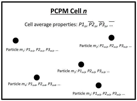 Figure 2. Conceptual representation of a property-carrying particle model (PCPM) computational cell n and particles (m1, m2, m3, m4, m5…) within the cell n. PCPM cell-based average of each property (, , ,…) is determined by the property values carried by the particles that have entered in this cell. After time evolution of PCPM properties using process equations, the updated PCPM cell-based properties (, , ,…) are redistributed to particles with a weighted average. The particles then move around carrying the updated properties to different PCPM computational cells in the next cycle.
 - Determine the PCPM cell for each particle. In Figure 2, the PCPM cell is represented by the enclosing rectangle. The PCPM domain need not coincide with the domain that was used for the hydrodynamic simulation and computation of particle trajectories. It can be regular or irregular, as long as there is a prescribed method to calculate which PCPM cell contains a prescribed particle position (x, y, z). The PCPM cells are the volumes within which particle properties can interact, that is, during a single time step, all particles within a PCPM cell can influence the evolution of particle properties within that cell, but are independent of other cells.
- Apply boundary conditions to any particle-based properties that require them. If there is a property (e.g., concentration of a dissolved nutrient) that needs to be specified as a boundary condition, then particles within the cell where the boundary condition needs to be applied will have that property adjusted to meet the boundary condition. For example, in a cell that is associated with an inflow to the domain, the properties that are being carried into the domain through the inflow are adjusted to take account of the change in that property for particles within that cell. Alternatively, if particles from the hydrodynamic-based trajectory calculation are entering a PCPM cell, the values of the associated properties for each particle need to be specified.
- Calculate PCPM cell-based averages of each property. In this step, the averages of property for cell n are calculated as:where the summation includes all particles (m1, m2,...) currently within cell n. L is the number of particles within that cell. If no particles are present in a particular cell, PCPM uses the values of from the previous time step.
- Calculate the time evolution of the cell-based properties (and particle-based properties if necessary) using the process equation defined for that property. The process equations can incorporate terms which depend on either particle-based or cell-based properties, or both, i.e.,Note that M indicates m1, m2,.... The form of FN is completely general and depends on the problem being solved. For instance, in a NPZD model, the ) would be N, P, Z, D, and water temperature, and the FN would be the process equations relating these properties.Since the cell-based averages have already been computed, the right-hand side of Equation (4) is independent of the left-hand side, so the computation of the evolution equations can be carried out in parallel. This is another key design feature of PCPM allowing it to take full advantage of multiprocessing computer environments, both symmetric multi-processing (SMP) and massively parallel processing (MPP).
- Redistribute cell-based properties to particles within each cell by replacing the particle-based property with a weighted average of the cell-based property. After the evolution equations have been carried out (Step 5), particles within an individual cell most likely carry a range of different values of the various properties, which vary around the new cell-based average computed in Step 5, . PCPM provides an optional step to reduce the variance of the new particle-based properties within each cell. This optional step is applied as a ‘nudging’ term, i.e.,where 0 < < 1 is the redistribution weight (i.e., nudging) factor. If = 0, no adjustment is carried out and the particle-based property remains unchanged. If = 1, then all particles within a cell are assigned the cell-based average of that property. This step can be useful to smooth results when limited particle density results in excessive within-cell variability.
Note that all steps except 3 and 5 are independent of the specific problem, i.e., they will be carried out the same way no matter how many properties are attached to the particles or what those properties represent. More importantly, steps 1 and 2 only need to be run once regardless of modifications in biological processes at the later stage. These are two of the key designs of PCPM that contribute to enhanced computational efficiency.
2.2. Idealized Case 1: Advection–Diffusion Plume
In PCPM, diffusion is provided mainly by particle trajectories, although the cell-based averaging of particle properties and the (optional) redistribution of cell-based properties to particles within the cell can also act as diffusive terms. To demonstrate the effect of particle trajectory diffusion on particle properties, we constructed a 500 m wide × 2000 m long channel divided into 10 m square cells. Particles were introduced at random locations along the center 400 m section of the left edge of the channel at the rate of 100/s. The particles were assigned an along-channel velocity of 2 m/s. Horizontal diffusion was added using a random-walk perturbation to the particle trajectories of in both cross-channel and long-channel directions. Here, is a uniformly distributed random number in the range [−1, 1], is the horizontal diffusion coefficient (10 m2/s in this experiment), and is the time step for the particle trajectory calculation (1 s).
In this example, PCPM particles carry only one property, concentration (P1 = C), and there is no time evolution equation (step 5, above). The purpose of this example is to illustrate how PCPM simulates horizontal diffusion through a combination of the particle trajectories and the cell-based averaging in step 6. To simulate a concentration plume, particles introduced in the center of the left wall (−50 m < y < 50 m) are assigned the initial condition C = 1. Particles entering the channel outside this region have an initial condition of C = 0.
2.3. Idealized Case 2: Vertical Settling
Since this implementation of PCPM does not allow the properties carried by the particles to influence particle trajectories, the question arises of how to simulate the vertical transport of a property when the vertical transport depends on the property itself, such as sediment settling or biologically generated buoyancy. In PCPM, the answer is simply to solve the vertical transport at the PCPM cell-based Eulerian framework in step 5 as a traditional cell-based method. Interaction of particle properties with adjacent cell averages is technically not allowed in the basic PCPM framework, but an exception is made in this case. The vertical advection–diffusion equation for sediment concentration is shown below:
where is the bulk settling velocity of the suspended material and is the vertical diffusion coefficient.
Since vertical diffusion is already included in the particle trajectories, PCPM only needs to consider the first term on the right-hand side of (7) to account for the additional vertical transport that depends on the property itself. To implement this term in the PCPM, the process equation for a particle carrying a property Cm in vertical cell k looks like:
where is the average concentration in vertical cell k, is the average concentration in the next higher vertical cell, and is the spacing between the centers of the cells. For particles in the top cell (k = 0), we set:
and for particles in the bottom cell (k = kmax), we set:
As a test case, we examine the vertical settling in a one-dimensional water column of depth d with particles moving vertically only through vertical diffusion. Particles are initially distributed randomly in the column and then move with a random walk velocity of where is a uniformly distributed random number in the range [−1, 1] and is the vertical diffusion coefficient. Particles are not allowed to cross the surface or bottom boundaries. Thus, in this experiment, the number of particles is constant and the particles are always approximately uniformly distributed in the vertical due to vertical mixing.
For the experiment, we set C = 1 as the bottom boundary condition by assigning this value at the beginning of each time step to all particles in the lower half of the bottom cell. The initial condition in other cells is C = 0. For the test case, we set the number of particles to 1000, d = 20 m, = 10−4 m2s−1, and the redistribution parameter α = 0.1. Three runs were made with 5, 10, and 20 vertical cells respectively. The PCPM is integrated in time with = 1 h.
2.4. Sandusky Bay Model
The hydrodynamic model used in this study is FVCOM (finite volume community ocean model) [33]. FVCOM is an unstructured-grid, finite-volume, three-dimensional (3-D) primitive equation ocean model with a generalized, terrain-following coordinate system in the vertical and a triangular mesh in the horizontal. The unstructured grid can be designed to provide a customized variable resolution to both coastline and bathymetry. With the merits of ideal geometric fitting and local refinement of mesh resolution, FVCOM has been used in numerous applications to estuaries, coastal oceans, and the Great Lakes [34,35,36,37,38,39,40]. These characteristics make the model well suited for the study of Sandusky Bay.
Although this study focuses on Sandusky Bay, FVCOM is configured to simulate physical dynamics for all of Lake Erie including a high-resolution Sandusky Bay-FVCOM developed in this study, thus providing reliable representation of large-scale background circulation and the role of remote forcing impacting the water movement in the bay through the opening; additionally, this configuration avoids the impact of setting an artificial numerical boundary condition for our target region. The hydrodynamic model is well calibrated for the Lake Erie, based on the next-generation National Oceanic and Atmospheric Administration (NOAA) Lake Erie Operational Forecast System (LEOFS; see Kelley et al., [40] for detailed model validation), a real-time nowcast and forecast model that is built on the FVCOM. In the upgraded NOAA operational model for Lake Erie [40], the FVCOM model is developed with horizontal resolution ranging from 100 to 2500 m, and 21 uniform vertical sigma (terrain-following) layers for Lake Erie. The advantage of our model setting is that model resolution varies from 100–2500 m (coarse) in the open lake to 10–50 m (fine) in Sandusky Bay, affording a high degree of resolution across the 20 km × 3 km study site and adequately resolving the geographic complexity and coastal hydrodynamic conditions of that system (Figure 3). The model configuration yields a total of 73,000 grid elements (cells) in the horizontal plane with 50,000 of them resolving the bay.
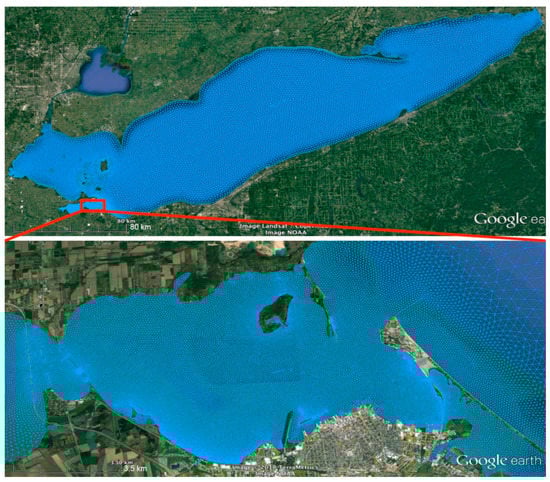
Figure 3.
Finite volume community ocean model (FVCOM) model mesh for Lake Erie (upper panel) and linked with a high-resolution mesh for Sandusky Bay (lower panel). Only a portion of the Sandusky Bay mesh is displayed for a clear representation of the mesh’s resolution.
In the PCPM implementation, 86,000 initial particles are randomly distributed throughout Sandusky Bay with a total water volume of 3.01 × . With PCPM cell resolution of 200 m × 200 m and the mean water depth of 2.6 m in Sandusky Bay, each PCPM cell contains 30 particles on average. New particles are introduced from the Sandusky River with the same density as the initial distribution. The number of new particles released from the river mouth varies greatly in accordance with the river flow rate. Table 1 presents the number of new particles released each month, based on the total water volume input from the Sandusky River. For example, 205,367 particles are released in March due to the highest river discharge in this month, which approximately equals the total number of particles (207,050) released from April to October.

Table 1.
The number of new particles released and the total water volume input from the Sandusky River in each month.
2.5. Sandusky Bay Biological Model
The biological model used in this work is a general 3-D NPZD model [17]. As a common approach, the biological model is constructed by implementing 1-D NPZD models for each vertical column of PCPM cells that are distributed spatially across the 2-D domain to form a 3-D representation of the system. An exchange of properties between adjacent water columns occurs across their shared interface through advection and dispersion. Figure 4 displays the interactions among state variables in the NPZD model.
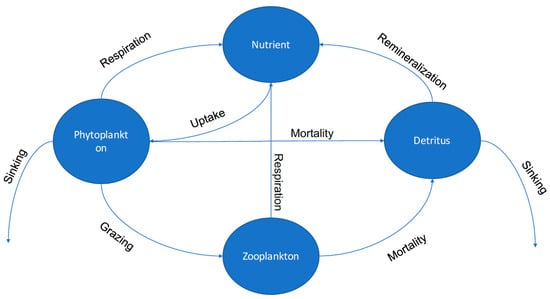
Figure 4.
A schematic representation of the nutrient-phytoplankton-zooplankton-detritus (NPZD) model.
The governing equations for the model framework are based on Luo et al. [17], and the mathematical expressions for each term of the system of Equations (10) is presented in Appendix A. Several equations in the governing equations are modified for this study based on literature review. The light-limited, nutrient-limited, and temperature-limited functions , respectively, that contribute to the are taken from Platt et al. [41] and Nicklisch et al. [42]. Also, the light attenuation functions are adjusted to Rowe et al. [18].
where , are the initial linear slope at low irradiance and the negative slope at the high irradiance that characterizes photoinhibition [43], is the maximum potential growth rate, and is the light intensity. The nutrient threshold represents the pool of nutrient that was assumed to be biologically unavailable. and are the optimal growth temperature and minimal growth temperature, respectively. is the light attenuation coefficient that accounts for the impact of water turbidity, phytoplankton, and detritus on the light attenuation. Model parameterization is based on literature review [17,18,41,43] and subjective tuning for the Sandusky Bay simulation as there is no established NPZD model for the Sandusky Bay region. (See Table 2 for model parameterization).
Table 2.
The comparison of total run time using the method developed in this study (new method) and the grid-based Eulerian method (traditional method) in two scenarios. Scenario 1: conduct coupled biophysical model only once; Scenario 2: run ensemble simulation of the coupled biophysical model for 100 simulations with different biological parameterization.
3. Results
3.1. Idealized Case 1: Advection–Diffusion Plume
To illustrate the effect of the cell-based averaging (step 6), we show results of the first idealized case for four different values of the cell-based redistribution parameter ( = 0, 0.01, 0.1, 0.5) in Figure 5. In Figure 5, there are three panels for each value of . The top panel shows the locations of particles after 720 time steps (12 min). The particles are colored using a blue-to-red scale for concentration values from 0 to 1. Particles with a concentration value of exactly 0 are colored light gray. The second panel shows the average concentration in each 10 m square cell with the same blue to red scale as the top panel, except cells with C = 0 are black. The third panel compares concentration along the centerline of the plume from the second panel to the analytical solution for a diffusive plume [44,45], i.e.,
where is the centerline concentration meters away from the channel entrance. represents Gauss error function, defined as: . In the case , there is no cell-based redistribution of properties, so all particles retain their initial concentration values of either C = 0 (light gray in panel 1) or C = 1 (red in panel 1). As seen in the second and third panels, the random-walk diffusion in the particle trajectories does provide a rough approximation to the analytical solution by mixing of C = 0 and C = 1 particles in the PCPM cells. Of course increasing the number of particles in the simulation would provide a more accurate approximation, but would also increase the computational load. Setting the cell-based redistribution parameter to even the small value of = 0.01 provides a significant improvement in the solution with the same number of particles, particularly for x > 500 m. Now particles can have any value of C between 0 and 1. Increasing the redistribution parameter to = 0.1 further improves the solution for x < 500 m. Further increasing to 0.5 does not significantly improve the solution in comparison to = 0.1.
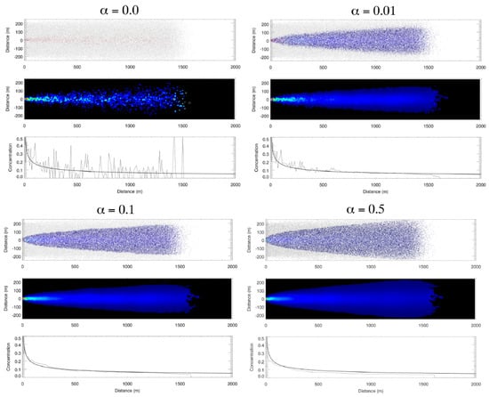
Figure 5.
PCPM simulation of concentration plume in an idealized channel with four different values of the cell-based redistribution weight parameter (α = 0, 0.01, 0.1, 0.5). There are three panels for each value of α. The top panel shows the locations of particles after 720 time steps (12 min). The second panel shows the average concentration in each 10 m square cell with the same blue to red scale as the top panel, except cells with C = 0 are black. The third panel compares concentration along the center line of the plume from the second panel to the analytical solution for a diffusive plume.
3.2. Idealized Case 2: Vertical Settling
The results at the end of 5000 time steps of the second idealized case are shown in Figure 6. In Figure 6, the dots represent the locations of the particles on the vertical axis and the value of concentration they are carrying on the horizontal axis. The thin line is the cell average concentration. The thick line is the analytical solution,
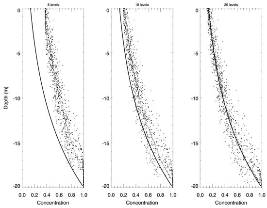
Figure 6.
The PCPM simulation of vertical settling in comparison to the analytical solution at the end of 5000 time steps. Three runs were made with 5 (left panel), 10 (middle panel), and 20 (right panel) vertical cells, respectively. The dots represent the locations of the particles on the vertical axis with their respective concentration on the horizontal axis. The thin line represents the cell average concentration and the thick line represents the analytical solution.
As shown in Figure 6, the model properly simulates the change in concentration due to vertical settling and mixing while allowing the particles to remain approximately uniformly distributed in the vertical. The simulation accuracy increases with increased resolution of vertical layers. The model result with 20 vertical layers shows a close agreement with the analytical solution. Specifically, Figure 7 shows the evolution in time of the root mean square difference (RMSD) between the cell averages and the analytical solution for the three cases. While the RMSD in the simulation with 5 layers remains above 0.2 (the magnitude of initial error) over the entire simulation, the RMSD decreases quickly to 0.02 after 500 time steps and remains stable at this level when vertical resolution is increased to 20 layers.
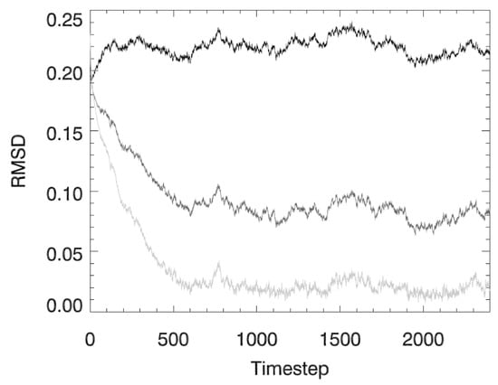
Figure 7.
The time evolution of the root mean square difference (RMSD) between the cell averages and the analytical solution for the three cases presented in the Figure 3 (dark line for 5 cells, medium line for 10 cells, and light line for 20 cells).
3.3. Application to Sandusky Bay
To ensure the validity of the 1-D NPZD biological model, it was configured to duplicate several scenarios (not shown) from Edwards et al. [46]. The model demonstrated the expected linear stability of a vertically-distributed, NPZ ecosystem model when it was used in the scenarios that incorporate the impact of vertical mixing on biological dynamics. Scenarios include stable profiles, damping oscillatory dynamical trajectories, and vertically phase-locked systems, depending on the depth and choice of parameters and strength of vertical diffusion, which can be discerned from the eigenvalues in linear stability analysis [46]. The 1-D NPZD model used in this study reproduced all of these cases almost identically.
Before examining the impact of physical transport on the biological dynamics in Sandusky Bay, we first tested the ability of PCPM to simulate the advection–diffusion using a conservative soluble tracer in a natural setting. The Sandusky River plume is simulated using the conventional soluble-tracer model based on the advection-diffusion equation and compared to the result of PCPM approach in Figure 8. It is clear that the plumes simulated using the two methods show a very similar pattern, indicating the validity of the PCPM. Upon closer review, the plume simulated with soluble-tracer model shows a smoother evolution and sharper gradient near the plume front. We speculate this is partly due to the constant random-walk scale (10 ) used in the current particle-tracking model configuration. Nonetheless, the attractiveness of PCPM is its computational efficiency; it runs ~100 times faster than the soluble-tracer model which will be discussed in detail in the following section and Table 2.
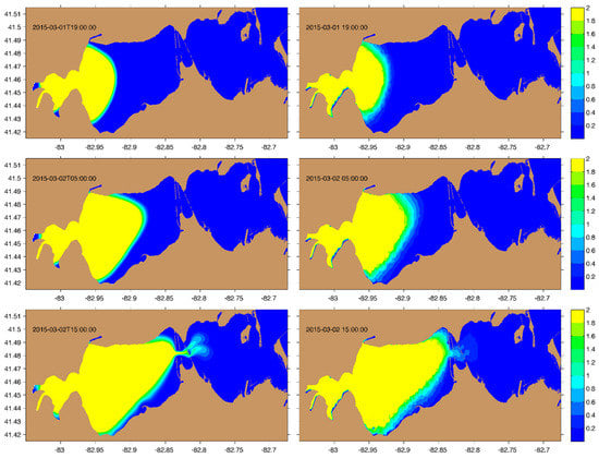
Figure 8.
River plumes at selected times (labelled in each panel) simulated with conventional soluble-tracer model (left panels) and PCPM model (right panels). The color scale represents the tracer concentration.
To aid in model development, several datasets are gathered from literature as well as data acquisition organizations. Sandusky River daily discharge and nitrogen concentration are available from the National Center for Water Quality Research (https://ncwqr.org/monitoring/data/, accessed on 12 July 2018). Nitrogen, Chlorophyll concentration, and in-situ temperature data are available from two observational sites (ODNR1 and EC1163) in the eastern bay from May–October 2015, sampled by Bowling Green State University [28].
Using the PCPM-NPZD model, the importance of physical transport is demonstrated by comparing model results between the PCPM-NPZD-NOADV (no advection) simulation and the realistic PCPM-NPZD-REAL simulation. In the PCPM-NPZD-NOADV simulation, the model is configured the same as the PCPM-NPZD-REAL, except the movement of particles is driven only by turbulent diffusion without including advective processes due to the Sandusky River and wind field. Each simulation consists of three cases that use a high initial nutrient concentration of 9 mg N/L in June (case 1), medium initial concentration of 0.46 mg N/L averaged from July to September (case 2), and low initial concentration of 0.0075 mg N/L in August (case 3), respectively. The concentration values are estimated as total nutrient loading from the Sandusky River to the Bay (https://ncwqr.org/monitoring/data/, accessed on 12 July 2018) divided by the total water volume of the bay. The comparison of model results is presented in Figure 9. The simulation of PCPM-NPZD-NOADV without resolving the advective transport processes shows a significant discrepancy from observational data (Figure 9, upper panels). The model fails to capture both the timing and magnitude of the blooms in all three cases, and model results are sensitive to the initial nutrient concentration.
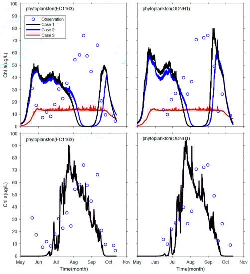
Figure 9.
Observed and model simulated chlorophyll concentration at the sampling stations EC1163 (left panels) and ODNR1 (right panels). The upper panels are results from the PCPM-NPZD-NOADV (no advection) model simulations; the lower panel are the results from the realistic PCPM-NPZD model simulations where the three cases show nearly identical results, so only one result is plotted.
On the other hand, after the impact of advective processes is resolved in the PCPM-NPZD-REAL simulation, the model accurately depicts the magnitude of the chlorophyll peak in mid-August (Figure 9, lower panels), and model results are insensitive to the initial condition, but determined by Sandusky River discharge and its nutrient loading. Three cases show nearly identical results. Results also support the field sampling study in Salk et al. [28]. Their study finds a strong, non-linear connection between the bloom occurrence and the hydraulic residence time of the bay, which varies dramatically from 8 days to several months depending on the Sandusky River flow rate in the physical transport process. Although further development of the NPZD is undoubtedly necessary to resolve the onset and variability of the algal blooms by refining the structure of the biological model and improving the model parameterization, it is beyond the scope of this work in which we focus on demonstrating the feasibility of linking hydrodynamic effects and biological processes through the PCPM in a Lagrangian/Eulerian framework. Further development of the biological model and its application to the study of mechanisms responsible for the HABs in Sandusky Bay will be presented in another paper.
4. Summary and Conclusions
In this paper, we describe a novel method by integrating a property-carrying particle model (PCPM) and an Eulerian concentration biological model for ecosystem modeling. The model is tested in idealized cases and its utility is demonstrated in a practical application to Sandusky Bay. The novelty of this new technique lies in its integration of hydrodynamic effects via the property-carrying particle tracking model and Eulerian grid-based biological modeling approach. Overall, there are several advantages of the PCPM over traditional Eulerian-based tracer approaches. The PCPM is simpler to implement and more efficient as it does not need to solve the advection–diffusion equation. Instead, the PCPM uses pre-computed particle trajectories to resolve the hydrodynamic condition based on currents from a hydrodynamic model. This means that the hydrodynamic model only needs to be run once giving one the ability to run different biological scenarios for the same physical characteristics; ultimately saving significant computational time.
As summarized in Table 2, a 30-day hydrodynamic simulation for the Lake Erie–Sandusky Bay FVCOM model takes 15 h to complete using 64 central processing units (CPUs). This step is necessary for both the PCPM-NPZD model and the traditional Eulerian, grid-based biophysical model. Once the hydrodynamic simulation is complete, PCPM-NPZD needs to calculate the Lagrangian trajectories of a large number of current-following tracer particles; it takes 1.5 h using a single CPU to track ~290,000 particles in the domain in March, which tracks the largest number of particles in the bay within a single month. The PCPM-NPZD model simulation using the particle trajectories as input completes a 30-day simulation within 5 min using a single CPU while it takes 5 h for a traditional Eulerian, grid-based biophysical model to complete the same simulation using 32 CPUs. If compared with the same computational power (e.g., single CPU), the PCPM-NPZD approach runs ~100 times faster for the biophysical modeling (Table 2; Scenario 1).
More importantly, in the PCPM framework, the hydrodynamics and associated water transport and mixing represented by particle trajectories are “reserved” and not affected by biochemical properties. In other words, it only takes another 5 min to run the PCPM-NPZD for a different set of parameters and property configurations. This is extremely useful during the model calibration and or ensemble simulations. The PCPM-NPZD would take 11.5 h to complete 100 runs using a single CPU, while the traditional method would require 500 h simulation using 32 CPUs (Table 2; Scenario 2). Such a high level of efficiency is not available from tracer-based models because one will have to re-run the Eulerian-based biological model for any change in parameter configuration or estimation of different property concentration. Also, the PCPM is capable of providing comparable simulation results to the soluble-tracer model, although the global and local mass conservation is not strictly preserved with finite particles. Above all, it is the PCPM’s computational efficiency and coupling flexibility which makes it an attractive alternative method to the traditional approach.
Author Contributions
Conceptualization, P.X. and D.J.S.; Formal analysis, X.Z., C.H., R.K. and X.Y.; Project administration, P.X.; Validation, X.Z.; Visualization, X.Z., C.H. and X.Y.; Writing—original draft, P.X. and D.J.S.; Writing—review and editing, P.X., D.J.S., R.K.
Funding
Xue’s work is partly supported by the Ohio Department of Natural Resources, Sandusky Bay Initiative.
Acknowledgments
This is the contribution 57 of the Great Lakes Research Center at Michigan Technological University. The Michigan Tech high performance computing cluster, Superior, was used in obtaining the modeling results presented in this publication. We thank George Bullerjahn, Robert McKay and Timothy Davis (Bowling Green State University) for access to their Sandusky Bay water quality data.
Conflicts of Interest
The authors declare no conflict of interest.
Appendix A
Table A1.
Biological model formulation and parameters; the original value of the parameters is provided in ( ) if tuned value was used.
Table A1.
Biological model formulation and parameters; the original value of the parameters is provided in ( ) if tuned value was used.
| Parameters | Description | Units | Value Used | References |
|---|---|---|---|---|
| Half-Saturation constant | µmol N/L | 3 (0.6) | [17] | |
| Nutrient threshold | µmol N/L | 0 (1.4) | [18] | |
| Initial linear slope at low irradiances | 7 | [18] | ||
| Negative slope at high irradiances | 0 | [43] | ||
| Maximum potential growth rate | 2.4 | [43] | ||
| Optimum temperature | °C | 27.2 | [42] | |
| Minimum temperature | °C | 5.5 | [42] | |
| Maximum growth rate for P | day−1 | 1.1 | ||
| Phytoplankton respiration coefficient | day−1 | 0.01 | [17] | |
| Exponential for Temperature forcing | dimensionless | 0.07 | [17] | |
| Remineralization rate of detritus | day−1 | 0.015 | [17] | |
| Maximum P grazing rate by Z | day−1 | 0.4 | [17] | |
| Preference coefficient of Z on P | 0.5 | [17] | ||
| Preference coefficient of Z on D | 0.1 | [17] | ||
| Mortality rate of P | day−1 | 0.005 (0.01) | [17] | |
| Mortality rate of Z | day−1 | 0.2 (0.01) | [17] | |
| Sink velocity of P | m/day | 0.6 | [17] | |
| Sink velocity of D | m/day | 0.6 | [17] | |
| Water attenuation coefficient | m−1 | 0.07 | [18] | |
| Phytoplankton attenuation coefficient | 0.03 | [18] | ||
| Detritus attenuation coefficient | 0.2 | [18] |
The mathematical expressions for the biological terms in the system of Equation (10) are listed below, where the definition and value of each parameter in the equations is above.
References
- Woods, J.D. The Lagrangian Ensemble metamodel for simulating plankton ecosystems. Prog. Oceanogr. 2005, 67, 84–159. [Google Scholar] [CrossRef]
- Hellweger, F.L.; Bucci, V. A bunch of tiny individuals—Individual-based modeling for microbes. Ecol. Model. 2009, 220, 8–22. [Google Scholar] [CrossRef]
- DeAngelis, D.L.; Grimm, V. Individual-based models in ecology after four decades. F1000prime Rep. 2014, 6, 39. [Google Scholar] [CrossRef] [PubMed]
- Chapra, S.C. Surface Water-Quality Modeling; McGraw-Hill: Boston, MA, USA, 1997. [Google Scholar]
- Franks, P.J. NPZ models of plankton dynamics: Their construction, coupling to physics, and application. J. Oceanogr. 2002, 58, 379–387. [Google Scholar] [CrossRef]
- Butenschön, M.; Clark, J.; Aldridge, J.N.; Allen, J.I.; Artioli, Y.; Blackford, J.; Lessin, G. ERSEM 15.06: A generic model for marine biogeochemistry and the ecosystem dynamics of the lower trophic levels. Geosci. Model Dev. 2016, 9, 1293–1339. [Google Scholar] [CrossRef]
- Hellweger, F.L.; Kianirad, E. Individual-based modeling of phytoplankton: Evaluating approaches for applying the cell quota model. J. Theor. Biol. 2007, 249, 554–565. [Google Scholar] [CrossRef] [PubMed]
- Hellweger, F.L.; Kravchuk, E.S.; Novotny, V.; Gladyshev, M.I. Agent-based modeling of the complex life cycle of a cyanobacterium (Anabaena) in a shallow reservoir. Limnol. Oceanogr. 2008, 53, 1227–1241. [Google Scholar] [CrossRef]
- Grimm, V.; Berger, U.; DeAngelis, D.L.; Polhill, J.G.; Giske, J.; Railsback, S.F. The ODD protocol: A review and first update. Ecol. Model. 2010, 221, 2760–2768. [Google Scholar] [CrossRef]
- Bruggeman, J.; Bolding, K. A general framework for aquatic biogeochemical models. Environ. Model. Softw. 2014, 61, 249–265. [Google Scholar] [CrossRef]
- Chai, F.; Dugdale, R.C.; Peng, T.H.; Wilkerson, F.P.; Barber, R.T. One-dimensional ecosystem model of the equatorial Pacific upwelling system. Part I: Model development and silicon and nitrogen cycle. Deep Sea Res. Part II Top. Stud. Oceanogr. 2002, 49, 2713–2745. [Google Scholar]
- Fennel, K.; Wilkin, J.; Levin, J.; Moisan, J.; O’Reilly, J.; Haidvogel, D. Nitrogen cycling in the Middle Atlantic Bight: Results from a three-dimensional model and implications for the North Atlantic nitrogen budget. Glob. Biogeochem. Cycles 2006, 20. [Google Scholar] [CrossRef]
- Edwards, K.P.; Barciela, R.; Butenschon, M. Validation of the NEMO-ERSEM operational ecosystem model for the North West European Continental Shelf. Ocean Sci. 2012, 8, 983–1000. [Google Scholar] [CrossRef]
- Rodrigues, M.; Oliveira, A.; Queiroga, H.; Fortunato, A.B.; Zhang, Y.J. Three-dimensional modeling of the lower trophic levels in the Ria de Aveiro (Portugal). Ecol. Model. 2009, 220, 1274–1290. [Google Scholar] [CrossRef]
- Xue, P.; Chen, C.; Qi, J.; Beardsley, R.C.; Tian, R.; Zhao, L.; Lin, H. Mechanism studies of seasonal variability of dissolved oxygen in Mass Bay: A multi-scale FVCOM/UG-RCA application. J. Mar. Syst. 2014, 131, 102–119. [Google Scholar] [CrossRef]
- Chao, X.; Jia, Y.; Shields Jr, F.D.; Wang, S.S.; Cooper, C.M. Three-dimensional numerical simulation of water quality and sediment-associated processes with application to a Mississippi Delta lake. J. Environ. Manag. 2010, 91, 1456–1466. [Google Scholar] [CrossRef] [PubMed]
- Luo, L.; Wang, J.; Schwab, D.J.; Vanderploeg, H.; Leshkevich, G.; Bai, X.; Wang, D. Simulating the 1998 spring bloom in Lake Michigan using a coupled physical-biological model. J. Geophys. Res. Oceans 2012, 117. [Google Scholar] [CrossRef]
- Rowe, M.D.; Anderson, E.J.; Vanderploeg, H.A.; Pothoven, S.A.; Elgin, A.K.; Wang, J.; Yousef, F. Influence of invasive quagga mussels, phosphorus loads, and climate on spatial and temporal patterns of productivity in Lake Michigan: A biophysical modeling study. Limnol. Oceanogr. 2017, 62, 2629–2649. [Google Scholar] [CrossRef]
- Wong, K.T.; Lee, J.H.; Choi, K.W. A deterministic Lagrangian particle separation-based method for advective-diffusion problems. Commun. Nonlinear Sci. Numer. Simul. 2008, 13, 2071–2090. [Google Scholar] [CrossRef]
- Dimou, K.N.; Adams, E.E. A random-walk, particle tracking model for well-mixed estuaries and coastal waters. Estuar. Coast. Shelf Sci. 1993, 37, 99–110. [Google Scholar] [CrossRef]
- Zhang, X.Y. Ocean Outfall Modeling—Interfacing Near and Far Field Models with Particle Tracking method. Ph.D. Thesis, MIT, Cambridge, MA, USA, 1995. [Google Scholar]
- Xue, P.; Schwab, D.J.; Sawtell, R.W.; Sayers, M.J.; Shuchman, R.A.; Fahnenstiel, G.L. A particle-tracking technique for spatial and temporal interpolation of satellite images applied to Lake Superior chlorophyll measurements. J. Great Lakes Res. 2017, 43, 1–13. [Google Scholar] [CrossRef]
- Harlow, F.H. The Particle-in-Cell Computing Method for Fluid Dynamics. Methods Comput. Phys. 1964, 3, 319–343. [Google Scholar]
- Tskhakaya, D. The Particle-in-Cell Method. In Computational Many-Particle Physics. Lecture Notes in Physics; Fehske, H., Schneider, R., Weiße, A., Eds.; Springer: Berlin/Heidelberg, Germany, 2008; Volume 739. [Google Scholar]
- Hockney, R.W.; Eastwood, J.W. Computer Simulation Using Particles; McGraw-Hill: New York, NY, USA, 1981. [Google Scholar]
- Grigoryev, Y.N.; Vshivkov, V.A.; Fedoruk, M.P. Fedoruk Numerical “Particle-in-Cell” Methods: Theory and Applications; De Gruyter VSP: Utrecht, The Netherlands; Boston, MA, USA, 2002; 249p. [Google Scholar]
- Conroy, J.D.; Kane, D.D.; Quinlan, E.L.; Edwards, W.J.; Culver, D.A. Abiotic and biotic controls of phytoplankton biomass dynamics in a freshwater tributary, estuary, and large lake ecosystem: Sandusky Bay (Lake Erie) chemostat. Inland Waters 2017, 7, 473–492. [Google Scholar] [CrossRef]
- Salk, K.R.; Bullerjahn, G.S.; McKay, R.M.L.; Chaffin, J.D.; Ostrom, N.E. Nitrogen cycling in Sandusky Bay, Lake Erie: Oscillations between strong and weak export and implications for harmful algal blooms. Biogeosciences 2018, 15, 2891. [Google Scholar] [CrossRef]
- Stumpf, R.P.; Wynne, T.T.; Baker, D.B.; Fahnenstiel, G.L. Interannual variability of cyanobacterial blooms in Lake Erie. PLoS ONE 2012, 7, e42444. [Google Scholar] [CrossRef] [PubMed]
- Chaffin, J.D.; Bridgeman, T.B.; Bade, D.L. Nitrogen constrains the growth of late summer cyanobacterial blooms in Lake Erie. Adv. Microbiol. 2013, 3, 16. [Google Scholar] [CrossRef]
- U.S. EPA. U.S. Action Plan for Lake Erie. 10 August 2017. Available online: https://www.epa.gov/sites/production/files/2017/08/documents/us_dap_preliminary_draft_for_public_engagement_8-10-17.pdf (accessed on 15 May 2018).
- Davis, T.W.; Bullerjahn, G.S.; Tuttle, T.; McKay, R.M.; Watson, S.B. Effects of increasing nitrogen and phosphorus concentrations on phytoplankton community growth and toxicity during Planktothrix blooms in Sandusky Bay, Lake Erie. Environ. Sci. Technol. 2015, 49, 7197–7207. [Google Scholar] [CrossRef] [PubMed]
- Chen, C.; Liu, H.; Beardsley, R.C. An unstructured grid, finite-volume, three-dimensional, primitive equations ocean model: Application to coastal ocean and estuaries. J. Atmosp. Ocean. Technol. 2003, 20, 159–186. [Google Scholar] [CrossRef]
- Yang, Z.; Wang, T.; Copping, A.E. Modeling tidal stream energy extraction and its effects on transport processes in a tidal channel and bay system using a three-dimensional coastal ocean model. Renew. Energy 2013, 50, 605–613. [Google Scholar] [CrossRef]
- Xue, P.; Schwab, D.J.; Hu, S. An investigation of the thermal response to meteorological forcing in a hydrodynamic model of Lake Superior. J. Geophys. Res. Oceans 2015, 120, 5233–5253. [Google Scholar] [CrossRef]
- Anderson, E.J.; Bechle, A.J.; Wu, C.H.; Schwab, D.J.; Mann, G.E.; Lombardy, K.A. Reconstruction of a meteotsunami in Lake Erie on 27 May 2012: Roles of atmospheric conditions on hydrodynamic response in enclosed basins. J. Geophys. Res. Oceans 2015, 120, 8020–8038. [Google Scholar] [CrossRef]
- Xue, P.; Pal, J.S.; Ye, X.; Lenters, J.D.; Huang, C.; Chu, P.Y. Improving the Simulation of Large Lakes in Regional Climate Modeling: Two-Way Lake–Atmosphere Coupling with a 3D Hydrodynamic Model of the Great Lakes. J. Clim. 2017, 30, 1605–1627. [Google Scholar] [CrossRef]
- Khangaonkar, T.; Nugraha, A.; Xu, W.; Long, W.; Bianucci, L.; Ahmed, A.; Pelletier, G. Analysis of Hypoxia and Sensitivity to Nutrient Pollution in Salish Sea. J. Geophys. Res. Oceans 2018. [Google Scholar] [CrossRef]
- Ye, X.; Anderson, E.J.; Chu, P.Y.; Huang, C.; Xue, P. Impact of Water Mixing and Ice Formation on the Warming of Lake Superior: A Model-guided Mechanism Study. Limnol. Oceanogr. 2018. [Google Scholar] [CrossRef]
- Kelley, J.G.W.; Chen, Y.; Anderson, E.J.; Lang, G.A.; Xu, J. Upgrade of NOS Lake Erie Operational Forecast System (LEOFS) To FVCOM: Model Development and Hindcast Skill Assessment. NOAA Tech. Memo. NOS CS 2018, 40, 92. [Google Scholar]
- Platt, T.G.C.L.; Gallegos, C.L.; Harrison, W.G. Photoinhibition of photosynthesis in natural assemblages of marine phytoplankton. J. Mar. Res. 1981, 38, 687–701. [Google Scholar]
- Nicklisch, A.; Shatwell, T.; Köhler, J. Analysis and modelling of the interactive effects of temperature and light on phytoplankton growth and relevance for the spring bloom. J. Plankton Res. 2007, 30, 75–91. [Google Scholar] [CrossRef]
- Fahnenstiel, G.L.; Chandler, J.F.; Carrick, H.J.; Scavia, D. Photosynthetic characteristics of phytoplankton communities in Lakes Huron and Michigan: PI parameters and end-products. J. Great Lakes Res. 1989, 15, 394–407. [Google Scholar] [CrossRef]
- Stacey, M.T.; Cowen, E.A.; Powell, T.M.; Dobbins, E.; Monismith, S.G.; Koseff, J.R. Plume dispersion in a stratified, near-coastal flow: Measurements and modeling. Cont. Shelf Res. 2000, 20, 637–663. [Google Scholar] [CrossRef]
- Kim, T.; Khangaonkar, T. An offline unstructured biogeochemical model (UBM) for complex estuarine and coastal environments. Environ. Model. Softw. 2012, 31, 47–63. [Google Scholar] [CrossRef]
- Edwards, C.A.; Powell, T.A.; Batchelder, H.P. The stability of an NPZ model subject to realistic levels of vertical mixing. J. Mar. Res. 2000, 58, 37–60. [Google Scholar] [CrossRef]
© 2018 by the authors. Licensee MDPI, Basel, Switzerland. This article is an open access article distributed under the terms and conditions of the Creative Commons Attribution (CC BY) license (http://creativecommons.org/licenses/by/4.0/).