
Multi-Strategy Improved Particle Swarm Optimization Algorithm and Gazelle Optimization Algorithm and Application

School of Electronic Engineering, Xi’an University of Posts and Telecommunications, Xi’an 710121, China
*
Author to whom correspondence should be addressed.
Electronics 2024, 13(8), 1580; https://doi.org/10.3390/electronics13081580
Submission received: 13 March 2024
/
Revised: 10 April 2024
/
Accepted: 17 April 2024
/
Published: 20 April 2024
Abstract
:In addressing the challenges associated with low convergence accuracy and unstable optimization results in the original gazelle optimization algorithm (GOA), this paper proposes a novel approach incorporating chaos mapping termed multi-strategy particle swarm optimization with gazelle optimization algorithm (MPSOGOA). In the population initialization stage, segmented mapping is integrated to generate a uniformly distributed high-quality population which enhances diversity, and global perturbation of the population is added to improve the convergence speed in the early iteration and the convergence accuracy in the late iteration. By combining particle swarm optimization (PSO) and GOA, the algorithm leverages individual experiences of gazelles, which improves convergence accuracy and stability. Tested on 35 benchmark functions, MPSOGOA demonstrates superior performance in convergence accuracy and stability through Friedman tests and Wilcoxon signed-rank tests, surpassing other metaheuristic algorithms. Applied to engineering optimization problems, including constrained implementations, MPSOGOA exhibits excellent optimization performance.
1. Introduction
Optimization is the process wherein individuals, under certain constraints, employ specific methods and techniques to enhance the performance of existing entities, thereby seeking the optimal solution to a given problem within the solution space. Nowadays, optimization issues are ubiquitous in daily life and engineering technology, serving as popular research topics in fields such as automation, computer science, telecommunications, aerospace, and more.
Heuristic algorithms, which draw inspiration from natural laws, can be broadly classified into the following categories: physical methods based on principles such as gravity, temperature, and inertia, which randomly search for the optimal solution to optimization problems, for instance, methods like gravitational search [1]; simulated annealing [2]; and black hole algorithms [3]. Evolutionary algorithms, grounded in Darwin’s theory, facilitate the gradual discovery of optimal solutions as the individuals within a population evolve through iterations during the search process. Typical examples include genetic algorithms [4], biogeography-based optimization algorithms [5], artificial algae algorithm [6], widow optimization search algorithm [7], and taboo search algorithm [8]. In a population of organisms, each individual has its own role, and communication among individuals enables the acquisition of superior information, ultimately completing the population’s evolution. Swarm intelligence optimization algorithms are essentially mathematical models created by researchers to simulate the behavior of collective animals in the natural world.
Inspired by various behaviors exhibited by natural biological populations such as insects, birds, fish, and herds, numerous swarm intelligence optimization algorithms have been proposed and have played a crucial role in many scientific and engineering applications. Mayer Martin Janos et al. used genetic algorithms to find an optimal solution for a hybrid renewable energy system at the home level that is both economical and environmentally friendly [9]. Laith Abualigah and Muhammad Alkhrabsheh can effectively solve the problem of cloud computing task scheduling using a hybrid multilateral optimizer optimized by a genetic algorithm [10]. G Lodewijks et al. [11] significantly reduced CO2 emissions in the airport baggage handling transportation system by applying particle swarm optimization (PSO) algorithm. Bilal Hussain [12] proposed decomposition weighting and PSO (DWS-PSO), which provides a new solution for price-driven demand response and home energy management systems for renewable energy and storage scheduling. Paul Kaushik and Hati Debolina [13] applied the Harris hawk optimization algorithm to household energy management, resulting in reduced power consumption. Jiang [14] and others utilized the artificial bee colony algorithm for ship structural profile optimization. Abd Elaziz Mohamed and colleagues [15] improved the artificial rabbit optimization algorithm for skin cancer prediction, achieving reliable predictive results. Bishla Sandeep and team [16] employed the chimpanzee optimization algorithm for optimizing the scheduling of batteries in electric vehicles. Percin Hasan Bektas and Caliskan Abuzer [17] utilized the whale optimization algorithm to control fuel cell systems. Jagadish Kumar N. and Balasubramanian C. [18] implemented the widow optimization algorithm for cloud service resource scheduling, effectively reducing the cost of cloud services. Zeng [19] optimized heterogeneous wireless sensor network coverage using the wild horse optimization algorithm, achieving significant coverage and connectivity. Chhabra Amit [20] and others applied the vulture search optimization algorithm in feature selection. Liu and team [21] predicted the lifespan of lithium-ion batteries using an improved sparrow algorithm. Xu and colleagues [22] performed feature selection using the binary arithmetic optimization algorithm.
With the development of heuristic algorithms, integrating different optimization mechanisms and evolutionary characteristics into algorithms, as well as drawing on each other’s strengths and overcoming the inherent deficiencies of the algorithms, has gradually become a new trend in the development of optimization algorithms. Chen [23] and others combined the differential evolution algorithm with the biogeography-based optimization algorithm for application in the three-dimensional bin packing problem, significantly improving the utilization of box volume. Long and colleagues [24] integrated the bacterial foraging optimization algorithm and simulated annealing algorithm in local path planning for unmanned vessels, efficiently planning obstacle avoidance paths. Zou and team [25] employed a cross-strategy of whale optimization algorithm and genetic algorithm in the cogeneration system, reducing energy consumption. Ramachandran Murugan [26] and others balanced the locust optimization algorithm and the Harris hawk optimization algorithm in the initial and later convergence stages, applying it to the economic dispatch problem of the thermal-electric field. Manar Hamza and team [27] combined the differential evolution algorithm with the arithmetic optimization algorithm, enhancing the optimization effect. Pashaei Elham and Pashaei Elnaz [28] combined the binary arithmetic optimization algorithm with the simulated annealing algorithm, improving computational accuracy. Bhowmik Sandeep and Acharyya Sriyankar [29] combined the differential evolution algorithm with the genetic algorithm in the image encryption problem.
PSO, as one of the classic metaheuristic algorithms, has been applied in many fields in recent years. Valiollah Panahizadeh [30] used PSO to improve the impact strength and elastic modulus of polyamide-based nanocomposites. Kim Kang Hyun et al. [31] used the PSO algorithm to optimize the drainage system of the undersea tunnel, significantly reducing the construction cost. Kirti Pal et al. [32] optimized the installation cost of flexible AC transmission system through PSO to improve the stability and load conditions of the power system. Zezhong Kang et al. [33] applied the improved PSO algorithm to the rural power grid auxiliary cogeneration system in the North China Plain to determine the optimal unit capacity configuration. In addition, particle swarm computing is often combined with other methods to improve the search performance and has been applied in various fields. Somporn Sirisumrannukul et al. [34] combined artificial neural networks (ANNs) and PSO algorithms to not only collect real-time environmental data and air conditioner usage records, but also autonomously adjust the operation of air conditioners. Sathasivam Karthikeyan et al. [35] adopted the artificial bee swarm (ABC) algorithm and PSO algorithm to optimize the Boost converter and improve the efficiency of the system. Norouzi Hadi and Bazargan Jalal [36] used the linear Musjingen method and PSO algorithm for the first time to study river water pollution and calculate the time change of pollution concentration at different river locations. Shaikh Muhammad Suhail [37] and others combined the PSO algorithm with the moth-flame optimization algorithm for application in power transmission systems. Makhija Divya and colleagues [38] overcame the drawbacks of both the local search of the PSO algorithm and the global search of the grey wolf optimization algorithm, applying this method to the workflow task scheduling problem. Tijani Muhammed Adekilekun and team [39] combined the PSO algorithm with the bat algorithm to effectively avoid falling into local optima, applying this method to the joint economic dispatch scheduling problem in power systems. Osei Kwakye Jeremiah [40] and others combined the PSO algorithm with the gravitational search algorithm to overcome premature convergence. Wang and colleagues [41] integrated the PSO algorithm with the marine predator algorithm. Samantaray Sandeep and team [42] combined the PSO algorithm with the slime mold algorithm in flood flow prediction. Wang [43] and others combined the PSO algorithm with the artificial bee colony algorithm in underwater terrain-assisted navigation, enhancing the matching effect.
Among the swarm intelligence optimization algorithms mentioned above, the gazelle optimization algorithm (GOA) [44] has gained increasing usage in practical engineering optimization problems due to its advantage in finding the optimal solution in test functions. However, due to its inherent drawbacks such as low convergence accuracy and unstable optimization results, it may not yield satisfactory results in all optimization problems. This paper aims to improve the shortcomings of the GOA, addressing its deficiencies and enhancing the convergence speed and stability of GOA. The main contributions of this work are as follows:
- Initializing the population through chaotic mapping to improve the quality and diversity of initial solutions.
- Implementing phased population perturbation to enhance the stability of optimization results while maintaining high precision.
- Combined with PSO, the role of the individual experience of the gazelle in the escape process is used to improve the ability of the algorithm to jump out of the local optimum.
This paper is divided into seven sections. Section 2 provides a review and analysis of the literature. Section 3 briefly describes the principles of the traditional GOA. Section 4 introduces the MPSOGOA. Section 5 presents the experimental design for testing functions and engineering applications. Section 6 discusses the experimental results. The conclusion is presented in the final section.
2. Gazelle Optimization Algorithm
2.1. Exploration Phase
During this phase, the gazelles, without predators or any signs of their presence, remain in a calm state, grazing. Drawing on the foraging behavior of gazelles freely grazing, the algorithm simulates the random movements of gazelles within the solution space. In nature, the strongest gazelles not only possess strong survival abilities but also lead other gazelles in evading predators, with the fittest individual in the population being referred to as the alpha gazelle. Assuming the d-dimensional alpha gazelle is represented as shown:
We extend the top gazelle individuals to construct an n × d dimensional Elite matrix, where n represents the population number and d represents the dimension. The matrix is given by Equation (2):
The updating strategy of individual positions in the gazelle population is related to the current optimal individual position. Based on the distance between the current optimal individual and its own grazing position, the individual position is updated, with the displacement step controlled by Brownian motion. The mathematical model is shown in:
where and represent the positions at the (t + 1)th and t-th iterations, respectively. s denotes the speed of gazelle movement during free grazing, R is a random number between 0 and 1, Elite represents the matrix of the alpha gazelle, and RB is the vector of Brownian motion, as given by Equations (4) and (5):
where μ and σ are constants, μ = 0 is the mean value, and σ2 = 1 is the unit variance.
2.2. Exploitation Phase
In this phase, the algorithm simulates the fleeing behavior of gazelles upon detecting predators, with each phase adopting movements in opposite directions based on the parity of the iteration count. Equation (6) for Levy flight motion is provided in [39]:
where α = 1.5, , , , is given by:
Upon spotting a predator, gazelles immediately initiate escape, simulating the gazelle’s fleeing behavior using a Lévy flight. The escape model is provided by:
where S represents the maximum speed achievable by the gazelle during the escape process, and RL is a vector of random numbers based on the Lévy flight, as given by:
While tracking gazelles, predators move in the same direction. Therefore, during the gazelle’s escape process, the predators also exhibit exploratory behavior in the search space. However, predators are slower in the initial phase of the pursuit, and a Brownian motion is used to simulate the chasing process, followed by the adoption of a Lévy flight in the later stages to model the predator’s behavior. The mathematical model for the predator’s pursuit of gazelles is provided by:
where CF represents the cumulative effect of predators, as shown in:
The survival rate of gazelles in the face of predators is 0.66, which implies that predators have a 34% chance of successful hunting. Using predator success rates (PSRs) to represent the success rate of predators, a mathematical model of the gazelle escape process is established, as shown in:
where r1 and r2 are random indices of the gazelle population. U is a binary matrix representing the logical value obtained by comparing random numbers in the range of [0, 1] with 0.34, such as .
3. MPSOGOA
The GOA possesses the advantage of finding effective solutions for most optimization problems. However, it is characterized by the drawback of low convergence accuracy and slow convergence speed. This paper addresses this issue from three perspectives: introducing a chaotic strategy to enhance the quality of initial solutions; implementing population-wide perturbation to improve the convergence speed in the early iterations and the convergence accuracy in the later iterations; and integrating PSO to emphasize the significance of individual gazelle experiences, effectively balancing the exploration and exploitation aspects of the algorithm.
3.1. Chaos Strategy
Chaotic motion is non-repetitive and has characteristics of randomness and ergodicity. In recent years, chaotic mapping has been used by many scholars [45,46,47,48,49] for optimization algorithms, and has achieved good results in improving population diversity. The initial population of the GOA when solving optimization problems is randomly generated data. The initial gazelle population generated using this method is uncertain, and individual gazelles cannot traverse the feasible region. The diversity and uniformity of the initial population will affect the optimization ability of the algorithm. Chaotic mapping has a higher search speed than random search, can prevent falling into local optimality when solving optimization problems, and improves the global search ability of the algorithm. Reasonable use of chaos theory in the population initialization stage can evenly distribute population individuals within the feasible region, thereby achieving the purpose of improving population diversity and uniformity. Currently, many literatures use Logistic mapping, but the traversal of Logistic mapping is uneven, resulting in unsatisfactory convergence speed of the algorithm.
In this paper, Piecewise is used to map the initialized position of individual gazelles. Piecewise mapping produces uniform initial values within [0, 1] and performs better than Logistic mapping in terms of uniformity. Therefore, the Piecewise chaotic sequence can be introduced into the GOA, and the characteristics of the chaotic sequence can be used to effectively improve the ability of the GOA to search for the optimal solution. Its expression is given by Equation (13):
The number of iterations is set to 1000, and the distribution histogram and scatter plot of the generated PLCM and Logistic mapping are shown in Figure 1. It can be seen from the diagram that the initial gazelle population based on PLCM chaotic map is more evenly distributed, avoiding the situation of focusing on a certain point, and avoiding the distribution characteristics of large at both ends and small in the middle presented by Logistic map.
3.2. Global Perturbation of the Population
The gazelle matrix represents the positions of individual gazelles, and the optimization of the positions of individual gazelles can be achieved by perturbing the gazelle matrix. By perturbing the gazelle matrix, we can effectively optimize the positions of individual gazelles, thereby enhancing the convergence speed of the algorithm in the initial iterations. Furthermore, this perturbation also increases the capability of the algorithm to escape from local optima in the later iterations, making the algorithm more adept at global searches. In the GOA, the perturbation of the gazelle matrix is typically achieved by randomly selecting and updating the positions of individual gazelles. This randomness helps break the possibility of the algorithm getting trapped in local optima, enabling the algorithm to search for better solutions in a larger search space. The mathematical model for the population-wide perturbation is provided by Equations (14) and (15):
where represents the positions at the t-th iterations, is its corresponding fitness value, represents the temporary position of the (t + 1)-th iterations, Fnewt is its corresponding fitness value, r is a random number within the range [0, 1], P is a coefficient factor of 1 or 2, RANDOM denotes the position of a randomly selected gazelle individual in the population, and FRANDOM is its corresponding fitness value.
3.3. Combined with PSO
3.3.1. PSO
The PSO algorithm [50] is a population-based stochastic search algorithm that mimics the social behavior of birds during foraging. It seeks the optimal solution in the solution space using two attributes: velocity and position. Throughout the iterative process of the algorithm, each particle in the population represents a candidate solution. The best position (pbest) of each particle, as well as the global best position (gbest) of the population, are recorded to find the optimal solution for the optimization problem.
Suppose the PSO algorithm is applied to an optimization problem in a d-dimensional search space. The updated equations for the j-th dimension velocity component and the position component of the i-th particle in the t + 1th iteration of the population are given by:
where ω represents the inertia weight, c1 and c2 are acceleration factors, and rand1 and rand2 are uniformly distributed random numbers in the range [0, 1].
3.3.2. Combination of PSO and GOA
Combining the two optimization algorithms has become a mainstream trend, and many scholars have shown that this approach can achieve remarkable results. This fusion not only strengthens the overall performance of the algorithm, but also cleverly makes up for the limitations of a single algorithm and realizes the complementarity and enhancement of advantages. The combination of GOA and PSO algorithm provides a new effective method to deal with complex optimization problems. In the PSO algorithm, the position update of particles mainly depends on the historical best position information of individuals and groups. The GOA simulates the behavior of gazelles in nature when they escape from predators. The core formula of gazelle position renewal includes Equations (3), (8) and (10), all of which indicate that gazelle position renewal depends mainly on the guidance and influence of the best gazelle individual. If the best gazelle individual chooses the wrong escape route, it will lead the population to extinction. In the optimization problem, the choice of the best gazelle individual and its escape route are mapped to the search process of the optimal solution in the algorithm, then the choice of the wrong escape route by the best gazelle individual is equivalent to the algorithm falling into the local optimal solution or misleading solution in the search process. In this case, the whole population (that is, the search space of the algorithm) may be affected by this wrong solution, resulting in the whole search process deviating from the direction of the global optimal solution, and ultimately getting unsatisfactory optimization results. If the concept of individual escape experience is introduced into the GOA, even if the best gazelle individual accidentally falls into the local optimal solution, other gazelle individuals can still escape from the local solution by relying on their individual escape experience. The combined method can be modeled using Equation (17), and the positions and velocities of particles can also be updated,
where ωmin is the minimum inertia weight and ωmax is the maximum inertia weight.
After combining PSO with GOA in the optimization process, it can not only learn from the wisdom of top gazelles, but can also make full use of the experience accumulated by individual gazelles in the escape process, which makes the whole population better jump out of the local optimal trap in the search process and enhances the search ability of the algorithm in the complex and changeable problem space. This fusion makes the excellent solution propagate and utilize in the population more quickly, accelerating the convergence speed of the whole population.
3.4. Pseudocode of the Proposed Algorithm
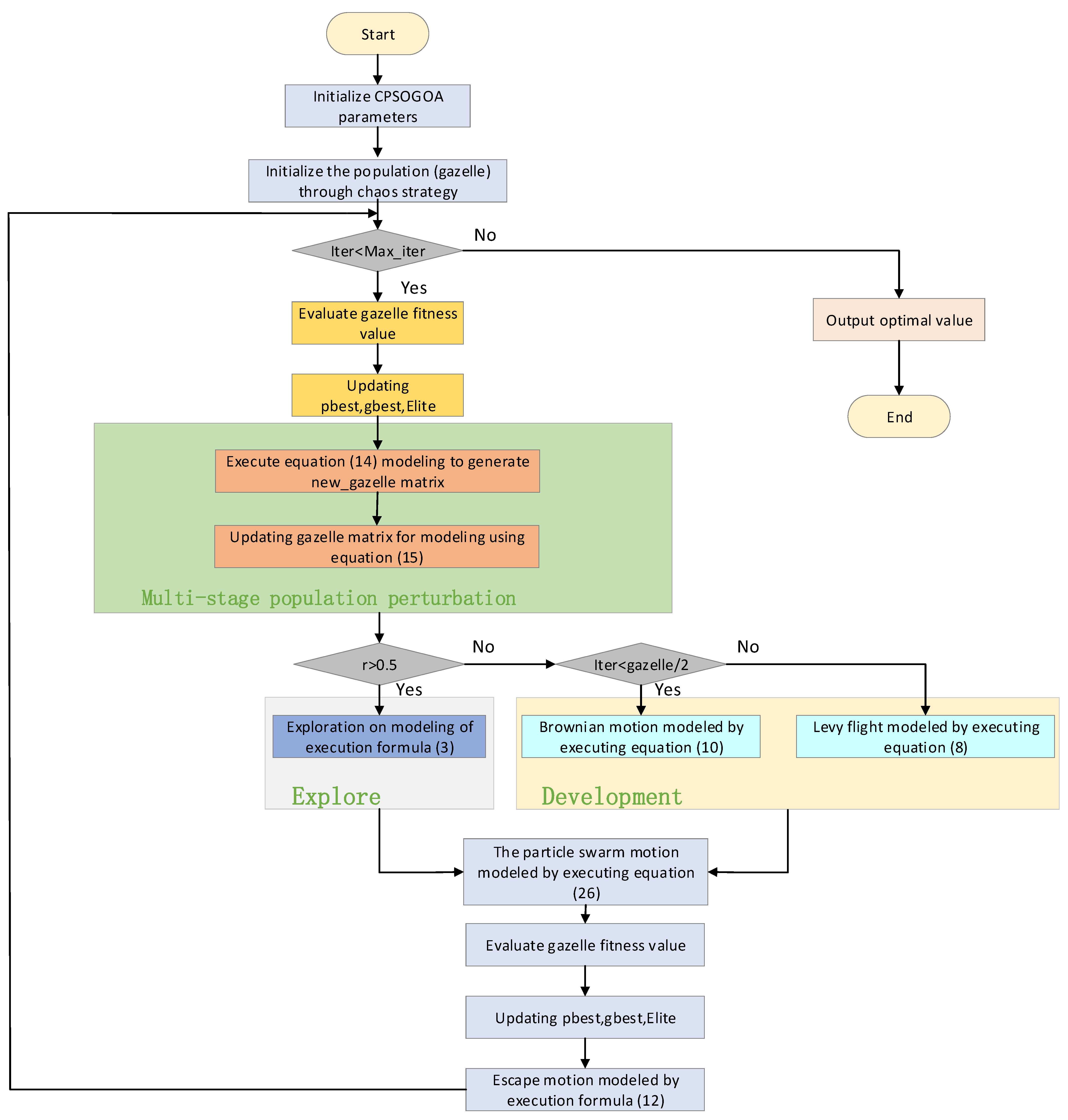
The pseudocode of the MPSOGOA outlines the process of the search optimization scheme as shown in Algorithm 1. The chaotic strategy improves the quality of the initial solutions, while the population-wide perturbation enhances the convergence speed and accuracy of the algorithm. Integration with PSO amplifies the role of individual experiences during the optimization process, preventing premature convergence of the algorithm. After meeting the termination conditions, the algorithm outputs the identified optimal solution. The combined action of the three strategies ensures both a high level of precision and an improved convergence speed of the optimization results, thereby guaranteeing that MPSOGOA can always find the optimal solution.
| Algorithm 1 Pseudocode of MPSOGOA |
| Initialize algorithm parameters s, μ, S, PSRs, C1, C2. |
| Use Piecewise mapping to initialize the population. |
| While (iter < max_iter) |
| Evaluate the fitness value of the gazelle. Construct pbest, gbest, and Elite. |
| For each gazelle in the population: |
| Generate a new gazelle matrix based on Equation (14). |
| Update the gazelle matrix according to Equation (15). |
| End For |
| For each gazelle in the population: |
| For each dimension: |
| If (mod (iter, 2) = 0) then |
| μ = −1 |
| Else |
| μ = 1 |
| End If |
| If (r > 0.5) then |
| Execute exploration activities on the gazelle matrix according to Equation (3). |
| Else |
| If iter < size(gazelle,1)/2 then |
| Perform Brownian motion on the gazelle matrix according to Equation (10). |
| Else |
| Execute Lévy flight on the gazelle matrix according to Equation (8). |
| End If |
| End If |
| End For |
| End For |
| Execute particle swarm movement on the gazelle matrix based on Equation (26). |
| Evaluate the fitness value of the gazelle. |
| Update pbest, gbest, and Elite. |
| Execute escape movement on the gazelle matrix according to Equation (12). |
| Iter = iter + 1 |
| End While |
| Return the optimal value from the population. |
According to the flowchart in Figure 2, the MPSOGOA process involves primarily initializing the population, evaluating the fitness of the gazelle, and updating candidate solutions. The complexity of MPSOGOA is determined by the maximum iteration count (iter_max), the population size (P), and the problem’s dimension (D). From the algorithm flowchart, it is evident that the algorithm complexity is composed of two parts, denoted as O(iter_max × D) + O(F). Among these, F represents the time consumed by the algorithm in evaluating various functions. Thus, the complete analysis of algorithm complexity is as follows: O(MPSOGOA) = O(iter_max × P × D) + O(CFE × P). The complexity analysis of MPSOGOA can be simplified to: O(MPSOGOA) = O(iter_max × P × D + CFE × P).
4. Experimental Design
This section presents an analysis of the simulation results of the MPSOGOA. The performance of the proposed MPSOGOA is evaluated using 35 test functions and 4 practical engineering design problems. The results of MPSOGOA in test functions and practical engineering applications are compared with the following algorithms: MPSOGOA, GOA, grey wolf optimizer (GWO) [51], sine cosine algorithm (SCA) [52], arithmetic optimization algorithm (AOA) [53], PSO [50], differential evolution (DE) [54], chimp optimization algorithm (Chimp) [55], biogeography-based optimization (BBO) [56], and golden jackal optimization (GJO) [57]. All experiments were conducted on a computer running on a 64-bit Windows 7 operating system equipped with a Core i5 CPU operating at a frequency of 2.50 GHz and 4.0 GB of RAM. The Matlab version used was R2021b. To minimize the impact of randomness on the algorithm, all algorithms were independently run 30 times for each test function, with the population size (P) set to 50 and the maximum iteration count (iter_max) set to 1000 generations. The parameter settings for all algorithms in the experiment are shown in Table 1.
To comprehensively evaluate the effectiveness of the algorithm, the following statistical evaluation indicators are utilized: best value, worst value, mean value, standard deviation (SD), and median value.
4.1. Test Function
Table 2 and Table 3 record the 35 test functions used to evaluate the performance of the MPSOGOA. The first 20 problems are classic test functions in optimization problems. Table 2 provides the test functions, their positions, and the corresponding optimal values. F1–F5 are continuous unimodal functions. F6 represents a discontinuous step function, while F7 denotes a quartic noise function. F8–F13 are multimodal functions, and F14–F20 are fixed-dimension multimodal functions. Table 3 presents 15 problems, including a selection of test functions from the CEC2014 and CEC2017 competitions. F21 and F22 are unimodal functions, F23–F31 and F35 are simple multimodal functions, and F34 represents a hybrid function. Unimodal functions typically have a single global optimum and are often used to test the exploratory capabilities of metaheuristic algorithms. Multimodal functions have multiple local optima, making them more complex than unimodal functions. Therefore, they are frequently employed to test whether optimization techniques possess good exploratory capabilities. The number of multimodal functions exponentially increases with the design variables, balancing exploration and exploitation to enhance the algorithm’s search efficiency and prevent it from getting trapped in local optima. These test functions are used to infer the potential for the algorithm to find optimal solutions in real-world problems.
4.2. Practical Engineering Applications
By testing the performance of optimization techniques on real-world engineering problems and designing corresponding parameter values, the overall design cost is minimized. This study focuses on the welding beam design problem, compression spring design problem, and pressure vessel design problem in mechanical engineering. Most engineering design problems in practical applications are governed by equality and inequality constraints, which are managed in the design objective function using penalty functions. The application of MPSOGOA to mechanical engineering design problems is compared with results obtained from nine other metaheuristic algorithms.
4.2.1. Welded Beam
Welded beam design is a problem of minimizing optimization, often utilized to assess the capability of optimization techniques in addressing practical issues. The welded beam design involves the manufacturing of a welded beam with the minimum cost under multiple constraints. The proposed MPSOGOA, along with 10 other metaheuristic algorithms, is applied to the welded beam design problem to minimize the cost of manufacturing the welded beam. Figure 3 provides an illustration of the welded beam. The decision variables that constrain the minimization of the cost of the welded beam design include the length (l), height (h), thickness (b), and weld thickness (h) of the steel bars. The constraints for the welded beam design encompass shear force (τ), bending stress (θ), column buckling load (Pc), beam deflection (δ), and lateral constraints, represented by WBD constraints. The objective function and penalty function for this problem is as follows:
The bounds of the variables are as follows:
The constraints are as follows:
The intermediate variables of the constraints are as follows:
where σmax = 3 × 10⁴ psi, P = 6 × 10³ lb, L = 14 in, δmax = 0.25 in, E = 30 × 106 psi, τmax = 13600 psi, and G = 1.2 × 10⁷ psi.
4.2.2. Compression Spring Design Issues
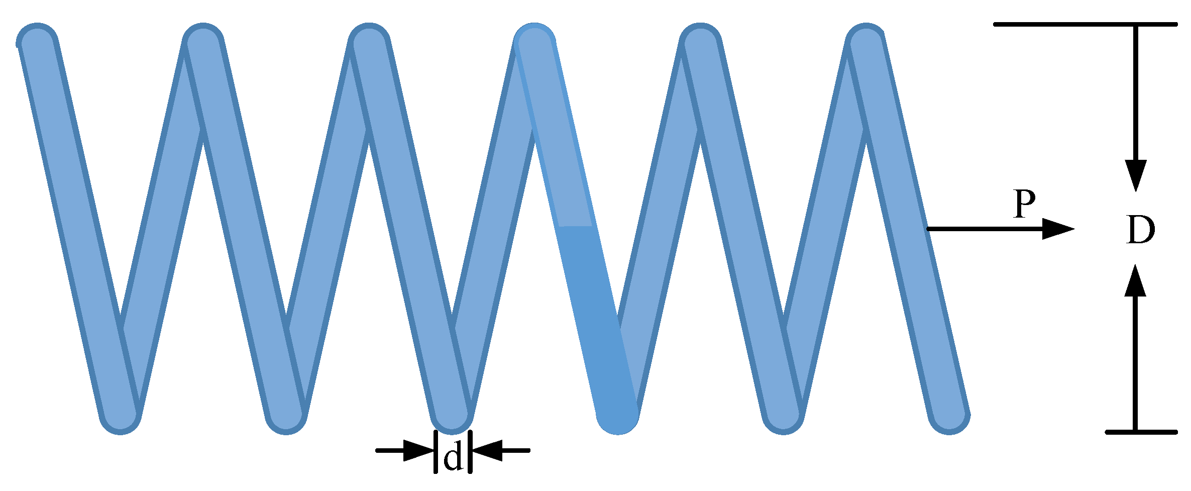
The objective of spring design is to minimize the total weight of the tension/compression spring. As depicted in Figure 4, this spring design problem is controlled by three parameters: the wire diameter (d), mean coil diameter (D), and number of active coils in the spring (P). The design function and constraint function for the spring design problem are given in Equations (24) and (25),
The boundary conditions of the variables are as follows:
The constraints of the spring design problem are as follows:
4.2.3. Pressure Vessel Design
The primary objective of the pressure vessel design problem is to minimize the production cost of the pressure vessel to the greatest extent possible (Figure 5). This problem is governed by four control parameters: the thickness of the pressure vessel (Ts), thickness of the head (Th), internal radius of the vessel (R), and length of the vessel head (L). The design function and constraint function for the pressure vessel design problem are provided in Equations (29) and (30), respectively,
The variation range of variables is as follows:
The constraints of the pressure vessel design problem are as follows:
5. Results and Discussion
In this section, to validate the performance of the proposed MPSOGOA, 35 test functions and 3 real-world engineering optimization problems are employed for performance testing, and comparisons are made with the original GOA and currently popular metaheuristic algorithms. The entire experiment is conducted in the following parts: (1) analysis of the experimental results of classical test functions, (2) analysis of the experimental results of the CEC2014 and CEC2017 composite test functions, (3) convergence performance of the MPSOGOA, and (4) result analysis of the 3 engineering optimization problems.
The performance of each algorithm is measured using five performance indicators: best value, worst value, average value, standard deviation, and median. Furthermore, the performance of the MPSOGOA is evaluated using Friedman rank sum test and Wilcoxon signed-rank test.
5.1. Test Function Results
5.1.1. Analysis of CEC2005 Experimental Results
Table 4 presents the experimental results of 10 algorithms on 20 benchmark functions, including the best results obtained from 30 independent runs (Best), the worst results (Worst), the mean values (Mean), the standard deviations (Std), the medians (Median), and the Wilcoxon signed-rank test rankings (Rank) of each algorithm across the 20 benchmark functions. The final ranking is determined by the Friedman rank sum ranking of each algorithm across the 20 benchmark functions.
Unimodal functions have only one optimal value, so they are often used to test the exploitation capability of algorithms. It can be seen from Table 4 that MPSOGOA shows the best performance on F1–F4. When solving F1, the convergence accuracy is improved by 180 orders of magnitude compared with GOA and 61 orders of magnitude compared with other algorithms. The convergence accuracy is also improved in different degrees. When solving F2, F3, and F4, the convergence accuracy is improved by more than 57 orders of magnitude and the standard deviation is improved by more than 40 orders of magnitude compared with GOA. Compared with GOA on F5–F7, the optimum values are improved. There is an improvement of two orders of magnitude on F6 and one order of magnitude on F7, with a smaller standard deviation. This means that the stability is also improved while the accuracy of convergence is improved. The above results indicate that MPSOGOA has good exploitation capability. F8–F20 is a multimodal function and a fixed-dimensional multimodal function, which usually has multiple extreme values and is often used to test the exploration ability of the algorithm. In the test of multimodal functions F8–F13, MPSOGOA performs better than other comparison algorithms on most functions and can find the optimal solution. When solving F12 and F13, the convergence accuracy of MPSOGOA is improved by two orders of magnitude compared with GOA. MPSOGOA shows excellent exploration ability on multimodal functions. In the test of F14 and F15, the optimal value of MPSOGOA is similar to other algorithms, but its standard deviation is lower. The experimental results show that MPSOGOA has good performance in solving unimodal and multimodal functions and excellent performance in convergence accuracy and stability.
Table 5 shows the Friedman rankings of the 10 algorithms in the benchmark test function. MPSOGOA achieved good results in the Friedman test. The MPSOGOA proposed in this article ranks first among the 10 optimization algorithms.
Furthermore, we conducted the Wilcoxon signed-rank test to assess the significance of differences between MPSOGOA and the other nine algorithms. When the p-value is less than 0.05, it is considered that there is a significant difference between the two algorithms for that specific function. The results of the Wilcoxon signed-rank test between MPSOGOA and the nine contrastive algorithms are presented in Table 6. It is evident from the table that MPSOGOA exhibits significant differences from the nine contrastive algorithms across the majority of the functions. Overall, across the 20 benchmark test functions, the performance of the MPSOGOA surpasses that of the nine contrastive algorithms, demonstrating strong competitiveness in the achieved results.
5.1.2. Analysis of Experimental Results of CEC2014 and CEC2017 Combined Test Functions
The ability of the algorithm to find the global optimal solution is evaluated by the combined test functions in CEC2014 and CEC2017. The test results of MPSOGOA and the other nine comparison algorithms are shown in Table 7. As can be seen from Table 7, the improvement of MPSOGOA has achieved better optimization effects in all combined functions. In the test of function F21, MPSOGOA becomes the only one that converges to the global optimal solution successfully. In addition, in the tests of F23, F24, and F31, the MPSOGOA and GOAs successfully find the global optimal solution. However, by comparing the standard deviation, it can be found that MPSOGOA has higher stability in the search process and can find the global optimal solution more stably. For F22, F25, F26, F27, F29, F30, F34, and F35 functions, MPSOGOA has achieved significant improvement in both optimization accuracy and stability compared with GOA. This series of improvements not only enhances the robustness of the algorithm, but also further validates the advantages of MPSOGOA in solving complex optimization problems. In summary, MPSOGOA successfully improves the ability of global optimal solution search by combining the advantages of PSO and gazelle optimization. Whether faced with the challenge of a single function or a series of combined functions, MPSOGOA has demonstrated its superior optimization performance and stability.
Compared to the GOA, MPSOGOA exhibits improved convergence accuracy and a strong ability to escape local optima. Additionally, it achieves smaller standard deviations, notably reducing the standard deviations in F21, F22, F24, and F31, suggesting that MPSOGOA significantly surpasses the GOA in terms of stability.
Table 8 shows the results of the Wilcoxon signed-rank test for 15 composite functions. The results show that there are significant differences between MPSOGOA and other algorithms on most test functions.
The rankings of the Friedman test are given in Table 9. MPSOGOA first among the 10 algorithms, proving that MPSOGOA’s optimization ability exceeds other algorithms. This shows that MPSOGOA has good optimization capabilities and can solve most optimization problems.
5.1.3. Convergence Speed
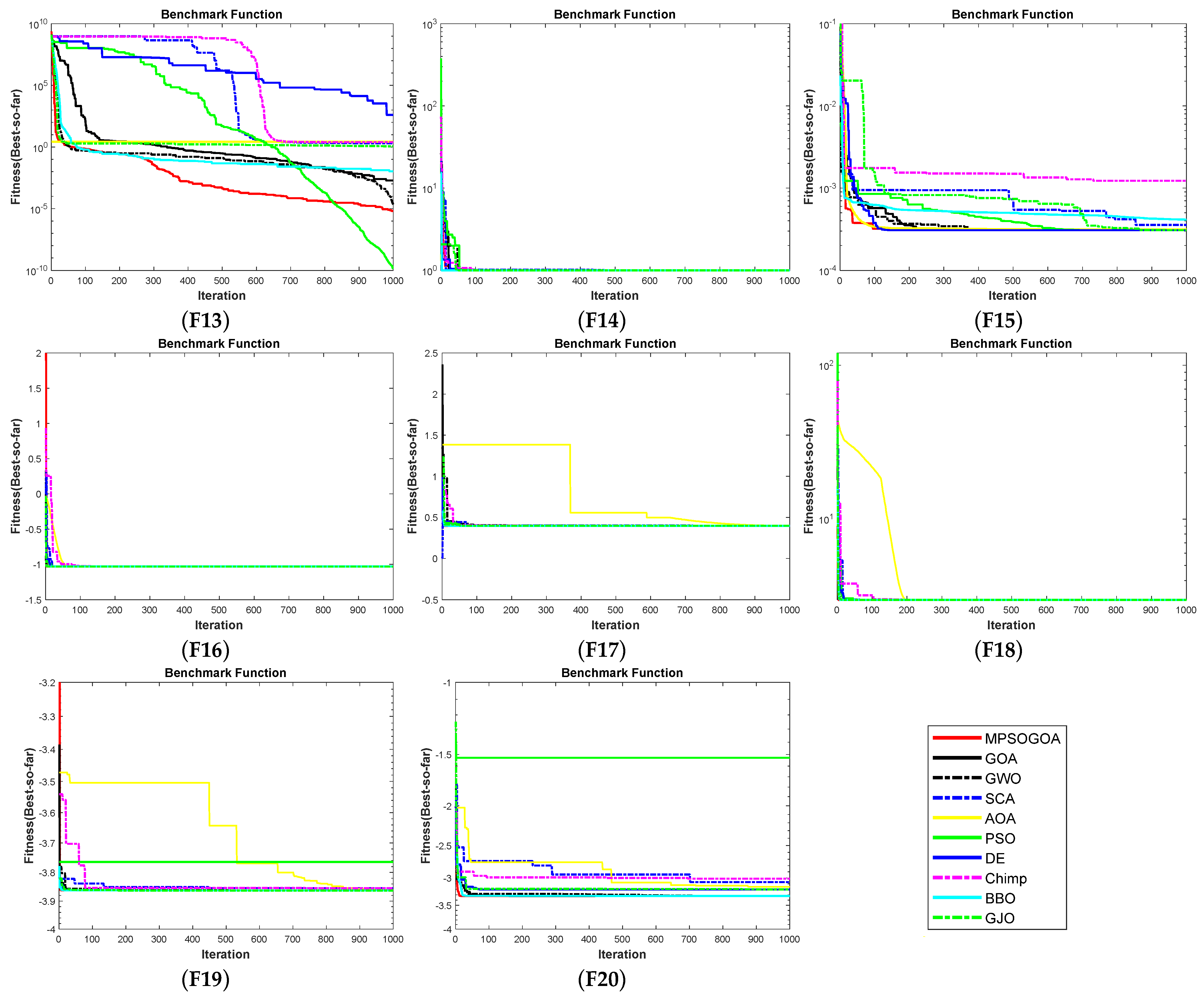
Figure 6 compares the convergence curves of MPSOGOA with the original GOA and eight other optimization algorithms on the classical test functions. The behavior of optimization algorithms that converge to the optimal solution early in the optimization process can lead to the inability of the algorithm to find the final global optimal solution. It can be observed that MPSOGOA quickly converges to the optimal solution in most test functions without being constrained by local optima. The convergence curves of F1–F4 demonstrate the accelerated convergence speed of MPSOGOA. The early convergence to the optimal solution in F5, F9, F10, F11, F15, and F20 is attributed to the role of the chaotic strategy and population-wide perturbation in the initial iterations. The algorithm stalls in the later iterations of F7, and the individual experience of particles and population-wide perturbation play a role in the later iterations, enabling the algorithm to escape local optima and eventually find the global optimal solution. Compared to GOA, MPSOGOA significantly converges faster to the global optimal solution in F1–F7, F9–F13, and F15.
Figure 7 shows the comparison of convergence curves of MPSOGOA, GOA, and eight other optimization algorithms in CEC2014 and CEC2017 combined test functions. Compared with other algorithms, MPSOGOA has an advantage in convergence speed. The convergence curve of MPSOGOA is always lower than the convergence curve of other algorithms, and the convergence curve drops significantly faster. The convergence rate of MPSOGOA on F21, F26, F27, F28, and F31 is obviously better than other algorithms. In the early stage of iteration, MPSOGOA’s convergence ability is far superior to other algorithms, and it can quickly approach the optimal solution in a short time. This is because the algorithm adopts PLCM for population initialization in the initial stage, constructs the initial population with relatively uniform distribution, and improves the quality of the initial population, especially in the initial stage of functions F21 and F31, which have better fitness values than other algorithms. In addition, MPSOGOA shows stable and fast convergence on function F23 with small fluctuation due to the combination of population global perturbation strategy and particle swarm strategy. This further confirms MPSOGOA’s significant advantages in terms of global convergence speed and optimization accuracy.
After comprehensive analysis of MPSOGOA’s optimization accuracy and convergence speed, the MPSOGOA has significantly improved both in terms of convergence speed and global optimization accuracy, and shows advantages in terms of stability. Compared with other algorithms, MPSOGOA has less fluctuation in results during multiple runs, meaning that its output results are more reliable and stable. The improved method is effective.
5.1.4. Ablation Experiment
Ablation experiments were conducted on MPSOGOA and GOA in order to comprehensively validate the effectiveness of the three proposed strategies during the optimization process. Three strategies were employed in this study to enhance the performance of GOA, leading to the following scenarios: the use of only the PWLC mapping strategy in the gazelle optimization algorithm (GOA1), the use of only population-wide disturbance in the gazelle optimization algorithm (GOA2), the use of only the PSO algorithm-integrated gazelle optimization algorithm (GOA3), the simultaneous use of PWLC mapping and population-wide disturbance strategies in the gazelle optimization algorithm (GOA4), the simultaneous use of PWLC mapping and PSO strategy-integrated gazelle optimization algorithm (GOA5), and the simultaneous use of population-wide disturbance and PSO strategy-integrated gazelle optimization algorithm (GOA6). The tests were based on classical test functions from Table 10 with a population size set at 50 and iteration count at 1000 in the experiments. Each algorithm was independently run 30 times, and calculations were performed for the optimal value, worst value, average value, standard deviation, and median.
It is evident that the convergence accuracy of the GOA1 algorithm from Table 10 and Figure 8, which incorporates only the PWLC mapping strategy, the GOA2 algorithm with only the population-wide disturbance strategy, and the GOA3 algorithm with only the strategy integrated with PSO, surpasses that of the standard GOA across 15 test functions. Furthermore, the convergence speed on these 15 test functions is also superior to that of the GOA. This indicates the efficacy of each strategy in enhancing the GOA. A comparative analysis between the optimization results of GOA1, GOA2, and GOA3 with GOA4, GOA5, and GOA6 reveals that the convergence accuracy achieved by the fusion of two improvement strategies is generally superior to that achieved using a single improvement strategy.
Simultaneously, the convergence speed is also enhanced, underscoring the synergistic and stable effectiveness of all improvement strategies. Their collective impact serves to improve the solving capability of MSPGOA. It can be also observed that the convergence accuracy of MPSOGOA from Table 10 and Figure 8, which integrate three improvement strategies, surpasses that of GOAs employing one or two improvement strategies. Notably, MPSOGOA exhibits the fastest convergence speed among the 15 test functions.
5.2. Engineering Problem Results
5.2.1. Welded Beam
Table 11 presents the experimental results of the welded beam design problem. The table includes the optimal solution obtained by MPSOGOA and the other nine optimization algorithms (GOA, GWO, SCA, AOA, PSO, DE, Chimp, BBO, and GJO) in the welded beam design problem, along with their corresponding optimal variables, worst value, mean, standard deviation, and median, as well as the values from the signed-rank test. It is evident from the table that the statistical results of all performance aspects of the proposed MPSOGOA in the welded beam design problem are optimal, indicating its strong optimization effectiveness in solving practical engineering applications and effectively reducing the cost of the welded beam design problem. The table indicates that MPSOGOA achieves the optimal cost value of 1.67022 for the welded beam design, with the corresponding optimal decision variables being steel bar length 0.198832, steel bar height 3.33737, steel bar thickness 9.19202, and weld thickness 0.198832. Compared to the original GOA, MPSOGOA exhibits a smaller standard deviation, signifying its superior stability. The results of the signed-rank test in the table indicate that the p-values for MPSOGOA and the other nine algorithms are all less than 0.05, indicating no statistical significance.
Figure 9 shows the convergence curves of each algorithm on the welded beam design problem. These algorithms can quickly converge to the optimal solution.
5.2.2. Compression Spring Design
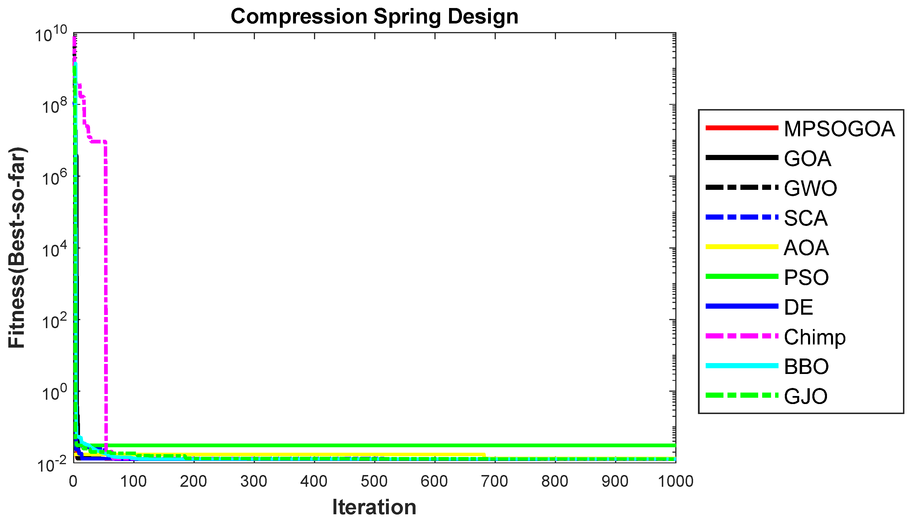
Table 12 presents the experimental results for the compression spring design problem. The table includes the optimal solution obtained by MPSOGOA and the other nine optimization algorithms in the compression spring design problem, along with their corresponding optimal variables, worst value, mean, standard deviation, and median, as well as the values from the signed-rank test. It is evident from the table that MPSOGOA achieves the optimal cost value of 0.0126652 for the compression spring design, with the corresponding optimal decision variables being wire diameter 0.0516905, mean coil diameter 0.356752, and the number of effective coils in the spring 11.287. MPSOGOA and DE achieve the same optimal cost value in the compression spring design problem. Furthermore, when compared to the original GOA, MPSOGOA outperforms GOA in all statistical data aspects. The results of the signed-rank test in the table indicate that the p-values for MPSOGOA and the other nine algorithms are all less than 0.05, indicating no statistical significance.
Figure 10 shows the convergence curves of each algorithm on the welded beam design problem. Except for the PSO and Chimp algorithms, other algorithms can quickly converge to the optimal solution.
5.2.3. Pressure Vessel Design
Table 13 presents the experimental results for the pressure vessel design problem. The table includes the optimal solution obtained by MPSOGOA and the other nine optimization algorithms in the pressure vessel design problem, along with their corresponding optimal variables, worst value, mean, standard deviation, and median, as well as the values from the signed-rank test. It is evident from the table that the statistical results of all performance aspects of the proposed MPSOGOA in the pressure vessel design problem are optimal, indicating its strong optimization effectiveness in solving practical engineering applications and effectively reducing the cost of the pressure vessel design problem. From the table, it can be seen that MPSOGOA achieves the optimal cost value of 5885.33 for the pressure vessel design, with the corresponding optimal decision variables being pressure vessel thickness 0.778168, head thickness 0.384649, internal vessel radius 40.3196, and vessel head length 200. Compared to the original GOA, MPSOGOA exhibits significant improvement in terms of standard deviation, suggesting its superior stability in the process of seeking the optimal solution. The results of the signed-rank test in the table indicate that the p-values for MPSOGOA and the other nine algorithms are all less than 0.05, indicating no statistical significance.
Figure 11 shows the convergence curves of each algorithm on the pressure vessel design problem. MPSOGOA, GOA, GWO, SCA, DE, Chimp, and GJO are all able to quickly converge to the optimal solution. AOA falls into a local optimum and eventually escapes from the local optimum, and optimally converges to the optimal value.
6. Conclusions
In this paper, we present an enhanced version of the MPSOGOA, incorporating a chaotic strategy to refine the quality of the initial population. A population-wide perturbation is strategically applied to augment the convergence speed and precision of the algorithm. Furthermore, through synergistic integration with PSO, emphasis is placed on leveraging individual experiences within the optimization process, culminating in a comprehensive enhancement of algorithmic performance. MPSOGOA demonstrates promising outcomes across a suite of 35 test functions and 4 engineering design challenges. Notably, in a majority of the test functions, MPSOGOA consistently identifies optimal solutions, displaying diminished standard deviations compared to the original GOA. This signifies a marked improvement in stability when contrasted with GOA. Additionally, in the Friedman test, MPSOGOA attains the foremost position among all comparative algorithms. Across the spectrum of four engineering design problems, the performance metrics of MPSOGOA surpass those of esteemed optimization algorithms including GOA, GWO, SCA, AOA, PSO, DE, Chimp, BBO, and GJO. To summarize, based on the comparative analysis of algorithms in both test functions and engineering designs, MPSOGOA emerges as a superior choice for addressing optimization challenges.
Author Contributions
Conceptualization, S.Q., H.Z., W.S. and J.Y.; methodology, J.Y. and J.W.; validation, S.Q., H.Z. and J.W.; formal analysis, J.Y.; investigation, J.Y.; resources, J.W.; data curation, H.Z.; writing—original draft preparation, S.Q. and H.Z.; writing—review and editing, J.Y. and J.W.; supervision, H.Z. All authors have read and agreed to the published version of the manuscript.
Funding
This research received no external funding.
Data Availability Statement
Data are contained within the article.
Conflicts of Interest
The authors declare no conflicts of interest.
References
- Aditya, N.; Mahapatra, S.S. Switching from exploration to exploitation in gravitational search algorithm based on diversity with Chaos. Inf. Sci. 2023, 635, 298–327. [Google Scholar] [CrossRef]
- Gonzalez-Ayala, P.; Alejo-Reyes, A.; Cuevas, E.; Mendoza, A. A Modified Simulated Annealing (MSA) Algorithm to Solve the Supplier Selection and Order Quantity Allocation Problem with Non-Linear Freight Rates. Axioms 2023, 12, 459. [Google Scholar] [CrossRef]
- Zheng, W.M.; Liu, N.; Chai, Q.W.; Liu, Y. Application of improved black hole algorithm in prolonging the lifetime of wireless sensor network. Complex Intell. Syst. 2023, 9, 5817–5829. [Google Scholar] [CrossRef]
- Mansuwan, K.; Jirapong, P.; Thararak, P. Optimal battery energy storage planning and control strategy for grid modernization using improved genetic algorithm. Energy Rep. 2023, 9, 236–241. [Google Scholar] [CrossRef]
- Wei, L.; Zhang, Q.; Yang, B. Improved Biogeography-Based Optimization Algorithm Based on Hybrid Migration and Dual-Mode Mutation Strategy. Fractal Fract. 2022, 6, 597. [Google Scholar] [CrossRef]
- Şahman, M.A.; Korkmaz, S. Discrete artificial algae algorithm for solving job-shop scheduling problems. Knowl.-Based Syst. 2022, 256, 109711. [Google Scholar] [CrossRef]
- Salimon, S.A.; Adebayo, I.G.; Adepoju, G.A.; Adewuyi, O.B. Optimal Allocation of Distribution Static Synchronous Compensators in Distribution Networks Considering Various Load Models Using the Black Widow Optimization Algorithm. Sustainability 2023, 15, 15623. [Google Scholar] [CrossRef]
- Umam, M.S.; Mustafid, M.; Suryono, S. A hybrid genetic algorithm and tabu search for minimizing makespan in flow shop scheduling problem. J. King Saud Univ. -Comput. Inf. Sci. 2022, 34, 7459–7467. [Google Scholar] [CrossRef]
- János, M.M.; Artúr, S.; Gyula, G. Environmental and economic multi-objective optimization of a household level hybrid renewable energy system by genetic algorithm. Appl. Energy 2020, 269, 115058. [Google Scholar]
- Lodewijks, G.; Cao, Y.; Zhao, N.; Zhang, H. Reducing CO2 emissions of an airport baggage handling transport system using a particle swarm optimization algorithm. IEEE Access 2021, 9, 121894–121905. [Google Scholar] [CrossRef]
- Abualigah, L.; Alkhrabsheh, M. Amended hybrid multi-verse optimizer with genetic algorithm for solving task scheduling problem in cloud computing. J. Supercomput. 2021, 78, 740–765. [Google Scholar] [CrossRef]
- Hussain, B.; Khan, A.; Javaid, N.; Hasan, Q.U.; AMalik, S.; Ahmad, O.; Dar, A.H.; Kazmi, A. A WeightedSum PSO Algorithm for HEMS A New Approach for the Design and Diversified Performance Analysis. Electronics 2019, 8, 180. [Google Scholar] [CrossRef]
- Paul, K.; Hati, D. A novel hybrid Harris hawk optimization and sine cosine algorithm based home energy management system for residential buildings. Build. Serv. Eng. Res. Technol. 2023, 44, 459–480. [Google Scholar] [CrossRef]
- Jiang, C.; Yang, S.; Nie, P.; Xiang, X. Multi-objective structural profile optimization of ships based on improved Artificial Bee Colony Algorithm and structural component library. Ocean. Eng. 2023, 283, 115124. [Google Scholar] [CrossRef]
- Abd Elaziz, M.; Dahou, A.; Mabrouk, A.; El-Sappagh, S.; Aseeri, A.O. An efficient artificial rabbits optimization based on mutation strategy for skin cancer prediction. Comput. Biol. Med. 2023, 163, 107154. [Google Scholar] [CrossRef] [PubMed]
- Bishla, S.; Khosla, A. Enhanced chimp optimized self-tuned FOPR controller for battery scheduling using Grid and Solar PV Sources. J. Energy Storage 2023, 66, 107403. [Google Scholar] [CrossRef]
- Percin, H.B.; Caliskan, A. Whale optimization algorithm based MPPT control of a fuel cell system. Int. J. Hydrogen Energy 2023, 48, 23230–23241. [Google Scholar] [CrossRef]
- Jagadish Kumar, N.; Balasubramanian, C. Cost-efficient resource scheduling in cloud for big data processing using metaheuristic search black widow optimization (MS-BWO) algorithm. J. Intell. Fuzzy Syst. 2023, 44, 4397–4417. [Google Scholar] [CrossRef]
- Zeng, C.; Qin, T.; Tan, W.; Lin, C.; Zhu, Z.; Yang, J.; Yuan, S. Coverage Optimization of Heterogeneous Wireless Sensor Network Based on Improved Wild Horse Optimizer. Biomimetics 2023, 8, 70. [Google Scholar] [CrossRef]
- Chhabra, A.; Hussien, A.G.; Hashim, F.A. Improved bald eagle search algorithm for global optimization and feature selection. Alex. Eng. J. 2023, 68, 141–180. [Google Scholar] [CrossRef]
- Liu, Y.; Sun, J.; Shang, Y.; Zhang, X.; Ren, S.; Wang, D. A novel remaining useful life prediction method for lithium-ion battery based on long short-term memory network optimized by improved sparrow search algorithm. J. Energy Storage 2023, 61, 106645. [Google Scholar] [CrossRef]
- Xu, M.; Song, Q.; Xi, M.; Zhou, Z. Binary arithmetic optimization algorithm for feature selection. Soft Comput. 2023, 27, 11395–11429. [Google Scholar] [CrossRef] [PubMed]
- Chen, M.; Huo, J.; Duan, Y. A hybrid biogeography-based optimization algorithm for three-dimensional bin size designing and packing problem. Comput. Ind. Eng. 2023, 180, 109239. [Google Scholar] [CrossRef]
- Long, Y.; Liu, S.; Qiu, D.; Li, C.; Guo, X.; Shi, B.; AbouOmar, M.S. Local Path Planning with Multiple Constraints for USV Based on Improved Bacterial Foraging Optimization Algorithm. J. Mar. Sci. Eng. 2023, 11, 489. [Google Scholar] [CrossRef]
- Zou, D.; Li, M.; Ouyang, H. A MOEA/D approach using two crossover strategies for the optimal dispatches of the combined cooling, heating, and power systems. Appl. Energy 2023, 347, 121498. [Google Scholar] [CrossRef]
- Ramachandran, M.; Mirjalili, S.; Nazari-Heris, M.; Parvathysankar, D.S.; Sundaram, A.; Gnanakkan, C.A.R.C. A hybrid grasshopper optimization algorithm and harris hawks optimizer for combined heat and power economic dispatch problem. Eng. Appl. Artif. Intell. 2022, 111, 104753. [Google Scholar] [CrossRef]
- Hamza, M.A.; Alshahrani, H.M.; Dhahbi, S.; Nour, M.K.; Al Duhayyim, M.; El Din, E.M.; Yaseen, I.; Motwakel, A. Differential Evolution with Arithmetic Optimization Algorithm Enabled Multi-Hop Routing Protocol. Comput. Syst. Sci. Eng. 2023, 45, 1759–1773. [Google Scholar] [CrossRef]
- Pashaei, E.; Pashaei, E. Hybrid binary arithmetic optimization algorithm with simulated annealing for feature selection in high-dimensional biomedical data. J. Supercomput. 2022, 78, 15598–15637. [Google Scholar] [CrossRef]
- Bhowmik, S.; Acharyya, S. Image encryption approach using improved chaotic system incorporated with differential evolution and genetic algorithm. J. Inf. Secur. Appl. 2023, 72, 103391. [Google Scholar] [CrossRef]
- Panahizadeh, V.; Hamidi, E.; Daneshpayeh, S.; Saeifar, H. Optimization of impact strength and elastic modulus of polyamide-based nanocomposites: Using particle swarm optimization method. J. Elastomers Plast. 2024, 56, 244–261. [Google Scholar] [CrossRef]
- Kim, K.H.; Jung, Y.H.; Shin, Y.J.; Shin, J.H. Optimizing the drainage system of subsea tunnels using the PSO algorithm. Mar. Georesources Geotechnol. 2024, 42, 266–278. [Google Scholar] [CrossRef]
- Pal, K.; Verma, K.; Gandotra, R. Optimal location of FACTS devices with EVCS in power system network using PSO. e-Prime—Adv. Electr. Eng. Electron. Energy 2024, 7, 100482. [Google Scholar] [CrossRef]
- Kang, Z.; Duan, R.; Zheng, Z.; Xiao, X.; Shen, C.; Hu, C.; Tang, S.; Qin, W. Grid aided combined heat and power generation system for rural village in north China plain using improved PSO algorithm. J. Clean. Prod. 2024, 435, 140461. [Google Scholar] [CrossRef]
- Sirisumrannukul, S.; Intaraumnauy, T.; Piamvilai, N. Optimal control of cooling management system for energy conservation in smart home with ANNs-PSO data analytics microservice platform. Heliyon 2024, 10, e26937. [Google Scholar] [CrossRef] [PubMed]
- Sathasivam, K.; Garip, I.; Saeed, S.H.; Yais, Y.; Alanssari, A.I.; Hussein, A.A.; Hammoode, J.A.; Lafta, A.M. A Novel MPPT Method Based on PSO and ABC Algorithms for Solar Cell. Electr. Power Compon. Syst. 2024, 52, 653–664. [Google Scholar] [CrossRef]
- Hadi, N.; Jalal, B. Investigation of river water pollution using Muskingum method and particle swarm optimization (PSO) algorithm. Appl. Water Sci. 2024, 14, 68. [Google Scholar]
- Shaikh, M.S.; Raj, S.; Babu, R.; Kumar, S.; Sagrolikar, K. A hybrid moth–flame algorithm with particle swarm optimization with application in power transmission and distribution. Decis. Anal. J. 2023, 6, 100182. [Google Scholar] [CrossRef]
- Makhija, D.; Sudhakar, C.; Reddy, P.B.; Kumari, V. Workflow Scheduling in Cloud Computing Environment by Combining Particle Swarm Optimization and Grey Wolf Optimization. Comput. Sci. Eng. Int. J. 2022, 12, 1–10. [Google Scholar] [CrossRef]
- Adekilekun, M.T.; Abiola, G.A.; Olajide, M.O. Hybrid Optimization Technique for Solving Combined Economic Emission Dispatch Problem of Power Systems. Turk. J. Electr. Power Energy Syst. 2022, 2, 158–167. [Google Scholar]
- Osei-Kwakye, J.; Han, F.; Amponsah, A.A.; Ling, Q.; Abeo, T.A. A hybrid optimization method by incorporating adaptive response strategy for Feedforward neural network. Connect. Sci. 2022, 34, 578–607. [Google Scholar] [CrossRef]
- Wang, N.; Wang, J.S.; Zhu, L.F.; Wang, H.Y.; Wang, G. A novel dynamic clustering method by integrating marine predators algorithm and particle swarm optimization algorithm. IEEE Access 2020, 9, 3557–3569. [Google Scholar] [CrossRef]
- Samantaray, S.; Sahoo, P.; Sahoo, A.; Satapathy, D.P. Flood discharge prediction using improved ANFIS model combined with hybrid particle swarm optimisation and slime mould algorithm. Environ. Sci. Pollut. Res. 2023, 30, 83845–83872. [Google Scholar] [CrossRef]
- Wang, D.; Liu, L.; Ben, Y.; Dai, P.; Wang, J. Seabed Terrain-Aided Navigation Algorithm Based on Combining Artificial Bee Colony and Particle Swarm Optimization. Appl. Sci. 2023, 13, 1166. [Google Scholar] [CrossRef]
- Agushaka, J.O.; Ezugwu, A.E.; Abualigah, L. Gazelle optimization algorithm: A novel nature-inspired metaheuristic optimizer. Neural Comput. Appl. 2023, 35, 4099–4131. [Google Scholar] [CrossRef]
- Lu, W.; Shi, C.; Fu, H.; Xu, Y. A Power Transformer Fault Diagnosis Method Based on Improved Sand Cat Swarm Optimization Algorithm and Bidirectional Gated Recurrent Unit. Electronics 2023, 12, 672. [Google Scholar] [CrossRef]
- Nan, A.; Liyong, B. Particle Swarm Algorithm Based on Homogenized Logistic Mapping and Its Application in Antenna Parameter Optimization. Int. J. Inf. Commun. Sci. 2022, 7, 1–6. [Google Scholar]
- Yang, D.D.; Mei, M.; Zhu, Y.J.; He, X.; Xu, Y.; Wu, W. Coverage Optimization of WSNs Based on Enhanced Multi-Objective Salp Swarm Algorithm. Appl. Sci. 2023, 13, 11252. [Google Scholar] [CrossRef]
- Wei, X.; Zhang, Y.; Zhao, Y. Evacuation path planning based on the hybrid improved sparrow search optimization algorithm. Fire 2023, 6, 380. [Google Scholar] [CrossRef]
- Zheng, X.; Nie, B.; Chen, J.; Du, Y.; Zhang, Y.; Jin, H. An improved particle swarm optimization combined with double-chaos search. Math. Biosci. Eng. 2023, 20, 15737–15764. [Google Scholar] [CrossRef]
- Ozcan, E.; Mohan, C.K. Particle swarm optimization: Surfing the waves. In Proceedings of the 1999 Congress on Evolutionary Computation-CEC99 (Cat. No. 99TH8406), Washington, DC, USA, 6–9 July 1999; IEEE: Piscataway, NJ, USA, 1999; Volume 3, pp. 1939–1944. [Google Scholar]
- Mirjalili, S.; Mirjalili, S.M.; Lewis, A. Grey wolf optimizer. Adv. Eng. Softw. 2014, 69, 46–61. [Google Scholar] [CrossRef]
- Mirjalili, S. SCA: A sine cosine algorithm for solving optimization problems. Knowl. -Based Syst. 2016, 96, 120–133. [Google Scholar] [CrossRef]
- Abualigah, L.; Diabat, A.; Mirjalili, S.; Abd Elaziz, M.; Gandomi, A.H. The arithmetic optimization algorithm. Comput. Methods Appl. Mech. Eng. 2021, 376, 113609. [Google Scholar] [CrossRef]
- Storn, R.; Price, K. Differential evolution–a simple and efficient heuristic for global optimization over continuous spaces. J. Glob. Optim. 1997, 11, 341–359. [Google Scholar] [CrossRef]
- Khishe, M.; Mosavi, M.R. Chimp optimization algorithm. Expert Syst. Appl. 2020, 149, 113338. [Google Scholar] [CrossRef]
- Simon, D. Biogeography-based optimization. IEEE Trans. Evol. Comput. 2008, 12, 702–713. [Google Scholar] [CrossRef]
- Chopra, N.; Ansari, M.M. Golden jackal optimization: A novel nature-inspired optimizer for engineering applications. Expert Syst. Appl. 2022, 198, 116924. [Google Scholar] [CrossRef]
Figure 1.
Piecewise mapping distribution plot and histogram. (a) Piecewise mapping distribution histogram; (b) Piecewise mapping distribution scatter plot; (c) Logistic map distribution histogram; (d) Logistic mapping distribution scatter plot.
Figure 1.
Piecewise mapping distribution plot and histogram. (a) Piecewise mapping distribution histogram; (b) Piecewise mapping distribution scatter plot; (c) Logistic map distribution histogram; (d) Logistic mapping distribution scatter plot.


Figure 2.
MPSOGOA flow chart.

Figure 3.
Schematic diagram of welded beam design.

Figure 4.
Schematic diagram of compression spring design problem.

Figure 5.
Schematic diagram of pressure vessel design issues.

Figure 6.
CEC2005 test function convergence diagram.


Figure 7.
Convergence diagram of CEC2014 and CEC2017 group and test functions.

Figure 8.
Convergence results of ablation experiments based on CEC2005.


Figure 9.
Convergence curve of WBD.

Figure 10.
Convergence curve of CSD.

Figure 11.
Convergence curve of PVD.


Table 1.
Algorithm parameter settings for comparison.
| Algorithm | Parameter | Parameter Value |
|---|---|---|
| GOA | PSRs | 0.34 |
| S | 0.88 | |
| GWO | a | [0, 2] |
| r1f r2 | [0, 1] | |
| SCA | a | 2 |
| AOA | 5 | |
| 0.05 | ||
| PSO | C1, C2 | 2 |
| Wmax | 0.9 | |
| Wmin | 0.2 | |
| DE | Lower bound of scale factor | 0.2 |
| Upper bound of scale factor | 0.8 | |
| BBO | nKeep | 0.2 |
| Pmutation | 0.9 |
Table 2.
Classic test function.
| ID | Function | Dim | Range | Global |
|---|---|---|---|---|
| F1 | 30 | [−100, 100] | 0 | |
| F2 | 30 | [−10, 10] | 0 | |
| F3 | 30 | [−100, 100] | 0 | |
| F4 | 30 | [−100, 100] | 0 | |
| F5 | 30 | [−30, 30] | 0 | |
| F6 | 30 | [−100, 100] | 0 | |
| F7 | 30 | [−128, 128] | 0 | |
| F8 | 30 | [−500, 500] | 418.9829 Dim | |
| F9 | 30 | [−5.12, 5.12] | 0 | |
| F10 | 30 | [−32, 32] | 0 | |
| F11 | 30 | [−600, 600] | 0 | |
| F12 | 30 | [−50, 50] | 0 | |
| F13 | 30 | [−50, 50] | 0 | |
| F14 | 2 | [−65, 65] | 1 | |
| F15 | 4 | [−5, 5] | 0.00030 | |
| F16 | 2 | [−5, 5] | −1.0316 | |
| F17 | 2 | [−5, 5] | 0.398 | |
| F18 | 2 | [−2, 2] | 3 | |
| F19 | 3 | [1, 3] | −3.86 | |
| F20 | 6 | [0, 1] | −3.32 |
Table 3.
CEC2014 and CEC2017 combined test functions.
| ID | Function | Fi |
|---|---|---|
| F21 | Rotated High Conditioned Elliptic Function (CEC 2014 F1) | 100 |
| F22 | Shifted and Rotated Bent Cigar Function (CEC 2017 F1) | 100 |
| F23 | Shifted and Rotated Rosenbrock’s Function (CEC 2017 F3) | 300 |
| F24 | Shifted and Rotated Rastrigin’s Function (CEC 2017 F4) | 400 |
| F25 | Shifted and Rotated Expanded Scaffer’s F6 Function (CEC 2017 F5) | 500 |
| F26 | Shifted and Rotated Weierstrass Function (CEC 2014 F6) | 600 |
| F27 | Shifted and Rotated Lunacek Bi_ Rastrigin Function (CEC 2017 F6) | 600 |
| F28 | Shifted and Rotated Non-Continuous Rastrigin’sFunction (CEC 2017 F7) | 700 |
| F29 | Shifted Rastrigin’s Function (CEC 2014 F8) | 800 |
| F30 | Shifted and Rotated Levy Function (CEC 2017 F8) | 800 |
| F31 | Shifted and Rotated Schwefel’s Function (CEC 2017 F9) | 900 |
| F32 | Shifted Schwefel’s Function (CEC 2014 F10) | 1000 |
| F33 | Shifted and Rotated Schwefel’s Function (CEC 2014 F11) | 1100 |
| F34 | Hybrid Function 2 (n = 3) (CEC 2017 F11) | 1100 |
| F35 | Shifted and Rotated Expanded Scaffers F6 Function (CEC 2014 F16) | 1600 |
Table 4.
CEC2005 test results.
| Function | Value | MPSOGOA | GOA | GWO | SCA | AOA | PSO | DE | Chimp | BBO | GJO |
|---|---|---|---|---|---|---|---|---|---|---|---|
| F1 | Best | 2.7433 × 10−268 | 2.89154 × 10−88 | 8.50069 × 10−73 | 2.54974 × 10⁻⁸ | 1.0643 × 10−207 | 9.47085 × 10⁻¹² | 51.648 | 1.3579 × 10⁻²⁷ | 0.324489 | 1.2726 × 10−132 |
| Worst | 1.5559 × 10−214 | 3.40688 × 10⁻²⁴ | 1.00555 × 10−69 | 0.0243454 | 2.9067 × 10−95 | 9.19223 × 10⁻⁸ | 261.883 | 2.01606 × 10⁻¹⁸ | 1.18724 | 5.5191 × 10−127 | |
| Average | 5.1864 × 10−216 | 1.13563 × 10⁻²⁵ | 1.63935 × 10−70 | 0.0013788 | 2.59489 × 10−96 | 3.99524 × 10⁻⁹ | 131.843 | 2.11538 × 10⁻¹⁹ | 0.619129 | 5.5742 × 10−128 | |
| SD | 0 | 6.22009 × 10⁻²⁵ | 2.59621 × 10−70 | 0.00450527 | 7.96026 × 10−96 | 1.66386 × 10⁻⁸ | 49.421 | 5.13648 × 10⁻¹⁹ | 0.166653 | 1.3812 × 10−127 | |
| Median | 5.0964 × 10−252 | 5.30668 × 10−78 | 5.55451 × 10−71 | 8.70929 × 10⁻⁵ | 8.3471 × 10−131 | 6.60832 × 10⁻¹⁰ | 124.27 | 2.16579 × 10⁻²² | 0.579377 | 9.8842 × 10−130 | |
| F2 | Best | 1.5987 × 10−137 | 9.12414 × 10−57 | 9.04044 × 10−42 | 9.4068 × 10−09 | 0 | 6.63994 × 10⁻⁷ | 18.9427 | 8.76387 × 10⁻¹⁹ | 0.158091 | 6.77923 × 10−76 |
| Worst | 1.006 × 10−117 | 1.5473 × 10⁻²⁰ | 4.17611 × 10−40 | 6.56174 × 10⁻⁵ | 1.3602 × 10−129 | 177.155 | 55.6008 | 1.66733 × 10⁻¹² | 0.318038 | 6.08005 × 10−73 | |
| Average | 3.3535 × 10−119 | 5.58832 × 10⁻²² | 6.87572 × 10−41 | 4.5299 × 10⁻⁶ | 4.5341 × 10−131 | 5.90526 | 41.1955 | 1.32586 × 10⁻¹³ | 0.245152 | 6.65278 × 10−74 | |
| SD | 1.8366 × 10−118 | 2.82639 × 10⁻²¹ | 9.28251 × 10−41 | 1.25192 × 10⁻⁵ | 2.4834 × 10−130 | 32.3439 | 9.34487 | 3.44014 × 10⁻¹³ | 0.0386638 | 1.37309 × 10−73 | |
| Median | 6.7837 × 10−133 | 7.41398 × 10−49 | 3.6684 × 10−41 | 4.08327 × 10⁻⁷ | 5.8246 × 10−210 | 1.47627 × 10⁻⁵ | 42.7029 | 1.31203 × 10⁻¹⁴ | 0.251466 | 1.30119 × 10−74 | |
| F3 | Best | 4.35826 × 10−69 | 2.63083 × 10⁻¹² | 2.90856 × 10⁻²⁴ | 27.8478 | 0 | 236.094 | 22,892.9 | 6.69748 × 10⁻¹⁰ | 34.0053 | 2.07975 × 10−58 |
| Worst | 4.07582 × 10−43 | 0.00307754 | 3.26631 × 10⁻¹⁷ | 10,369.5 | 2.50525 × 10−45 | 2541.13 | 38,833.8 | 0.019964 | 147.677 | 1.01149 × 10−43 | |
| Average | 1.40494 × 10−44 | 0.00021169 | 2.07546 × 10⁻¹⁸ | 2522.16 | 8.35084 × 10−47 | 929.7 | 29,602.2 | 0.0010311 | 85.0581 | 3.37788 × 10−45 | |
| SD | 7.4369 × 10−44 | 0.00062157 | 7.24266 × 10⁻¹⁸ | 2409.21 | 4.57394 × 10−46 | 484.589 | 4207.89 | 0.00363366 | 31.1403 | 1.84661 × 10−44 | |
| Median | 7.55093 × 10−62 | 1.02692 × 10⁻⁷ | 1.63874 × 10⁻²¹ | 1486.21 | 2.2905 × 10−102 | 889.357 | 28,564 | 4.07225 × 10⁻⁵ | 77.9158 | 7.89966 × 10−50 | |
| F4 | Best | 1.9656 × 10−108 | 3.9303 × 10⁻²⁸ | 9.91516 × 10⁻¹⁹ | 0.929186 | 1.03144 × 10−73 | 3.18226 | 43.3947 | 6.74566 × 10⁻⁷ | 0.554326 | 1.03235 × 10−41 |
| Worst | 1.70792 × 10−81 | 3.0358 × 10⁻⁹ | 2.82651 × 10⁻¹⁶ | 49.1954 | 5.65999 × 10⁻²⁴ | 13.1182 | 79.2222 | 0.00700025 | 0.976223 | 7.45118 × 10−37 | |
| Average | 5.69308 × 10−83 | 1.68167 × 10⁻¹⁰ | 2.73887 × 10⁻¹⁷ | 18.2135 | 1.88688 × 10⁻²⁵ | 6.51546 | 60.02 | 0.00044706 | 0.793745 | 3.86938 × 10−38 | |
| SD | 3.11823 × 10−82 | 5.9787 × 10⁻¹⁰ | 5.608 × 10⁻¹⁷ | 12.3822 | 1.03336 × 10⁻²⁴ | 2.42973 | 7.54042 | 0.00130382 | 0.10542 | 1.36229 × 10−37 | |
| Median | 4.1655 × 10−104 | 8.56731 × 10⁻²² | 7.15996 × 10⁻¹⁸ | 16.4155 | 1.13063 × 10−51 | 5.70036 | 60.1497 | 6.26622 × 10−05 | 0.79626 | 2.99064 × 10−39 | |
| F5 | Best | 21.4468 | 22.9354 | 24.6847 | 27.5936 | 28.6067 | 8.56034 | 11,068.2 | 28.0816 | 31.1451 | 25.3295 |
| Worst | 23.5746 | 24.4653 | 28.7236 | 1751.6 | 28.7969 | 661.168 | 108,590 | 28.9703 | 351.308 | 28.631 | |
| Average | 22.7803 | 23.6761 | 26.5531 | 142.032 | 28.6941 | 79.4806 | 41,419 | 28.8626 | 93.3473 | 27.1006 | |
| SD | 0.541546 | 0.335586 | 0.896212 | 323.732 | 0.0569614 | 119.223 | 22,907.2 | 0.218115 | 70.8855 | 0.720972 | |
| Median | 22.8075 | 23.6929 | 26.2039 | 41.667 | 28.6924 | 39.4477 | 36,874.4 | 28.9403 | 93.4376 | 27.1859 | |
| F6 | Best | 7.89475 × 10⁻⁵ | 0.00241955 | 1.15757 × 10⁻⁵ | 3.59634 | 4.84586 | 4.65703 × 10⁻¹¹ | 80.9834 | 2.03747 | 0.348594 | 1.25039 |
| Worst | 0.0325062 | 0.0391195 | 1.23905 | 4.85133 | 5.64324 | 3.29787 × 10⁻⁸ | 196.087 | 3.35535 | 1.01923 | 3.73296 | |
| Average | 0.00932258 | 0.0157147 | 0.413328 | 4.25324 | 5.25632 | 2.17583 × 10⁻⁹ | 125.677 | 2.57539 | 0.628994 | 2.4552 | |
| SD | 0.00820061 | 0.0113896 | 0.284307 | 0.301315 | 0.200676 | 6.15369 × 10⁻⁹ | 28.8418 | 0.367716 | 0.15143 | 0.547726 | |
| Median | 0.00713486 | 0.0118718 | 0.252159 | 4.27234 | 5.29563 | 5.46017 × 10⁻¹⁰ | 117.846 | 2.61086 | 0.624407 | 2.50017 | |
| F7 | Best | 7.187 × 10⁻⁵ | 0.00053906 | 0.00016618 | 0.00297477 | 2.47227 × 10⁻⁷ | 0.0158195 | 0.0953463 | 2.13809 × 10⁻⁵ | 0.00138442 | 4.75219 × 10⁻⁶ |
| Worst | 0.00195296 | 0.00364285 | 0.00109214 | 0.0454201 | 0.00018264 | 0.0754005 | 0.382486 | 0.00150594 | 0.00617976 | 0.00038551 | |
| Average | 0.00069391 | 0.00139031 | 0.00054627 | 0.0176046 | 2.62781 × 10⁻⁵ | 0.0389288 | 0.228453 | 0.00049492 | 0.0034084 | 0.00011308 | |
| SD | 0.00041425 | 0.00079647 | 0.00021884 | 0.0105955 | 3.57008 × 10⁻⁵ | 0.0137357 | 0.0611222 | 0.00039098 | 0.00092943 | 9.95327 × 10⁻⁵ | |
| Median | 0.00061555 | 0.00114125 | 0.00048483 | 0.0142062 | 1.47276 × 10⁻⁵ | 0.0371472 | 0.222044 | 0.00045812 | 0.00323732 | 6.96101 × 10⁻⁵ | |
| F8 | Best | −8138.49 | −8515.22 | −7424.74 | −4468.92 | −3828.82 | −37,835.8 | −5715.02 | −5945.94 | −10770.3 | −7659.2 |
| Worst | −6975.58 | −6920.39 | −3296.85 | −3572.19 | −2443.18 | −20,840.3 | −4765.72 | −5690.15 | −7869.18 | −2614.69 | |
| Average | −7460.98 | −7716.17 | −6220.63 | −3997.62 | −3263.11 | −29484.8 | −5256.55 | −5782.94 | −8909.67 | −4542.83 | |
| SD | 263.699 | 343.027 | 815.569 | 244.64 | 360.725 | 3770.12 | 234.332 | 60.4447 | 549.364 | 1181.45 | |
| Median | −7428.94 | −7655.97 | −6340.2 | −3970.16 | −3347.24 | −28,410.3 | −5220.09 | −5773.53 | −8934.88 | −4562.16 | |
| F9 | Best | 0 | 0 | 0 | 1.16642 × 10⁻⁵ | 0 | 19.9018 | 209.2 | 0 | 16.1742 | 0 |
| Worst | 0 | 0 | 3.22571 | 64.4795 | 0 | 65.6672 | 264.147 | 14.851 | 86.7699 | 0 | |
| Average | 0 | 0 | 0.214297 | 13.2237 | 0 | 38.7374 | 245.473 | 1.99373 | 36.9931 | 0 | |
| SD | 0 | 0 | 0.815539 | 20.1794 | 0 | 11.8587 | 13.1711 | 3.31979 | 14.1102 | 0 | |
| Median | 0 | 0 | 0 | 0.0824535 | 0 | 37.8085 | 246.993 | 1.51663 × 10−05 | 36.1431 | 0 | |
| F10 | Best | 8.88178 × 10⁻¹⁶ | 8.88178 × 10⁻¹⁶ | 7.99361 × 10⁻¹⁵ | 9.30212 × 10⁻⁵ | 8.88178 × 10⁻¹⁶ | 1.028 × 10⁻⁶ | 19.1489 | 19.9571 | 0.151232 | 4.44089 × 10⁻¹⁵ |
| Worst | 4.44089 × 10⁻¹⁵ | 4.44089 × 10⁻¹⁵ | 1.5099 × 10⁻¹⁴ | 20.2517 | 8.88178 × 10⁻¹⁶ | 1.15515 | 19.9097 | 19.9633 | 0.317979 | 7.99361 × 10⁻¹⁵ | |
| Average | 4.20404 × 10⁻¹⁵ | 2.54611 × 10⁻¹⁵ | 1.36779 × 10⁻¹⁴ | 12.6514 | 8.88178 × 10⁻¹⁶ | 0.115541 | 19.7291 | 19.961 | 0.233117 | 4.55932 × 10⁻¹⁵ | |
| SD | 9.01352 × 10⁻¹⁶ | 1.8027 × 10⁻¹⁵ | 2.39689 × 10⁻¹⁵ | 9.43353 | 0 | 0.35246 | 0.211468 | 0.00163427 | 0.0404489 | 6.48634 × 10⁻¹⁶ | |
| Median | 4.44089 × 10⁻¹⁵ | 8.88178 × 10⁻¹⁶ | 1.5099 × 10⁻¹⁴ | 20.0425 | 8.88178 × 10⁻¹⁶ | 7.0606 × 10⁻⁶ | 19.8274 | 19.9614 | 0.2293 | 4.44089 × 10⁻¹⁵ | |
| F11 | Best | 0 | 0 | 0 | 9.0681 × 10⁻⁷ | 0 | 1.86905 × 10⁻¹⁰ | 1.32215 | 0 | 0.380873 | 0 |
| Worst | 0 | 0 | 0.0130345 | 0.787373 | 1.36796 × 10⁻¹⁰ | 0.0858724 | 2.83267 | 0.0562725 | 0.762887 | 0 | |
| Average | 0 | 0 | 0.00152591 | 0.194643 | 7.8508 × 10⁻¹² | 0.0149053 | 2.18131 | 0.013913 | 0.569153 | 0 | |
| SD | 0 | 0 | 0.00397392 | 0.247833 | 2.90085 × 10⁻¹¹ | 0.0209638 | 0.341406 | 0.0170819 | 0.0820724 | 0 | |
| Median | 0 | 0 | 0 | 0.0524653 | 0 | 0.00986098 | 2.17147 | 0.00516804 | 0.565946 | 0 | |
| F12 | Best | 2.26979 × 10⁻⁶ | 0.00015077 | 1.02012 × 10⁻⁶ | 0.362999 | 0.822674 | 1.96181 × 10⁻¹⁰ | 26.1488 | 0.121075 | 0.00068518 | 0.0577601 |
| Worst | 0.00088075 | 0.00165225 | 0.0705621 | 7.71822 | 0.985045 | 0.518258 | 12793.2 | 0.827538 | 0.00239739 | 0.293 | |
| Average | 0.00028298 | 0.00066260 | 0.0260683 | 0.977878 | 0.915726 | 0.0381841 | 1118.69 | 0.254804 | 0.00134462 | 0.162571 | |
| SD | 0.00024735 | 0.00041791 | 0.014828 | 1.35267 | 0.0395165 | 0.103529 | 2670.46 | 0.143964 | 0.00034593 | 0.0669722 | |
| Median | 0.00023877 | 0.00052306 | 0.0256778 | 0.587282 | 0.910336 | 3.41822 × 10⁻⁷ | 44.9091 | 0.223983 | 0.00129926 | 0.16061 | |
| F13 | Best | 6.44767 × 10⁻⁶ | 0.00193727 | 2.21166 × 10⁻⁵ | 1.98426 | 2.69813 | 1.43267 × 10⁻¹⁰ | 410.639 | 2.48256 | 0.0106384 | 1.13193 |
| Worst | 0.0881833 | 0.0505603 | 0.612025 | 22.4576 | 2.9791 | 0.0439489 | 165937 | 2.99663 | 0.0377297 | 1.80974 | |
| Average | 0.0271388 | 0.0196544 | 0.256731 | 3.57318 | 2.9442 | 0.00402968 | 30,685.3 | 2.87568 | 0.0249777 | 1.49769 | |
| SD | 0.022066 | 0.0151691 | 0.138242 | 3.70598 | 0.0624779 | 0.00888511 | 37,310.4 | 0.12631 | 0.00791171 | 0.168996 | |
| Median | 0.0254443 | 0.0144074 | 0.278129 | 2.60472 | 2.97623 | 9.38257 × 10⁻⁸ | 17,134.5 | 2.894 | 0.0249056 | 1.49676 | |
| F14 | Best | 0.998004 | 0.998004 | 0.998004 | 0.998004 | 0.998004 | 0.998004 | 0.998004 | 0.998004 | 0.998004 | 0.998004 |
| Worst | 0.998004 | 0.998004 | 10.7632 | 2.98211 | 12.6705 | 0.998004 | 0.998004 | 0.998025 | 15.5038 | 12.6705 | |
| Average | 0.998004 | 0.998004 | 2.79612 | 1.52725 | 10.4761 | 0.998004 | 0.998004 | 0.998007 | 4.75683 | 3.80826 | |
| SD | 0 | 7.1417 × 10⁻¹⁷ | 3.2852 | 0.89231 | 4.02764 | 0 | 0 | 4.58599 × 10⁻⁶ | 3.91895 | 3.82079 | |
| Median | 0.998004 | 0.998004 | 0.998004 | 0.99805 | 12.6705 | 0.998004 | 0.998004 | 0.998005 | 3.96825 | 2.98211 | |
| F15 | Best | 0.00030748 | 0.00030748 | 0.00030748 | 0.00035615 | 0.00031508 | 0.00030748 | 0.00030748 | 0.00122912 | 0.00041479 | 0.00030749 |
| Worst | 0.00030748 | 0.00030748 | 0.0208487 | 0.00145188 | 0.111842 | 0.00107688 | 0.00122317 | 0.00131389 | 0.0203633 | 0.00122336 | |
| Average | 0.00030748 | 0.00030748 | 0.00436536 | 0.00083847 | 0.0206497 | 0.00074842 | 0.00055166 | 0.00125336 | 0.00259708 | 0.00041668 | |
| SD | 1.84314 × 10⁻¹⁴ | 6.92721 × 10⁻¹³ | 0.00817898 | 0.00037638 | 0.0329258 | 0.00030631 | 0.00041185 | 2.14723 × 10⁻⁵ | 0.00602555 | 0.00028961 | |
| Median | 0.00030748 | 0.00030748 | 0.00030749 | 0.00076172 | 0.00449986 | 0.00086359 | 0.00030748 | 0.00124767 | 0.00061481 | 0.00030753 | |
| F16 | Best | −1.03163 | −1.03163 | −1.03163 | −1.03163 | −1.03163 | −1.03163 | −1.03163 | −1.03163 | −1.03163 | −1.03163 |
| Worst | −1.03163 | −1.03163 | −1.03163 | −1.03159 | −1.03163 | −1.03163 | −1.03163 | −1.03161 | −1.03163 | −1.03163 | |
| Average | −1.03163 | −1.03163 | −1.03163 | −1.03162 | −1.03163 | −1.03163 | −1.03163 | −1.03162 | −1.03163 | −1.03163 | |
| SD | 6.32085 × 10⁻¹⁶ | 6.32085 × 10⁻¹⁶ | 1.83844 × 10⁻⁹ | 1.01345 × 10⁻⁵ | 2.58411 × 10⁻¹¹ | 6.71219 × 10⁻¹⁶ | 6.77522 × 10⁻¹⁶ | 3.90178 × 10⁻⁶ | 6.17114 × 10⁻¹⁶ | 3.7554 × 10⁻⁸ | |
| Median | −1.03163 | −1.03163 | −1.03163 | −1.03162 | −1.03163 | −1.03163 | −1.03163 | −1.03163 | −1.03163 | −1.03163 | |
| F17 | Best | 0.397887 | 0.397887 | 0.397887 | 0.397909 | 0.397889 | 0.397887 | 0.397887 | 0.397888 | 0.397887 | 0.397887 |
| Worst | 0.397887 | 0.397887 | 0.397889 | 0.4004 | 0.398753 | 0.397887 | 0.397887 | 0.398964 | 0.397887 | 0.397937 | |
| Average | 0.397887 | 0.397887 | 0.397888 | 0.398542 | 0.398021 | 0.397887 | 0.397887 | 0.3981 | 0.397887 | 0.397893 | |
| SD | 0 | 0 | 4.12949 × 10⁻⁷ | 0.00052226 | 0.00022284 | 0 | 0 | 0.00023883 | 4.16358 × 10⁻¹¹ | 9.20093 × 10⁻⁶ | |
| Median | 0.397887 | 0.397887 | 0.397888 | 0.398434 | 0.397934 | 0.397887 | 0.397887 | 0.398006 | 0.397887 | 0.39789 | |
| F18 | Best | 3 | 3 | 3 | 3 | 3 | 3 | 3 | 3 | 3 | 3 |
| Worst | 3 | 3 | 3.00001 | 3.00006 | 85.3767 | 3 | 3 | 3.00008 | 30 | 3.00001 | |
| Average | 3 | 3 | 3 | 3.00001 | 12.9459 | 3 | 3 | 3.00001 | 5.7 | 3 | |
| SD | 1.20918 × 10⁻¹⁵ | 1.2452 × 10⁻¹⁵ | 2.38556 × 10⁻⁶ | 1.25267 × 10⁻⁵ | 25.1878 | 5.83118 × 10⁻¹⁶ | 1.72587 × 10⁻¹⁵ | 1.90032 × 10⁻⁵ | 8.23847 | 1.57663 × 10⁻⁶ | |
| Median | 3 | 3 | 3 | 3 | 3 | 3 | 3 | 3.00001 | 3 | 3 | |
| F19 | Best | −3.86278 | −3.86278 | −3.86278 | −3.8624 | −3.86266 | −3.85208 | −3.86278 | −3.86237 | −3.86278 | −3.86278 |
| Worst | −3.86278 | −3.86278 | −3.85498 | −3.8533 | −3.8549 | −3.03321 | −3.86278 | −3.85423 | −3.86278 | −3.85489 | |
| Average | −3.86278 | −3.86278 | −3.86248 | −3.85597 | −3.86006 | −3.66744 | −3.86278 | −3.85506 | −3.86278 | −3.85965 | |
| SD | 2.71009 × 10⁻¹⁵ | 2.71009 × 10⁻¹⁵ | 0.0014217 | 0.00276095 | 0.00258625 | 0.174799 | 2.71009 × 10⁻¹⁵ | 0.0014238 | 2.36432 × 10⁻¹⁵ | 0.00388555 | |
| Median | −3.86278 | −3.86278 | −3.86278 | −3.85483 | −3.86138 | −3.69565 | −3.86278 | −3.85477 | −3.86278 | −3.86275 | |
| F20 | Best | 3.322 | −3.322 | −3.32199 | −3.13096 | −3.29032 | −2.27284 | −3.322 | −3.30839 | −3.322 | −3.32199 |
| Worst | −3.322 | −3.322 | −3.08391 | −1.6919 | −2.89712 | −0.784013 | −3.2031 | −1.92068 | −3.2031 | −3.0156 | |
| Average | −3.322 | −3.322 | −3.24742 | −2.8927 | −3.16648 | −1.69532 | −3.20707 | −2.74374 | −3.2784 | −3.18099 | |
| SD | 1.48895 × 10⁻¹⁵ | 4.29004 × 10⁻¹² | 0.0757351 | 0.36007 | 0.0731764 | 0.487457 | 0.0217068 | 0.370237 | 0.0582734 | 0.0828684 | |
| Median | −3.322 | −3.322 | −3.20301 | −3.01207 | −3.17547 | −1.68691 | −3.2031 | −2.79275 | −3.322 | −3.19719 |
Table 5.
Friedman ranking of CEC2005.
| Algorithm | Friedman Mean Rank | General Mean Rank |
|---|---|---|
| MPSOGOA | 2.525 | 1 |
| GOA | 3.175 | 2 |
| GWO | 4.75 | 4 |
| SCA | 8.15 | 10 |
| AOA | 5.6 | 5 |
| PSO | 5.825 | 6 |
| DE | 7.55 | 9 |
| Chimp | 6.9 | 8 |
| BBO | 6.1 | 7 |
| GJO | 4.425 | 3 |
Table 6.
Wilcoxon signed-rank test results for CEC2005.
| Function | GOA | GWO | SCA | AOA | PSO | DE | Chimp | BBO | GJO |
|---|---|---|---|---|---|---|---|---|---|
| F1 | 3.01986 × 10⁻¹¹ | 3.01986 × 10⁻¹¹ | 3.01986 × 10⁻¹¹ | 3.01986 × 10⁻¹¹ | 3.01986 × 10⁻¹¹ | 3.01986 × 10⁻¹¹ | 3.01986 × 10⁻¹¹ | 3.01986 × 10⁻¹¹ | 3.01986 × 10⁻¹¹ |
| F2 | 3.01986 × 10⁻¹¹ | 3.01986 × 10⁻¹¹ | 3.01986 × 10⁻¹¹ | 2.43954 × 10⁻¹⁰ | 3.01986 × 10⁻¹¹ | 3.01986 × 10⁻¹¹ | 3.01986 × 10⁻¹¹ | 3.01986 × 10⁻¹¹ | 3.01986 × 10⁻¹¹ |
| F3 | 3.01986 × 10⁻¹¹ | 3.01986 × 10⁻¹¹ | 3.01986 × 10⁻¹¹ | 2.0338 × 10⁻⁹ | 3.01986 × 10⁻¹¹ | 3.01986 × 10⁻¹¹ | 3.01986 × 10⁻¹¹ | 3.01986 × 10⁻¹¹ | 7.65879 × 10⁻⁵ |
| F4 | 3.01986 × 10⁻¹¹ | 3.01986 × 10⁻¹¹ | 3.01986 × 10⁻¹¹ | 3.01986 × 10⁻¹¹ | 3.01986 × 10⁻¹¹ | 3.01986 × 10⁻¹¹ | 3.01986 × 10⁻¹¹ | 3.01986 × 10⁻¹¹ | 3.01986 × 10⁻¹¹ |
| F5 | 4.57257 × 10⁻⁹ | 3.01986 × 10⁻¹¹ | 3.01986 × 10⁻¹¹ | 3.01986 × 10⁻¹¹ | 8.84109 × 10⁻⁷ | 3.01986 × 10⁻¹¹ | 3.01986 × 10⁻¹¹ | 3.01986 × 10⁻¹¹ | 3.01986 × 10⁻¹¹ |
| F6 | 0.0223601 | 1.06657 × 10⁻⁷ | 3.01986 × 10⁻¹¹ | 3.01986 × 10⁻¹¹ | 3.01986 × 10⁻¹¹ | 3.01986 × 10⁻¹¹ | 3.01986 × 10⁻¹¹ | 3.01986 × 10⁻¹¹ | 3.01986 × 10⁻¹¹ |
| F7 | 6.2828 × 10⁻⁶ | 0.185767 | 3.01986 × 10⁻¹¹ | 4.07716 × 10⁻¹¹ | 3.01986 × 10⁻¹¹ | 3.01986 × 10⁻¹¹ | 0.0518771 | 3.68973 × 10⁻¹¹ | 7.38029 × 10⁻¹⁰ |
| F8 | 0.000691252 | 1.41098 × 10⁻⁹ | 3.01986 × 10⁻¹¹ | 3.01986 × 10⁻¹¹ | 3.01986 × 10⁻¹¹ | 3.01986 × 10⁻¹¹ | 3.01986 × 10⁻¹¹ | 4.97517 × 10⁻¹¹ | 3.4742 × 10⁻¹⁰ |
| F9 | NaN | 0.0215693 | 1.21178 × 10⁻¹² | NaN | 1.21178 × 10⁻¹² | 1.21178 × 10⁻¹² | 4.55563 × 10⁻¹² | 1.21178 × 10⁻¹² | NaN |
| F10 | 9.55053 × 10⁻⁵ | 6.53336 × 10⁻¹³ | 2.36384 × 10⁻¹² | 7.15185 × 10⁻¹³ | 2.36384 × 10⁻¹² | 2.36384 × 10⁻¹² | 2.36384 × 10⁻¹² | 2.36384 × 10⁻¹² | 0.0885796 |
| F11 | NaN | 0.0419262 | 1.21178 × 10⁻¹² | 0.0419262 | 1.21178 × 10⁻¹² | 1.21178 × 10⁻¹² | 8.86583 × 10⁻⁷ | 1.21178 × 10⁻¹² | NaN |
| F12 | 5.97056 × 10⁻⁵ | 5.57265 × 10⁻¹⁰ | 3.01986 × 10⁻¹¹ | 3.01986 × 10⁻¹¹ | 0.0232434 | 3.01986 × 10⁻¹¹ | 3.01986 × 10⁻¹¹ | 4.50432 × 10⁻¹¹ | 3.01986 × 10⁻¹¹ |
| F13 | 0.245814 | 5.57265 × 10⁻¹⁰ | 3.01986 × 10⁻¹¹ | 3.01986 × 10⁻¹¹ | 4.68563 × 10⁻⁸ | 3.01986 × 10⁻¹¹ | 3.01986 × 10⁻¹¹ | 0.923442 | 3.01986 × 10⁻¹¹ |
| F14 | 0.0814042 | 1.21178 × 10⁻¹² | 1.21178 × 10⁻¹² | 1.20094 × 10⁻¹² | NaN | NaN | 1.21178 × 10⁻¹² | 4.4986 × 10⁻¹² | 1.21178 × 10⁻¹² |
| F15 | 1.19287 × 10⁻⁶ | 3.01608 × 10⁻¹¹ | 3.01608 × 10⁻¹¹ | 3.01608 × 10⁻¹¹ | 3.01608 × 10⁻¹¹ | 0.00192305 | 3.01608 × 10⁻¹¹ | 3.01608 × 10⁻¹¹ | 3.01608 × 10⁻¹¹ |
| F16 | 1 | 7.57407 × 10⁻¹² | 7.57407 × 10⁻¹² | 7.57407 × 10⁻¹² | 0.0246374 | 0.00546603 | 7.57407 × 10⁻¹² | 5.21998 × 10⁻⁹ | 7.57407 × 10⁻¹² |
| F17 | NaN | 1.21178 × 10⁻¹² | 1.21178 × 10⁻¹² | 1.21178 × 10⁻¹² | NaN | NaN | 1.21178 × 10⁻¹² | 2.93292 × 10⁻⁵ | 1.21178 × 10⁻¹² |
| F18 | 0.690562 | 2.34656 × 10⁻¹¹ | 2.34656 × 10⁻¹¹ | 2.34505 × 10⁻¹¹ | 0.081759 | 1.63048 × 10⁻⁵ | 2.34656 × 10⁻¹¹ | 2.56049 × 10⁻⁹ | 2.34656 × 10⁻¹¹ |
| F19 | NaN | 1.21178 × 10⁻¹² | 1.21178 × 10⁻¹² | 1.21178 × 10⁻¹² | 1.21178 × 10⁻¹² | NaN | 1.21178 × 10⁻¹² | 2.64199 × 10⁻⁸ | 1.21178 × 10⁻¹² |
| F20 | 2.36567 × 10⁻¹² | 2.36567 × 10⁻¹² | 2.36567 × 10⁻¹² | 2.36567 × 10⁻¹² | 2.36567 × 10⁻¹² | 3.26247 × 10⁻¹³ | 2.36567 × 10⁻¹² | 1.37344 × 10⁻¹¹ | 2.36567 × 10⁻¹² |
Table 7.
CEC2014 and CEC2017 combined test function results.
| Function | Value | MPSOGOA | GOA | GWO | SCA | AOA | PSO | DE | Chimp | BBO | GJO |
|---|---|---|---|---|---|---|---|---|---|---|---|
| F21 | Best | 100 | 100.002 | 497303 | 2.8751 × 10⁶ | 1.8327 × 10⁷ | 706.164 | 305.288 | 8.0177 × 10⁶ | 2420.75 | 406266 |
| Worst | 100.013 | 100.072 | 1.7767 × 10⁷ | 1.9090 × 10⁷ | 5.8279 × 10⁸ | 1.1233 × 10⁶ | 924.812 | 1.6256 × 10⁷ | 625,239 | 1.2559 × 10⁷ | |
| Average | 100.004 | 100.017 | 6.0640 × 10⁶ | 8.9227 × 10⁶ | 1.4787 × 10⁸ | 204,591 | 564.505 | 1.2709 × 10⁷ | 58,141 | 6.0484 × 10⁶ | |
| SD | 0.00290333 | 0.0167286 | 4.8059 × 10⁶ | 4.0258 × 10⁶ | 1.4225 × 10⁸ | 262,795 | 166.633 | 1.9064 × 10⁶ | 118,913 | 3.4408 × 10⁶ | |
| Median | 100.003 | 100.011 | 4.3561 × 10⁶ | 8.9623 × 10⁶ | 8.8048 × 10⁷ | 140,538 | 530.48 | 1.2823 × 10⁷ | 16,120 | 6.3206 × 10⁶ | |
| F22 | Best | 100.014 | 100.352 | 4954.71 | 4.0935 × 10⁸ | 3.3875 × 10⁹ | 121.639 | 100 | 1.1187 × 10⁸ | 104.425 | 42,465.7 |
| Worst | 101.712 | 109.656 | 2.4920 × 10⁸ | 1.0862 × 10⁹ | 1.8657 × 10¹⁰ | 41,644.1 | 100.008 | 4.5520 × 10⁹ | 3737.5 | 8.4987 × 10⁸ | |
| Average | 100.253 | 101.87 | 1.0144 × 10⁷ | 6.9655 × 10⁸ | 1.0337 × 10¹⁰ | 7004.88 | 100.002 | 1.1031 × 10⁹ | 909.021 | 2.3983 × 10⁸ | |
| SD | 0.32865 | 1.7876 | 4.5633 × 10⁷ | 1.9790 × 10⁸ | 4.5134 × 1009 | 11,046.5 | 0.00185375 | 1.1161 × 10⁹ | 985.875 | 2.2961 × 10⁸ | |
| Median | 100.16 | 101.41 | 37981.7 | 7.1394 × 10⁸ | 9.3369 × 1009 | 2040.91 | 100.002 | 8.7509 × 10⁸ | 536.839 | 3.2297 × 10⁸ | |
| F23 | Best | 300 | 300 | 304.02 | 590.685 | 7784.51 | 300 | 300.002 | 865.755 | 300.003 | 369.827 |
| Worst | 300 | 300 | 10060.8 | 4488.05 | 44,057.3 | 300 | 300.14 | 5496.47 | 300.394 | 11,775.7 | |
| Average | 300 | 300 | 2221.82 | 1464.07 | 19086.5 | 300 | 300.044 | 2668.99 | 300.075 | 3419.88 | |
| SD | 2.10829 × 10⁻⁶ | 2.32747 × 10⁻⁵ | 2162.58 | 933.659 | 6226.11 | 1.25015 × 10⁻¹⁰ | 0.038889 | 929.853 | 0.0997502 | 3166.9 | |
| Median | 300 | 300 | 1738.23 | 1133.22 | 18232 | 300 | 300.028 | 2430.42 | 300.035 | 2529.64 | |
| F24 | Best | 400 | 400 | 406.856 | 420.009 | 605.459 | 401.883 | 400.001 | 437.39 | 400.036 | 402.817 |
| Worst | 400.002 | 400.06 | 464.024 | 530.424 | 3059.65 | 407.88 | 400.005 | 866.152 | 406.017 | 517.397 | |
| Average | 400 | 400.012 | 415.454 | 446.743 | 1428.42 | 404.726 | 400.002 | 580.915 | 404.132 | 433.261 | |
| SD | 0.00039569 | 0.012884 | 16.0304 | 20.2286 | 618.579 | 0.875749 | 0.00090655 | 130.319 | 1.78863 | 26.7036 | |
| Median | 400 | 400.007 | 407.635 | 444.704 | 1315.07 | 404.746 | 400.002 | 523.902 | 404.847 | 421.237 | |
| F25 | Best | 504.727 | 506.666 | 504.029 | 528.916 | 551.155 | 503.98 | 520.522 | 540.112 | 504.975 | 512.722 |
| Worst | 513.63 | 514.617 | 537.064 | 560.343 | 625.244 | 519.902 | 540.786 | 587.365 | 524.874 | 555.559 | |
| Average | 508.511 | 510.379 | 514.963 | 548.622 | 583.175 | 510.771 | 531.554 | 554.881 | 513.234 | 529.777 | |
| SD | 1.93091 | 2.04348 | 8.19723 | 6.57421 | 20.0004 | 4.03449 | 4.53236 | 9.20563 | 5.28014 | 11.9866 | |
| Median | 508.738 | 510.071 | 513.347 | 549.388 | 581.339 | 511.472 | 531.372 | 553.097 | 511.939 | 526.234 | |
| F26 | Best | 600.053 | 600.691 | 600.452 | 604.75 | 608.165 | 600 | 600.015 | 604.828 | 600.102 | 601.404 |
| Worst | 600.557 | 603.544 | 604.933 | 609.084 | 612.301 | 602.197 | 606.581 | 610.065 | 605.684 | 606.633 | |
| Average | 600.238 | 602.438 | 601.716 | 606.656 | 610.676 | 600.363 | 603.293 | 607.317 | 602.333 | 603.773 | |
| SD | 0.137944 | 0.60068 | 0.950969 | 1.09467 | 1.01231 | 0.492687 | 2.18072 | 0.93655 | 1.52371 | 1.38629 | |
| Median | 600.202 | 602.562 | 601.605 | 606.452 | 610.915 | 600.235 | 603.032 | 607.242 | 602.21 | 603.802 | |
| F27 | Best | 600.029 | 600.136 | 600.031 | 611.913 | 625.002 | 600 | 600 | 614.988 | 600 | 600.128 |
| Worst | 600.213 | 600.626 | 603.186 | 622.485 | 666.45 | 600 | 600.001 | 649.476 | 600.007 | 617.374 | |
| Average | 600.099 | 600.314 | 600.865 | 616.557 | 646.758 | 600 | 600 | 626.284 | 600.002 | 606.311 | |
| SD | 0.0439481 | 0.0968376 | 0.863563 | 3.1968 | 11.1953 | 4.82533 × 10⁻⁶ | 0.00012652 | 9.09013 | 0.00180132 | 5.32735 | |
| Median | 600.091 | 600.321 | 600.513 | 615.99 | 646.768 | 600 | 600 | 624.155 | 600.001 | 604.569 | |
| F28 | Best | 717.354 | 715.188 | 711.123 | 744.22 | 789.468 | 706.599 | 734.649 | 745.94 | 714.339 | 727.013 |
| Worst | 730.508 | 729.692 | 749.49 | 794.554 | 846.893 | 729.782 | 753.924 | 837.24 | 730.971 | 771.148 | |
| Average | 722.498 | 723.365 | 727.096 | 771.986 | 818.838 | 719.003 | 745.343 | 801.477 | 721.941 | 748.372 | |
| SD | 3.17343 | 3.7817 | 10.0467 | 9.96861 | 13.2701 | 6.20277 | 5.28398 | 19.2928 | 4.76201 | 11.2874 | |
| Median | 721.983 | 723.411 | 724.864 | 772.418 | 819.667 | 719.282 | 746.894 | 807.692 | 721.982 | 748.563 | |
| F29 | Best | 801.871 | 803.593 | 803.001 | 816.145 | 864.897 | 800 | 815.332 | 823.349 | 802.985 | 805.041 |
| Worst | 806.832 | 809.639 | 821.893 | 850.156 | 922.149 | 804.975 | 827.947 | 873.689 | 816.914 | 854.547 | |
| Average | 804.63 | 806.501 | 809.096 | 839.185 | 887.82 | 802.487 | 822.194 | 840.304 | 807.495 | 824.501 | |
| SD | 1.0983 | 1.60518 | 4.80148 | 7.44689 | 10.8391 | 1.47229 | 3.32467 | 9.6011 | 3.66488 | 13.7031 | |
| Median | 804.763 | 806.404 | 807.964 | 839.885 | 886.478 | 801.99 | 821.908 | 838.181 | 806.467 | 820.065 | |
| F30 | Best | 802.303 | 803.97 | 804.998 | 820.51 | 831.099 | 802.985 | 824.307 | 826.267 | 802.985 | 815.053 |
| Worst | 811.626 | 814.144 | 823.188 | 856.539 | 887.042 | 818.904 | 846.226 | 857.065 | 833.829 | 848.545 | |
| Average | 807.658 | 809.333 | 812.491 | 840.278 | 861.966 | 809.571 | 834.215 | 839.906 | 814.825 | 825.801 | |
| SD | 2.0394 | 2.31246 | 4.98893 | 8.43299 | 14.2366 | 3.83144 | 5.42961 | 9.01636 | 7.28028 | 9.38006 | |
| Median | 807.596 | 809.14 | 811.194 | 839.749 | 862.644 | 809.95 | 834.559 | 839.66 | 814.429 | 821.687 | |
| F31 | Best | 900 | 900.002 | 900.012 | 937.24 | 1062.16 | 900 | 900 | 969.749 | 900 | 900.473 |
| Worst | 900.001 | 900.129 | 965.559 | 1076.54 | 1795.06 | 900 | 900 | 1798.09 | 900 | 1223.07 | |
| Average | 900 | 900.042 | 907.692 | 1013.15 | 1428.2 | 900 | 900 | 1368.72 | 900 | 968.069 | |
| SD | 0.00013829 | 0.0349609 | 16.5886 | 33.8893 | 206.925 | 5.58548 × 10⁻¹⁴ | 6.18317 × 10⁻¹¹ | 210.66 | 0.00013770 | 74.1475 | |
| Median | 900 | 900.027 | 900.64 | 1018.3 | 1433.51 | 900 | 900 | 1330.54 | 900 | 962.495 | |
| F32 | Best | 1019.92 | 1050.82 | 1015.37 | 1686.93 | 1556.4 | 1006.89 | 1158.78 | 1357.15 | 1007.02 | 1234.96 |
| Worst | 1156.87 | 1189.75 | 1781.65 | 2398.98 | 2429.74 | 1417.13 | 1733.54 | 2556.45 | 1572.39 | 1945.8 | |
| Average | 1093.57 | 1092.34 | 1285.75 | 2014.23 | 2015.77 | 1164.4 | 1355.84 | 2015.19 | 1205.3 | 1567.49 | |
| SD | 51.4649 | 38.6527 | 163.457 | 183.646 | 239.863 | 117.962 | 139.823 | 263.348 | 136.006 | 216.077 | |
| Median | 1089.8 | 1076.48 | 1265 | 1998.83 | 2014.74 | 1148.06 | 1328.51 | 2003.17 | 1190.88 | 1553.16 | |
| F33 | Best | 1149.86 | 1226.22 | 1123.75 | 1857.14 | 2183.58 | 1222.37 | 1758.82 | 1754.37 | 1332.32 | 1139.14 |
| Worst | 1624.68 | 1744.55 | 1970.53 | 2813.92 | 3097.35 | 2116.45 | 2604.7 | 2814.13 | 2716.32 | 2373.31 | |
| Average | 1387.06 | 1470.59 | 1539.5 | 2401.94 | 2655.47 | 1566.41 | 2306.49 | 2378.16 | 1854.5 | 1747 | |
| SD | 118.75 | 128.246 | 158.502 | 219.785 | 234.239 | 256.108 | 218.937 | 240.691 | 316.273 | 265.919 | |
| Median | 1381.09 | 1473.4 | 1557.3 | 2440.76 | 2675.11 | 1548.76 | 2388.02 | 2379.04 | 1777.54 | 1712.93 | |
| F34 | Best | 1100.7 | 1101.92 | 1106.38 | 1139.93 | 1510.68 | 1100.09 | 1105.72 | 1152.88 | 1103.57 | 1104.14 |
| Worst | 1103.91 | 1106.45 | 1245.36 | 1299.55 | 23,686.5 | 1112.66 | 1112.17 | 1454.55 | 1178.05 | 1410.05 | |
| Average | 1102.57 | 1103.77 | 1134.5 | 1195.36 | 6201.99 | 1105.26 | 1109.08 | 1297.52 | 1125.37 | 1167.14 | |
| SD | 0.784066 | 1.10189 | 33.7692 | 35.319 | 5397.03 | 3.23331 | 1.58061 | 103.312 | 18.4302 | 60.1217 | |
| Median | 1102.7 | 1103.88 | 1126.76 | 1188.5 | 4645.15 | 1105.07 | 1109.15 | 1320.93 | 1119.59 | 1148.68 | |
| F35 | Best | 1601.28 | 1601.73 | 1601.31 | 1602.7 | 1602.85 | 1601.18 | 1603.27 | 1602.34 | 1601.52 | 1601.45 |
| Worst | 1602.5 | 1603.14 | 1603.52 | 1603.85 | 1604.29 | 1603.13 | 1603.74 | 1603.52 | 1603.44 | 1603.47 | |
| Average | 1602.12 | 1602.7 | 1602.56 | 1603.35 | 1603.7 | 1602.39 | 1603.48 | 1603.14 | 1602.73 | 1602.81 | |
| SD | 0.29735 | 0.334147 | 0.509288 | 0.259755 | 0.33964 | 0.52719 | 0.126328 | 0.243251 | 0.423091 | 0.410734 | |
| Median | 1602.16 | 1602.78 | 1602.54 | 1603.35 | 1603.73 | 1602.38 | 1603.44 | 1603.22 | 1602.74 | 1602.85 |
Table 8.
Wilcoxon signed-rank test results of CEC2014 and CEC2017 combined test functions.
| Function | GOA | GWO | SCA | AOA | PSO | DE | Chimp | BBO | GJO |
|---|---|---|---|---|---|---|---|---|---|
| F21 | 5.59991 × 10⁻⁷ | 3.01986 × 10⁻¹¹ | 3.01986 × 10⁻¹¹ | 3.01986 × 10⁻¹¹ | 3.01986 × 10⁻¹¹ | 3.01986 × 10⁻¹¹ | 3.01986 × 10⁻¹¹ | 3.01986 × 10⁻¹¹ | 3.01986 × 10⁻¹¹ |
| F22 | 7.38029 × 10⁻¹⁰ | 3.01986 × 10⁻¹¹ | 3.01986 × 10⁻¹¹ | 3.01986 × 10⁻¹¹ | 3.01986 × 10⁻¹¹ | 3.01986 × 10⁻¹¹ | 3.01986 × 10⁻¹¹ | 3.01986 × 10⁻¹¹ | 3.01986 × 10⁻¹¹ |
| F23 | 1.09367 × 10⁻¹⁰ | 3.01986 × 10⁻¹¹ | 3.01986 × 10⁻¹¹ | 3.01986 × 10⁻¹¹ | 2.8502 × 10⁻¹¹ | 3.01986 × 10⁻¹¹ | 3.01986 × 10⁻¹¹ | 3.01986 × 10⁻¹¹ | 3.01986 × 10⁻¹¹ |
| F24 | 1.77691 × 10⁻¹⁰ | 3.01986 × 10⁻¹¹ | 3.01986 × 10⁻¹¹ | 3.01986 × 10⁻¹¹ | 3.01986 × 10⁻¹¹ | 3.82016 × 10⁻¹⁰ | 3.01986 × 10⁻¹¹ | 3.01986 × 10⁻¹¹ | 3.01986 × 10⁻¹¹ |
| F25 | 0.000654865 | 0.000200581 | 3.01986 × 10⁻¹¹ | 3.01986 × 10⁻¹¹ | 0.0169212 | 3.01986 × 10⁻¹¹ | 3.01986 × 10⁻¹¹ | 2.27802 × 10⁻⁵ | 3.33839 × 10⁻¹¹ |
| F26 | 3.01986 × 10⁻¹¹ | 4.50432 × 10⁻¹¹ | 3.01986 × 10⁻¹¹ | 3.01986 × 10⁻¹¹ | 0.923442 | 8.89099 × 10⁻¹⁰ | 3.01986 × 10⁻¹¹ | 5.46175 × 10⁻⁹ | 3.01986 × 10⁻¹¹ |
| F27 | 8.15274 × 10⁻¹¹ | 1.74791 × 10⁻⁵ | 3.01986 × 10⁻¹¹ | 3.01986 × 10⁻¹¹ | 1.53022 × 10⁻¹¹ | 3.01986 × 10⁻¹¹ | 3.01986 × 10⁻¹¹ | 3.01986 × 10⁻¹¹ | 7.38908 × 10⁻¹¹ |
| F28 | 0.258051 | 0.0614519 | 3.01986 × 10⁻¹¹ | 3.01986 × 10⁻¹¹ | 0.0162848 | 3.01986 × 10⁻¹¹ | 3.01986 × 10⁻¹¹ | 0.589451 | 4.97517 × 10⁻¹¹ |
| F29 | 1.24932 × 10⁻⁵ | 6.2828 × 10⁻⁶ | 3.01986 × 10⁻¹¹ | 3.01986 × 10⁻¹¹ | 1.25245 × 10⁻⁶ | 3.01986 × 10⁻¹¹ | 3.01986 × 10⁻¹¹ | 0.000952074 | 1.09367 × 10⁻¹⁰ |
| F30 | 0.00508422 | 8.66343 × 10⁻⁵ | 3.01986 × 10⁻¹¹ | 3.01986 × 10⁻¹¹ | 0.0405755 | 3.01986 × 10⁻¹¹ | 3.01986 × 10⁻¹¹ | 4.35308 × 10⁻⁵ | 3.01986 × 10⁻¹¹ |
| F31 | 3.01986 × 10⁻¹¹ | 3.01986 × 10⁻¹¹ | 3.01986 × 10⁻¹¹ | 3.01986 × 10⁻¹¹ | 7.57407 × 10⁻¹² | 3.01041 × 10⁻¹¹ | 3.01986 × 10⁻¹¹ | 0.0823572 | 3.01986 × 10⁻¹ |
| F32 | 0.579294 | 2.02829 × 10⁻⁷ | 3.01986 × 10⁻¹¹ | 3.01986 × 10⁻¹¹ | 0.0391671 | 3.01986 × 10⁻¹¹ | 3.01986 × 10⁻¹¹ | 0.00333861 | 3.01986 × 10⁻¹¹ |
| F33 | 0.0206807 | 0.000124771 | 3.01986 × 10⁻¹¹ | 3.01986 × 10⁻¹¹ | 0.00728836 | 3.01986 × 10⁻¹¹ | 3.01986 × 10⁻¹¹ | 4.57257 × 10⁻⁹ | 5.0922 × 10⁻⁸ |
| F34 | 5.97056 × 10⁻⁵ | 3.01986 × 10⁻¹¹ | 3.01986 × 10⁻¹¹ | 3.01986 × 10⁻¹¹ | 4.35308 × 10⁻⁵ | 3.01986 × 10⁻¹¹ | 3.01986 × 10⁻¹¹ | 3.33839 × 10⁻¹¹ | 3.01986 × 10⁻¹¹ |
| F35 | 3.64589 × 10⁻⁸ | 3.15727 × 10⁻⁵ | 3.01986 × 10⁻¹¹ | 3.01986 × 10⁻¹¹ | 0.017649 | 3.01986 × 10⁻¹¹ | 6.06576 × 10⁻¹¹ | 6.01039 × 10⁻⁸ | 7.11859 × 10⁻⁹ |
Table 9.
Friedman ranking of CEC2014 and CEC2017 combination functions.
| Algorithm | Friedman Mean Rank | General Mean Rank |
|---|---|---|
| MPSOGOA | 1.7 | 1 |
| GOA | 3 | 3 |
| GWO | 5.13333 | 6 |
| SCA | 8 | 8 |
| AOA | 10 | 10 |
| PSO | 2.86667 | 2 |
| DE | 4.8 | 5 |
| Chimp | 8.66667 | 9 |
| BBO | 4.1 | 4 |
| GJO | 6.73333 | 7 |
Table 10.
Ablation experiment results based on CEC2005.
| Function | Value | MPSOGOA | GOA1 | GOA2 | GOA3 | GOA4 | GOA5 | GOA6 | GOA |
|---|---|---|---|---|---|---|---|---|---|
| F1 | Best | 3.075 × 10−266 | 2.152 × 10−133 | 3.138 × 10−229 | 4.569 × 10−177 | 5.990 × 10−230 | 1.352 × 10−150 | 2.931 × 10−250 | 1.070 × 10−83 |
| Worst | 1.420 × 10−213 | 9.226 × 10−43 | 1.819 × 10−176 | 4.172 × 10−84 | 8.633 × 10−182 | 5.474 × 10−48 | 1.106 × 10−193 | 3.534 × 10⁻²⁷ | |
| Average | 4.734 × 10−215 | 3.095 × 10−44 | 6.063 × 10−178 | 1.390 × 10−85 | 3.15 × 10−183 | 1.824 × 10−49 | 3.690 × 10−195 | 1.178 × 10⁻²⁸ | |
| SD | 0 | 1.684 × 10−43 | 0 | 7.617 × 10−85 | 0 | 9.995 × 10−49 | 0 | 6.452 × 10⁻²⁸ | |
| Median | 4.110 × 10−256 | 5.247 × 10−116 | 7.028 × 10−215 | 1.204 × 10−161 | 1.009 × 10−221 | 1.328 × 10−142 | 8.663 × 10−236 | 6.043 × 10−72 | |
| F2 | Best | 3.097 × 10−137 | 1.831 × 10−79 | 2.573 × 10−119 | 2.799 × 10−87 | 7.213 × 10−119 | 2.021 × 10−87 | 1.374 × 10−127 | 2.420 × 10−54 |
| Worst | 8.387 × 10−120 | 6.225 × 10⁻³⁴ | 6.162 × 10−95 | 1.217 × 10⁻³⁴ | 1.759 × 10−95 | 2.160 × 10−37 | 2.404 × 10−101 | 3.423 × 10⁻¹⁵ | |
| Average | 6.067 × 10−121 | 2.610 × 10⁻³⁵ | 2.739 × 10−96 | 4.078 × 10−36 | 5.864 × 10−97 | 7.203 × 10−39 | 8.01 × 10−103 | 1.141 × 10⁻¹⁶ | |
| SD | 2.074 × 10−120 | 1.163 × 10⁻³⁴ | 1.173 × 10−95 | 2.222 × 10⁻³⁵ | 3.212 × 10−96 | 3.94 × 10−38 | 4.390 × 10−102 | 6.251 × 10⁻¹⁶ | |
| Median | 1.840 × 10−129 | 2.150 × 10−75 | 2.667 × 10−114 | 4.423 × 10−80 | 5.312 × 10−114 | 1.104 × 10−80 | 1.919 × 10−122 | 1.904 × 10−49 | |
| F3 | Best | 8.481 × 10−67 | 1.966 × 10⁻³² | 5.444 × 10−45 | 2.346 × 10⁻²³ | 2.787 × 10−49 | 8.461 × 10⁻²⁵ | 3.134 × 10−57 | 2.760 × 10⁻¹⁴ |
| Worst | 6.098 × 10−43 | 0.0063208 | 2.767 × 10⁻²⁴ | 5.087 × 10⁻⁵ | 2.126 × 10⁻²⁵ | 0.0002043 | 7.001 × 10−40 | 0.0948753 | |
| Average | 2.074 × 10−44 | 0.0002166 | 9.225 × 10⁻²⁶ | 1.695 × 10⁻⁶ | 7.0912 × 10⁻²⁷ | 8.407 × 10−06 | 2.635 × 10−41 | 0.0050304 | |
| SD | 1.112 × 10−43 | 0.0011531 | 5.052 × 10⁻²⁵ | 9.287 × 10⁻⁶ | 3.882 × 10⁻²⁶ | 3.759 × 10⁻⁵ | 1.281 × 10−40 | 0.0197871 | |
| Median | 9.692 × 10−59 | 4.349 × 10⁻⁹ | 1.046 × 10−37 | 2.756 × 10⁻¹⁶ | 2.276 × 10−38 | 1.822 × 10⁻¹⁶ | 4.302 × 10−49 | 1.543 × 10⁻⁸ | |
| F4 | Best | 6.678 × 10−108 | 7.057 × 10⁻³³ | 8.905 × 10−89 | 6.233 × 10−40 | 4.292 × 10−89 | 8.042 × 10−40 | 2.157 × 10−99 | 1.138 × 10⁻²⁶ |
| Worst | 1.712 × 10−89 | 3.916 × 10⁻⁷ | 3.050 × 10−67 | 2.644 × 10⁻⁸ | 1.110 × 10−68 | 8.146 × 10⁻¹⁰ | 3.119 × 10−76 | 5.2 × 10⁻⁸ | |
| Average | 5.718 × 10−91 | 1.394 × 10⁻⁸ | 1.017 × 10−68 | 8.827 × 10⁻¹⁰ | 3.702 × 10−70 | 3.205 × 10⁻¹¹ | 1.039 × 10−77 | 1.826 × 10⁻⁹ | |
| SD | 3.127 × 10−90 | 7.145 × 10⁻⁸ | 5.569 × 10−68 | 4.827 × 10⁻⁹ | 2.027 × 10−69 | 1.502 × 10⁻¹⁰ | 5.695 × 10−77 | 9.489 × 10⁻⁹ | |
| Median | 7.126 × 10−103 | 1.578 × 10⁻²⁰ | 1.885 × 10−84 | 1.168 × 10⁻³⁵ | 7.537 × 10−83 | 9.933 × 10⁻³⁴ | 1.822 × 10−91 | 2.177 × 10⁻²⁰ | |
| F5 | Best | 20.8641 | 22.8216 | 22.6316 | 22.6042 | 21.9583 | 22.6008 | 21.4154 | 22.8925 |
| Worst | 23.6918 | 24.2126 | 24.321 | 24.0658 | 23.7578 | 24.1712 | 23.692 | 24.5825 | |
| Average | 22.7685 | 23.7121 | 23.2368 | 23.3641 | 22.9723 | 23.4461 | 22.8734 | 23.7886 | |
| SD | 0.635053 | 0.34315 | 0.389083 | 0.334455 | 0.413717 | 0.400416 | 0.561724 | 0.393173 | |
| Median | 22.8497 | 23.807 | 23.2568 | 23.3893 | 23.0459 | 23.5037 | 22.9644 | 23.7909 | |
| F6 | Best | 4.644 × 10⁻⁵ | 0.0003150 | 0.0005136 | 0.0006999 | 0.0002319 | 0.0001309 | 0.0007715 | 0.0012891 |
| Worst | 0.0428836 | 0.0497734 | 0.0562091 | 0.0392158 | 0.0344983 | 0.0427188 | 0.0428622 | 0.0485372 | |
| Average | 0.0129548 | 0.0156648 | 0.0126048 | 0.0105064 | 0.0114111 | 0.0112348 | 0.0104577 | 0.0180974 | |
| SD | 0.0113952 | 0.0131013 | 0.0117002 | 0.0099258 | 0.0085911 | 0.0109503 | 0.0100127 | 0.0119936 | |
| Median | 0.0095370 | 0.0129409 | 0.0095088 | 0.0069833 | 0.0093544 | 0.0095399 | 0.0076343 | 0.0182215 | |
| F7 | Best | 7.929 × 10⁻⁵ | 0.000251 | 0.0002996 | 0.0001754 | 0.0001650 | 0.0002388 | 0.0001523 | 0.0005179 |
| Worst | 0.0024373 | 0.0038045 | 0.0026464 | 0.0049646 | 0.0027973 | 0.0044172 | 0.0026499 | 0.0042818 | |
| Average | 0.0006266 | 0.0013592 | 0.0010830 | 0.0010165 | 0.0011226 | 0.0008795 | 0.0008772 | 0.0014611 | |
| SD | 0.0005003 | 0.0008120 | 0.0005875 | 0.0011025 | 0.0006332 | 0.0008333 | 0.0005545 | 0.0008009 | |
| Median | 0.0004800 | 0.0012386 | 0.0009866 | 0.0005666 | 0.0010134 | 0.0005796 | 0.0008353 | 0.0013893 | |
| F8 | Best | −8146.04 | −8365.17 | −8564.12 | −8148.34 | −8264.39 | −8093.99 | −8737.25 | −8132.17 |
| Worst | −6929.54 | −7210.73 | −7268.81 | −6990.89 | −7101.98 | −6783.8 | −7018.35 | −7031.04 | |
| Average | −7447.88 | −7632.9 | −7775.89 | −7504.24 | −7543.32 | −7505.6 | −7812.09 | −7618.5 | |
| SD | 308.101 | 269.635 | 361.109 | 228.649 | 255.94 | 316.665 | 386.591 | 321.743 | |
| Median | −7483.99 | −7602.55 | −7725.42 | −7490.31 | −7497.32 | −7591.64 | −7731.38 | −7690.26 | |
| F9 | Best | 0 | 0 | 0 | 0 | 0 | 0 | 0 | 0 |
| Worst | 0 | 0 | 0 | 0 | 0 | 0 | 0 | 0 | |
| Average | 0 | 0 | 0 | 0 | 0 | 0 | 0 | 0 | |
| SD | 0 | 0 | 0 | 0 | 0 | 0 | 0 | 0 | |
| Median | 0 | 0 | 0 | 0 | 0 | 0 | 0 | 0 | |
| F10 | Best | 8.881 × 10⁻¹⁶ | 8.881 × 10⁻¹⁶ | 4.440 × 10⁻¹⁵ | 8.881 × 10⁻¹⁶ | 8.881 × 10⁻¹⁶ | 4.440 × 10⁻¹⁵ | 8.881 × 10⁻¹⁶ | 8.881 × 10⁻¹⁶ |
| Worst | 4.440 × 10⁻¹⁵ | 9.325 × 10⁻¹⁴ | 4.440 × 10⁻¹⁵ | 4.440 × 10⁻¹⁵ | 4.440 × 10⁻¹⁵ | 4.440 × 10⁻¹⁵ | 4.440 × 10⁻¹⁵ | 2.930 × 10⁻¹⁴ | |
| Average | 4.322 × 10⁻¹⁵ | 5.033 × 10⁻¹⁵ | 4.440 × 10⁻¹⁵ | 3.967 × 10⁻¹⁵ | 4.322 × 10⁻¹⁵ | 4.440 × 10⁻¹⁵ | 4.322 × 10⁻¹⁵ | 3.730 × 10⁻¹⁵ | |
| SD | 6.486 × 10⁻¹⁶ | 1.674 × 10⁻¹⁴ | 0 | 1.228 × 10⁻¹⁵ | 6.486 × 10⁻¹⁶ | 0 | 6.486 × 10⁻¹⁶ | 5.144 × 10⁻¹⁵ | |
| Median | 4.440 × 10⁻¹⁵ | 8.881 × 10⁻¹⁶ | 4.440 × 10⁻¹⁵ | 4.440 × 10⁻¹⁵ | 4.440 × 10⁻¹⁵ | 4.440 × 10⁻¹⁵ | 4.440 × 10⁻¹⁵ | 4.440 × 10⁻¹⁵ | |
| F11 | Best | 0 | 0 | 0 | 0 | 0 | 0 | 0 | 0 |
| Worst | 0 | 0 | 0 | 0 | 0 | 0 | 0 | 0 | |
| Average | 0 | 0 | 0 | 0 | 0 | 0 | 0 | 0 | |
| SD | 0 | 0 | 0 | 0 | 0 | 0 | 0 | 0 | |
| Median | 0 | 0 | 0 | 0 | 0 | 0 | 0 | 0 | |
| F12 | Best | 2.961 × 10⁻⁶ | 4.071 × 10⁻⁵ | 3.114 × 10⁻⁵ | 9.267 × 10⁻⁶ | 6.116 × 10⁻⁵ | 4.519 × 10⁻⁵ | 8.489 × 10⁻⁶ | 0.0001418 |
| Worst | 0.0009958 | 0.0009989 | 0.0008660 | 0.0012403 | 0.0013423 | 0.0010939 | 0.0018899 | 0.0026304 | |
| Average | 0.0003507 | 0.0003680 | 0.0002844 | 0.0003891 | 0.0003573 | 0.0004416 | 0.0003297 | 0.0007276 | |
| SD | 0.0002954 | 0.0002487 | 0.0002238 | 0.0003047 | 0.0002627 | 0.0003104 | 0.0004030 | 0.0005522 | |
| Median | 0.0002536 | 0.0003468 | 0.0002312 | 0.0003582 | 0.0003202 | 0.0004877 | 0.0001838 | 0.0005805 | |
| F13 | Best | 5.369 × 10⁻⁵ | 0.0001331 | 0.002688 | 0.0017903 | 0.0007865 | 0.0012620 | 0.0018526 | 0.0030045 |
| Worst | 0.153973 | 0.058177 | 0.0942476 | 0.0650685 | 0.0788267 | 0.0381157 | 0.114282 | 0.0634467 | |
| Average | 0.049772 | 0.0099884 | 0.0244842 | 0.015226 | 0.0273083 | 0.0144915 | 0.0266147 | 0.0213521 | |
| SD | 0.038678 | 0.012237 | 0.0213996 | 0.0149223 | 0.0229325 | 0.0110837 | 0.0258222 | 0.015971 | |
| Median | 0.036302 | 0.0063070 | 0.0205127 | 0.0114016 | 0.0209073 | 0.0102529 | 0.0186282 | 0.0188452 | |
| F14 | Best | 0.998004 | 0.998004 | 0.998004 | 0.998004 | 0.998004 | 0.998004 | 0.998004 | 0.998004 |
| Worst | 0.998004 | 0.998004 | 0.998004 | 0.998004 | 0.998004 | 0.998004 | 0.998004 | 0.998004 | |
| Average | 0.998004 | 0.998004 | 0.998004 | 0.998004 | 0.998004 | 0.998004 | 0.998004 | 0.998004 | |
| SD | 0 | 0 | 5.831 × 10⁻¹⁷ | 7.141 × 10⁻¹⁷ | 5.831 × 10⁻¹⁷ | 1.009 × 10⁻¹⁶ | 7.141 × 10⁻¹⁷ | 1.090 × 10⁻¹⁶ | |
| Median | 0.998004 | 0.998004 | 0.998004 | 0.998004 | 0.998004 | 0.998004 | 0.998004 | 0.998004 | |
| F15 | Best | 0.0003074 | 0.0003074 | 0.0003074 | 0.0003074 | 0.0003074 | 0.00030748 | 0.0003074 | 0.0003074 |
| Worst | 0.0003074 | 0.0003074 | 0.0003074 | 0.0003074 | 0.0003074 | 0.00030748 | 0.0003074 | 0.0003074 | |
| Average | 0.0003074 | 0.0003074 | 0.0003074 | 0.0003074 | 0.0003074 | 0.00030748 | 0.0003074 | 0.0003074 | |
| SD | 7.778 × 10⁻¹⁴ | 6.976 × 10⁻¹³ | 3.604 × 10⁻¹³ | 4.829 × 10⁻¹³ | 7.947 × 10⁻¹³ | 9.449 × 10⁻¹³ | 3.945 × 10⁻¹² | 5.754 × 10⁻¹³ | |
| Median | 0.0003074 | 0.0003074 | 0.0003074 | 0.0003074 | 0.0003074 | 0.00030748 | 0.0003074 | 0.0003074 |
Table 11.
Experimental results of WBD.
| h | l | t | b | Best | Worst | Average | SD | Median | p | |
|---|---|---|---|---|---|---|---|---|---|---|
| MPSOGOA | 0.198832 | 3.33737 | 9.19202 | 0.198832 | 1.67022 | 1.67022 | 1.67022 | 6.9276 × 10⁻⁷ | 1.67022 | N/A |
| GOA | 0.198832 | 3.33736 | 9.19203 | 0.198832 | 1.67022 | 1.67023 | 1.67022 | 2.7146 × 10⁻⁶ | 1.67022 | 4.117 × 10⁻⁶ |
| GWO | 0.198676 | 3.34055 | 9.19251 | 0.19886 | 1.6707 | 1.67602 | 1.67224 | 0.0013803 | 1.67173 | 3.019 × 10⁻¹¹ |
| SCA | 0.189317 | 3.50989 | 9.36715 | 0.198795 | 1.70764 | 1.8522 | 1.79678 | 0.0335841 | 1.79892 | 3.019 × 10⁻¹¹ |
| AOA | 0.188049 | 3.7992 | 10 | 0.196186 | 1.82839 | 2.68791 | 2.34035 | 0.177038 | 2.36669 | 3.019 × 10⁻¹¹ |
| PSO | 0.169229 | 4.89949 | 9.14451 | 0.27382 | 2.43173 | 7.48264 | 5.06402 | 1.45427 | 5.01009 | 3.019 × 10⁻¹¹ |
| DE | 0.198832 | 3.33737 | 9.19202 | 0.198832 | 1.67022 | 1.67022 | 1.67022 | 1.7000 × 10⁻¹⁶ | 1.67022 | 1.665 × 10⁻¹¹ |
| Chimp | 0.196437 | 3.40766 | 9.16569 | 0.202305 | 1.69817 | 1.7957 | 1.75433 | 0.0222802 | 1.75877 | 3.019 × 10⁻¹¹ |
| BBO | 0.25149 | 2.80336 | 8.1706 | 0.251664 | 1.85816 | 2.72723 | 2.1878 | 0.212509 | 2.19146 | 3.019 × 10⁻¹¹ |
| GJO | 0.198812 | 3.33722 | 9.1983 | 0.198841 | 1.67128 | 1.69453 | 1.6757 | 0.00463749 | 1.67429 | 3.019 × 10⁻¹¹ |
Table 12.
Experimental results of CSD.
| D | D | P | Best | Worst | Average | SD | Median | p | |
|---|---|---|---|---|---|---|---|---|---|
| MPSOGOA | 0.0516905 | 0.356752 | 11.287 | 0.0126652 | 0.0126655 | 0.0126653 | 5.92315 × 10⁻⁸ | 0.0126653 | N/A |
| GOA | 0.0516822 | 0.356551 | 11.2987 | 0.0126653 | 0.0126658 | 0.0126654 | 1.14583 × 10⁻⁷ | 0.0126654 | 0.000300589 |
| GWO | 0.0514958 | 0.352024 | 11.5769 | 0.0126741 | 0.0128559 | 0.0127191 | 3.08647 × 10⁻⁵ | 0.0127213 | 3.01986 × 10⁻¹¹ |
| SCA | 0.0523236 | 0.370375 | 10.6095 | 0.012786 | 0.0132059 | 0.012966 | 0.000128481 | 0.0129485 | 3.01986 × 10⁻¹¹ |
| AOA | 0.05 | 0.310434 | 15 | 0.0131934 | 0.0305824 | 0.0141362 | 0.00367212 | 0.0131974 | 3.0123 × 10⁻¹¹ |
| PSO | 0.073141 | 0.76922 | 5.52228 | 0.0309544 | 8.64748 × 10⁹ | 1.1754 × 10⁹ | 2.05791 × 10⁹ | 1.51764 × 10⁸ | 3.01986 × 10⁻¹¹ |
| DE | 0.0516891 | 0.356718 | 11.289 | 0.0126652 | 0.0126652 | 0.0126652 | 2.69513 × 10⁻¹⁸ | 0.0126652 | 1.5476 × 10⁻¹¹ |
| Chimp | 0.05 | 0.317316 | 14.0439 | 0.0127274 | 0.014333 | 0.0129773 | 0.000365126 | 0.0128398 | 3.01986 × 10⁻¹¹ |
| BBO | 0.0550947 | 0.444316 | 7.54043 | 0.012867 | 0.0178452 | 0.015147 | 0.00166555 | 0.0147453 | 3.01986 × 10⁻¹¹ |
| GJO | 0.0512038 | 0.345014 | 12.0291 | 0.0126903 | 0.0129066 | 0.0127409 | 4.6908 × 10⁻⁵ | 0.0127318 | 3.01986 × 10⁻¹¹ |
Table 13.
Experimental results of PVD.
| Ts | Th | R | L | Best | Worst | Average | SD | Median | p | |
|---|---|---|---|---|---|---|---|---|---|---|
| MPSOGOA | 0.778168 | 0.384649 | 40.3196 | 200 | 5885.33 | 5885.33 | 5885.33 | 0.0003421 | 5885.33 | N/A |
| GOA | 0.778168 | 0.384649 | 40.3196 | 200 | 5885.33 | 5885.34 | 5885.33 | 0.002140 | 5885.33 | 6.526 × 10⁻⁷ |
| GWO | 0.778555 | 0.38478 | 40.3205 | 200 | 5888.65 | 6578.33 | 5937.79 | 135.014 | 5897.34 | 3.019 × 10⁻¹¹ |
| SCA | 0.90912 | 0.446679 | 46.4753 | 130.01 | 6236.74 | 8485.17 | 6854.85 | 559.787 | 6671.16 | 3.019 × 10⁻¹¹ |
| AOA | 0.906507 | 0.552833 | 41.7535 | 192.458 | 7429.05 | 30,021 | 12,804.8 | 5522.99 | 10978.9 | 3.019 × 10⁻¹¹ |
| PSO | 2.59675 | 11.605 | 68.0305 | 178.337 | 128,019 | 1.13904 × 10⁶ | 484,168 | 275,483 | 383,206 | 3.019 × 10⁻¹¹ |
| DE | 0.778168 | 0.384649 | 40.3196 | 200 | 5885.33 | 5885.33 | 5885.33 | 2.775 × 10⁻¹² | 5885.33 | 1.211 × 10⁻¹² |
| Chimp | 0.842162 | 0.45967 | 40.7929 | 200 | 6659.64 | 8041.96 | 7655.43 | 285.916 | 7718.16 | 3.019 × 10⁻¹¹ |
| BBO | 0.817676 | 0.404177 | 42.3666 | 173.346 | 5956.45 | 7265.37 | 6477 | 353 | 6515.18 | 3.019 × 10⁻¹¹ |
| GJO | 0.778939 | 0.386412 | 40.3355 | 199.897 | 5896.41 | 7308.78 | 6198.12 | 462.634 | 5955.64 | 3.019 × 10⁻¹¹ |
Disclaimer/Publisher’s Note: The statements, opinions and data contained in all publications are solely those of the individual author(s) and contributor(s) and not of MDPI and/or the editor(s). MDPI and/or the editor(s) disclaim responsibility for any injury to people or property resulting from any ideas, methods, instructions or products referred to in the content. |
© 2024 by the authors. Licensee MDPI, Basel, Switzerland. This article is an open access article distributed under the terms and conditions of the Creative Commons Attribution (CC BY) license (https://creativecommons.org/licenses/by/4.0/).
Share and Cite
MDPI and ACS Style
Qin, S.; Zeng, H.; Sun, W.; Wu, J.; Yang, J. Multi-Strategy Improved Particle Swarm Optimization Algorithm and Gazelle Optimization Algorithm and Application. Electronics 2024, 13, 1580. https://doi.org/10.3390/electronics13081580
AMA Style
Qin S, Zeng H, Sun W, Wu J, Yang J. Multi-Strategy Improved Particle Swarm Optimization Algorithm and Gazelle Optimization Algorithm and Application. Electronics. 2024; 13(8):1580. https://doi.org/10.3390/electronics13081580
Chicago/Turabian StyleQin, Santuan, Huadie Zeng, Wei Sun, Jin Wu, and Junhua Yang. 2024. "Multi-Strategy Improved Particle Swarm Optimization Algorithm and Gazelle Optimization Algorithm and Application" Electronics 13, no. 8: 1580. https://doi.org/10.3390/electronics13081580
Note that from the first issue of 2016, this journal uses article numbers instead of page numbers. See further details here.