Advanced Interference Mitigation Method Based on Joint Direction of Arrival Estimation and Adaptive Beamforming for L-Band Digital Aeronautical Communication System

Abstract

The L-band digital aeronautical communication system (LDACS) is one of the candidate technologies for future broadband digital aeronautical communications, utilizing the unused L-band spectrum between distance measuring equipment (DME) channels. However, the higher signal power of DME complicates LDACS implementation. This paper proposes an advanced DME mitigation approach for the LDACS, integrating joint direction of arrival (DOA) estimation with adaptive beamforming techniques. The proposed method begins by exploiting the cyclostationary characteristics of signals, accurately obtaining the preliminary direction of the LDACS signal using the Cyclic-MUSIC method. Subsequent precise steering vectors (SVs) are selected through Capon spectrum search, followed by the reconstruction of the interference plus noise covariance matrix (INCM). Using the obtained SV and INCM, the weight vector is calculated and beamforming is performed. Simulation results validate that the proposed method not only accurately estimates the direction of LDACS signal but also efficiently mitigates DME interference, demonstrating a superior performance and reduced algorithmic complexity, even in scenarios with lower signal-to-noise ratios (SNRs) and the presence of DOA estimation errors. Additionally, the proposed method achieves a low bit error rate (BER), further validating its ability to ensure communication quality and enhance the reliability of LDACS.

1. Introduction

The civil aviation transportation industry is experiencing rapid growth, leading to an unprecedented demand for advanced air traffic management (ATM) systems to accommodate the expanding aviation sector and its need for cutting-edge technologies [1,2,3]. However, the capability of existing communication links to support such ATM systems is hindered by spectrum limitations [4]. To ensure the sustainable growth and safety of aviation services, the Future Communication Infrastructure (FCI) has modernized the existing ATM system. It proposes the LDACS, which is based on Orthogonal Frequency Division Multiplexing (OFDM) technology [5,6]. According to the International Civil Aviation Organization’s plan, the LDACS system is deployed in an embedded way between the channels of L-band DME, which brings the problem of the interference of DME pulse signals to the receiver of the LDACS system [7,8].

Extensive research has been conducted both domestically and internationally to reduce the mutual influence between LDACS and DME systems across time and frequency domains. To mitigate DME interference, researchers have proposed pulse blanking and clipping strategies. These techniques zero out or limit any received signal components exceeding a predefined threshold, based on the time-domain characteristics of DME signal waveforms [9,10,11,12]. However, in practice, setting appropriate thresholds for pulse blanking and clipping is challenging, leading to potential signal loss and inter carrier interference (ICI). Thus, several studies have explored the reconstruction of DME signals, employing methods such as compressed sensing, wavelet transform, and orthogonal transform [13,14,15]. However, these methods are noted to have limitations, including reconstruction errors and residual interference.

To address the issue of multi-user interference in wireless communication systems, researchers have adopted adaptive techniques such as power allocation, beamforming, and sub-carrier allocation [16]. Najib A. Odhah and Emad S. Hassan have optimized the spectral efficiency by proposing adaptive algorithms for radio resource allocation. This method employs spatial sub-carrier and power allocation techniques to tackle the interference experienced by system users, thereby minimizing its negative impact on overall system performance and effectively maximizing throughput and spectral efficiency [16,17]. In terms of array antenna interference mitigation, Liu Haitao utilized a uniform circular array for signal reception, employing a DOA matrix algorithm to estimate incoming signals and conduct beamforming [18]. Subsequent signal identification is achieved through the application of a power comparator. However, this method tends to perform poorly in scenarios with lower SNRs. To combat high-intensity DME interference, an orthogonal projection algorithm is applied, followed by a blind beamforming method to extract the OFDM direct path signal, as described in [19]. Nevertheless, the effectiveness of the orthogonal projection method diminishes when the power of the interference signal is low.

In beamforming, using the sample data matrix as the covariance matrix can mistakenly suppress the desired signal as interference when the SNR increases. To address this issue, a series of robust adaptive beamforming algorithms have been proposed. These include the diagonal loading (DL) algorithm [20,21], the Eigenspace algorithm [22,23], and the covariance matrix reconstruction (CMR) algorithm [24,25,26,27]. The diagonal loading algorithm involves adding a diagonal matrix to the sample covariance matrix (SCM), effectively enhancing the robustness of the beamformer by increasing the noise power. However, selecting an appropriate diagonal loading level is challenging; too small a parameter results in minimal performance improvement, while an excessively large parameter can weaken the suppression of interference signals. The eigenspace algorithm divides the signal subspaces by performing eigen-decomposition on the SCM, where the space spanned by eigenvectors corresponding to large eigenvalues is considered to be the subspace of desired signals plus interference, and the space spanned by eigenvectors corresponding to small eigenvalues is considered to be the noise subspace. The actual desired signal SV is guaranteed to fall within the subspace of desired signals plus interference. Therefore, projecting the steering vector of the desired signal, which may contain errors, into the subspace of desired signals plus interference can eliminate these errors, thereby enhancing the robustness of the beamformer. However, under low SNR conditions, the eigenvalues of the SCM are very close to each other, making it difficult to accurately distinguish between the subspace of desired signals plus the interference and the noise subspace.

After a thorough study of robust adaptive beamforming algorithms, it was discovered that the primary factor affecting the performance of beamformers is the inclusion of desired signal components in the INCM. Y. Gu initially proposed the reconstruction of the INCM by integrating the Capon spatial spectrum in the interference and noise interval [27]. However, this method estimates the SV using the reconstructed INCM, resulting in low accuracy. An improvement was introduced in [26], where the SV is determined through a convex optimization problem before the INCM reconstruction. This method enhances the accuracy of the reconstruction and reduces the error to an extent, but at the cost of increased complexity. Z. Zheng proposed a CMR algorithm based on SVs and power estimation in [25]. The algorithm starts with peak searching in the Capon power spectrum to identify the SVs of all signals, which are subsequently optimized. Next, it uses the approximate orthogonality among the SVs to estimate the power of interference, thus enabling the reconstruction of the interference covariance matrix (ICM). The reconstructed ICM by this algorithm has the same expression form as the theoretical ICM, further eliminating the reconstruction error and enhancing the algorithm performance. X. Zhu suggests employing the SCB algorithm to obtain the noise power and signal covariance matrix in [24]. Then, after eliminating the residual noise, it employs subspace techniques to derive the desired signal SV and reconstructs the ICM through projection transformation.

This paper addresses DME interference in LDACS signal reception by proposing a method that combines signal direction estimation and beamforming for interference mitigation. Firstly, it distinguishes between signals and interference by their cyclic frequencies to estimate and identify the directional information of the OFDM signal and DME interference components in the received signal. Then, this directional information is used to estimate the SVs and subsequently reconstruct the INCM. Finally, beamforming is performed to form a high-gain main lobe at the direction of the OFDM signal and deep nulls at the location of DME interference, effectively mitigating DME interference.

In our formulation, lowercase letters are used to represent scalars, lowercase boldface letters are used for vectors, and uppercase boldface letters are used for matrices. The symbols ${(·)}^{\ast },{(·)}^T$ and ${(·)}^H$ denote conjugate operation, transpose operation, and conjugate transpose operation, respectively. The variable with a superscript like $\widehat{\mathit{a}}$ denotes the estimated value of that variable.

2. System Model

Figure 1 illustrates the block diagram of the OFDM receiver employing joint signal direction estimation and beamforming. In this system, signals received by the airborne platform are first converted from analog to digital (A/D) before being processed by the DOA estimation module. This module is capable of distinguishing between desired and interfering signals. Subsequently, the data along with the DOA information are sent to the beamforming module. Here, using the INCM reconstruction approach, the module computes the weight vector and executes beamforming to extract the desired signal. Finally, the original data are recovered after operations such as signal demodulation and channel decoding.

The focus of this study is on using the Cyclic-MUSIC algorithm for DOA estimation and the INCM reconstruction method for beamforming, as indicated by the dashed box in Figure 1.

2.1. Signal Model

The forward link of the LDACS system is modulated by OFDM. Assuming the subcarrier modulation scheme is QPSK, the baseband OFDM signal can be expressed as follows

$$r\left(t\right)={\displaystyle \sum _{l=-N/2}^{N/2}{r}_l\left(t\right)}={\displaystyle \sum _n{\displaystyle \sum _{l=-N/2}^{N/2}{c}_{l,n}}}q\left(t-n{T}_0-t_0\right)e^{j2\pi l\Delta f\left(t-n{T}_0-t_0\right)},$$

(1)

where $N$ represents the number of subcarriers, $T_0$ denotes the length of the OFDM symbol as well as the pulse width, and $T_0=T_s+T_g$. Here, $T_s$ is the useful symbol length of the OFDM signal, and $T_g$ is the length of the cyclic prefix. Additionally, $\Delta f=1/T_0$ is the subcarrier frequency interval, $q\left(t\right)$ is the shaping pulse, and $t_0$ is the initial time. $c_{l,n}$ represents the $n\mathrm{th}$ modulation symbol on the $l\mathrm{th}$ subcarrier, assumed to be a zero-mean independently and identically distributed source with a variance of ${\sigma }_c^2$.

The modulated OFDM signal is then represented as

$$\begin{array}{ll}{x}_0\left(t\right)& =\mathrm{Re}\left\{r\left(t\right)\cdot e^{j2\pi f_{c}t}\right\}\\ & =\frac{1}{2}[r^{*}\left(t\right)e^{-j2\pi f_{c}t}+r\left(t\right)e^{j2\pi f_{c}t}].\end{array}$$

(2)

2.2. Array Model

Consider an antenna array consisting of a uniform linear array (ULA) with $M$ elements spaced $d$ distance apart. The array receives one OFDM signal and $L$ DME signals at time $k$. The received data of the array can be obtained as

$$\mathit{x}(k)={\mathit{x}}_0(k)+{\mathit{x}}_i(k)+{\mathit{x}}_n(k),$$

(3)

where ${\mathit{x}}_0(k)={\mathit{a}}_0{s}_0(k)$, ${\mathit{x}}_i(k)={\displaystyle \sum _{i=1}^L{\mathit{a}}_i{s}_i(k)}$, ${\mathit{x}}_n(k)$ represent the OFDM signal, DME signals and Gaussian white noise, respectively. $s_0(k),{\mathit{a}}_0$, respectively, represents the waveform and SV of the OFDM signal. $s_i(k), i=1,\cdots ,L$ is the waveform of the $i\mathrm{th}$ DME signal at time $k$, and ${\mathit{a}}_i, i=1,\cdots ,L$ is the SV associated with the $i\mathrm{th}$ DME signal. Assuming that the DOA of the $m\mathrm{th}$ signal is ${\theta }_m$, and the speed of light is $c$, then the time delay caused by the signal impinging on adjacent array elements is

$${\tau }_m=\left(d\sin {\theta }_m\right)/c, m=0,1,\cdots ,L.$$

(4)

The output of the beamformer is $y(k)={\mathit{w}}^H\mathit{x}(k)$, where $\mathit{w}={[w_1,w_2,\dots ,w_M]}^T$ denotes the weight vector of the beamformer. The optimal weight vector can be obtained by maximizing the output signal-to-interference-plus-noise ratio (SINR) of the beamformer. This optimization problem can be expressed as

$$\underset{\mathit{w}}{\min } {\mathit{w}}^{\mathit{H}}{\mathbf{R}}_{i+n}\mathit{w} \mathrm{s}.\mathrm{t}. {\mathit{w}}^{\mathit{H}}{\mathit{a}}_0=1,$$

(5)

where ${\mathbf{R}}_{i+n}={\displaystyle \sum _{i=1}^L{\sigma }_i^2{\mathit{a}}_i}{{\mathit{a}}_i}^H+{\sigma }_n^2\mathbf{I}={\mathbf{R}}_i+{\mathbf{R}}_n$ is the theoretical value of the INCM, ${\sigma }_i^2$ and ${\sigma }_n^2$ represent the $i\mathrm{th}$ DME signal power and noise power, while ${\mathbf{R}}_i$ and ${\mathbf{R}}_n$ are the theoretical ICM and noise covariance matrix (NCM), respectively. As a result, the optimal weight vector can be expressed as

$${\mathit{w}}_{opt}=\frac{{\mathbf{R}}_{i+n}^{-1}{\mathit{a}}_0}{{{\mathit{a}}_0}^H{\mathbf{R}}_{i+n}^{-1}{\mathit{a}}_0},$$

(6)

which is called the minimum variance distortionless response (MVDR) beamformer.

In practical applications, the SCM ${\widehat{\mathbf{R}}}_x=\frac{1}{K}{\displaystyle \sum _{k=1}^K\mathit{x}\left(k\right){\mathit{x}}^H\left(k\right)}$ is often used in place of the theoretical INCM, where $K$ represents the number of snapshots of the sample data. When the number of snapshots is small and the DOA estimation is inaccurate, the conventional beamforming algorithm based on INCM reconstruction suppresses the desired signal as interference, especially at high SNRs, resulting in a degradation of the beamformer’s performance.

3. DOA Estimation Based on Cyclostationary Characteristics

3.1. Cyclostationary Properties of OFDM Signals

Based on the signal model described in Section 2.1, the mathematical expectation and autocorrelation function of OFDM signals can be derived as

$$E\left\{x_0\left(t\right)\right\}=0,$$

(7)

$$\begin{array}{ll}{\mathrm{R}}_{x_0{x}_0}\left(t,\tau \right)& =E\left\{x_0\left(t+\tau \right){x_0}^{*}\left(t\right)\right\}\\ & =\frac{{\sigma }_c^2}{4}\left[\begin{array}{l}{\displaystyle \sum _n{\displaystyle \sum _{l=-N/2}^{N/2}q\left(t+\tau -n{T}_0-t_0\right)q\left(t-n{T}_0-t_0\right)}}{e}^{-j2\pi \left(l\Delta f+f_c\right)\tau }\\ +{\displaystyle \sum _n{\displaystyle \sum _{l=-N/2}^{N/2}q\left(t+\tau -n{T}_0-t_0\right)q\left(t-n{T}_0-t_0\right)}}{e}^{j2\pi \left(l\Delta f+f_c\right)\tau }\end{array}\right].\end{array}$$

(8)

According to the definition of the cyclic autocorrelation function, with the help of the LPTV model, the cyclic autocorrelation function of the OFDM signal can be derived as [28]:

$$\begin{array}{ll}{\mathrm{R}}_{x_0{x}_0}^{\alpha }\left(\tau \right)& =\frac{1}{T_0}{\displaystyle {\int }_{-T_0/2}^{T_0/2}{\mathrm{R}}_{x_0{x}_0}\left(t,\tau \right)e^{-j2\pi \alpha t}}dt\\ & =\{\begin{array}{l}\frac{{\sigma }_c^2}{4T_0}{\displaystyle \sum _{l=-N/2}^{N/2}\left(e^{-j2\pi \left(l\Delta f+f_c\right)\tau }+e^{j2\pi \left(l\Delta f+f_c\right)\tau }\right)}{\displaystyle {\int }_{-T_0/2}^{T_0/2}{\displaystyle \sum _{n}q\left(t+\tau -n{T}_0-t_0\right)q\left(t-n{T}_0-t_0\right)}{e}^{-j2\pi \alpha t}}dt,\alpha =\frac{z}{T_0},\\ 0,\alpha \ne \frac{z}{T_0}.\end{array}\end{array}$$

(9)

where $z$ represents an integer and $\alpha$ represents the cyclic frequency. Equation (9) indicates that the cyclic autocorrelation function of the OFDM signal exhibits discrete spectral lines specific to the cyclic frequency, appearing at $\alpha =z/T_0$. When $z=0$, the cyclic autocorrelation function reaches its maximum value, which is equivalent to the standard autocorrelation function. When $z=1$, $\alpha$ is referred to as the base cyclic frequency at which point the cyclic autocorrelation function attains its second-largest value.

3.2. DOA Estimation Based on the Cyclic-MUSIC Algorithm

In this paper, the Cyclic-MUSIC algorithm is used to process data received by the antenna array, based on the distinct base cyclic frequencies of OFDM and DME signals and the fact that noise does not exhibit cyclostationary characteristics.

Based on the definition of cyclic cross-correlation and the received data of the array elements, the cyclic cross-correlation function between element $p$ and element $q$ can be obtained as follows

$${\mathrm{R}}_{x_p{x}_q}^{\alpha }\left(\tau \right)={\displaystyle \sum _{m=1}^{L+1}{\mathrm{R}}_{s_m{s}_m}^{\alpha }}\left(\tau \right)e^{-j\pi \left[\left(2f_0+\alpha \right)\left(p-1\right)-\left(2f_0-\alpha \right)\left(q-1\right)\right]{\tau }_m},$$

(10)

where ${\mathrm{R}}_{s_m{s}_m}^{\alpha }\left(\tau \right)$ represents the cyclic autocorrelation function of the signal.

By combining different values of $p$ and $q$, an $M\times M$-dimensional data matrix ${\mathbf{R}}_1^{\alpha }\left(\tau \right)$ is constructed

$${\mathbf{R}}_1^{\alpha }\left(\tau \right)=\left[\begin{array}{l}{\mathrm{R}}_{x_1{x}_1}^{\alpha }\left(\tau \right){\mathrm{R}}_{x_1{x}_2}^{\alpha }\left(\tau \right)\cdots {\mathrm{R}}_{x_1{x}_M}^{\alpha }\left(\tau \right)\\ {\mathrm{R}}_{x_2{x}_1}^{\alpha }\left(\tau \right){\mathrm{R}}_{x_2{x}_2}^{\alpha }\left(\tau \right)\cdots {\mathrm{R}}_{x_2{x}_M}^{\alpha }\left(\tau \right)\\ \hspace{1em} ⋮\hspace{1em}\hspace{1em} ⋮\\ {\mathrm{R}}_{x_M{x}_1}^{\alpha }\left(\tau \right){\mathrm{R}}_{x_M{x}_2}^{\alpha }\left(\tau \right)\cdots {\mathrm{R}}_{x_M{x}_M}^{\alpha }\left(\tau \right)\end{array}\right].$$

(11)

After obtaining ${\mathbf{R}}_1^{\alpha }\left(\tau \right)$, the pseudo-data matrix $\mathbf{R}\left(\alpha \right)$ is constructed by combining the different $\tau$ for the next correction:

$$\mathbf{R}\left(\alpha \right)=\frac{1}{2D-1}{\displaystyle \sum _{\tau =-D+1}^{D-1}{\mathbf{R}}_1^{\alpha }\left(\tau \right)}.$$

(12)

For the $M\times M$ dimensional matrix $\mathit{R}\left(\alpha \right)$ formed by the above equation, the signal subspace and noise subspace can be obtained using singular value decomposition or eigenvalue decomposition on $\mathbf{R}\left(\alpha \right)\mathbf{R}{\left(\alpha \right)}^H$ by the MUSIC algorithm. Subsequently, by employing spectral peak searching, the DOA of the OFDM signal can be estimated.

4. Beamforming Based on INCM Reconstruction

4.1. Steering Vector Estimation

The nominal SVs $\overline{\mathit{a}}$ are constituted by the directions of each signal obtained from the DOA estimation module. The actual SV can be expressed as the sum of the nominal SV and the error

$$\mathit{a}=\overline{\mathit{a}}+\mathit{e},$$

(13)

where $\mathit{e}={\mathit{e}}_{\perp }+{\mathit{e}}_{\parallel }$. ${\mathit{e}}_{\perp }$ is the orthogonal component and ${\mathit{e}}_{\parallel }$ is the parallel component. The latter component does not affect the beamforming performance, so the corrected SV can be obtained as

$$\mathit{a}=\overline{\mathit{a}}+{\mathit{e}}_{\perp }.$$

(14)

A uniform division is performed within a small range around the nominal SV to obtain the SV neighborhood $\overline{\mathbf{A}}$

$$\overline{\mathbf{A}}=\left[\overline{\mathit{a}}\left(\theta -P\Delta \theta \right),\cdots ,\overline{\mathit{a}}\left(\theta \right),\cdots \overline{\mathit{a}}\left(\theta +P\Delta \theta \right)\right],$$

(15)

where $\Delta \theta$ represents the interval of adjacent angles chosen and $2P+1$ represents the number of selected SVs. Therefore, the dimension of the matrix $\overline{\mathbf{A}}$ is $M\times \left(2P+1\right)$. To ensure that the array manifold $\overline{\mathbf{A}}$ is an underdetermined matrix, the size of $P$ should satisfy $2P+1<M$.

Based on the properties of the matrix rank, it can be deduced that

$$r\left(\overline{\mathbf{A}}{\overline{\mathbf{A}}}^H\right)\le r\left(\overline{\mathbf{A}}\right)\le 2P+1<M.$$

(16)

Thus, an eigenvalue decomposition of $\overline{\mathbf{A}}{\overline{\mathbf{A}}}^H$ can be obtained as

$$\overline{\mathbf{A}}{\overline{\mathbf{A}}}^H=\mathit{U}\mathit{\Sigma }{\mathit{U}}^H={\displaystyle \sum _{\epsilon =1}^M{\sigma }_{\epsilon }{\mathit{u}}_{\epsilon }{\mathit{u}}_{\epsilon }^H}.$$

(17)

By arranging the eigenvalues in descending order, since $\overline{\mathbf{A}}$ is an underdetermined matrix, the eigenvectors corresponding to eigenvalues from $2P+2$ to $M$ are orthogonal to $\overline{\mathbf{A}}$

$$\mathit{u}={\displaystyle \sum _{\epsilon =2P+2}^M{\mathit{u}}_{\epsilon }}.$$

(18)

That is, $\mathit{u}$ can be regarded as the vertical error vector ${\mathit{e}}_{\perp }$ orthogonal to the nominal SV $\overline{\mathit{a}}$. In practical calculations, although this part is not strictly zero, it can still be treated as zero. Therefore, the error neighborhood of the direction $\theta$ can be expressed as follows

$$\overline{\mathit{E}}=\left[\overline{\mathit{a}}\left(\theta \right)-Q\eta \mathit{u},\cdots ,\overline{\mathit{a}}\left(\theta \right),\cdots ,\overline{\mathit{a}}\left(\theta \right)+Q\eta \mathit{u}\right],$$

(19)

where $\eta$ is the adjustment variable. The smaller its value is, the higher is the estimation accuracy. $Q$ in Equation (19) is used to limit the search range.

Combine $\overline{\mathbf{A}}$ with $\overline{\mathit{E}}$ to obtain the SV error neighborhood table [29]

$$\mathit{T}=\left[\begin{array}{ccccc}{\overline{\mathit{a}}}^{\left(-P,-Q\right)}\left(\theta \right)& \cdots & {\overline{\mathit{a}}}^{\left(0,-Q\right)}\left(\theta \right)& \cdots & {\overline{\mathit{a}}}^{\left(P,-Q\right)}\left(\theta \right)\\ ⋮& & ⋮& & ⋮\\ {\overline{\mathit{a}}}^{\left(-P,0\right)}\left(\theta \right)& \cdots & {\overline{\mathit{a}}}^{\left(0,0\right)}\left(\theta \right)& \cdots & {\overline{\mathit{a}}}^{\left(P,0\right)}\left(\theta \right)\\ ⋮& & ⋮& & ⋮\\ {\overline{\mathit{a}}}^{\left(-P,Q\right)}\left(\theta \right)& \cdots & {\overline{\mathit{a}}}^{\left(0,Q\right)}\left(\theta \right)& \cdots & {\overline{\mathit{a}}}^{\left(P,Q\right)}\left(\theta \right)\end{array}\right].$$

(20)

The $\left(p\mathrm{th},q\mathrm{th}\right)$ point in the SV error neighborhood can be expressed as:

$${\overline{\mathit{a}}}^{\left(p,q\right)}\left(\theta \right)=\overline{\mathit{a}}\left(\theta +p\Delta \theta \right)+q\eta \mathit{u}.$$

(21)

To ensure that the SV has the same norm as the actual SV [30], normalize each element in $\mathit{T}$ according to $\sqrt{M}$, that is

$${\overline{\overline{a}}}^{\left(p,q\right)}\left(\theta \right)=\sqrt{M}\frac{\overline{\mathit{a}}\left(\theta +p\Delta \theta \right)+q\eta \mathit{u}}{{\Vert \overline{\mathit{a}}\left(\theta +p\Delta \theta \right)+q\eta u\Vert }_2}.$$

(22)

Based on the initial directions of the OFDM signal ${\widehat{\theta }}_0$ and DME signals ${\widehat{\theta }}_1,{\widehat{\theta }}_2,\cdots ,{\widehat{\theta }}_L$ obtained by the DOA estimation module in the system, the corresponding SV error table can be constructed, respectively, and the $\left(p\mathrm{th},q\mathrm{th}\right)$ Capon power at angle ${\widehat{\theta }}_m$ is

$${\widehat{P}}_{c,m}^{\left(p,q\right)}=\frac{1}{{\overline{\overline{\mathit{a}}}}^{\left(p,q\right)}{\left({\widehat{\theta }}_m\right)}^H{\widehat{\mathbf{R}}}_x^{-1}{\overline{\overline{\mathit{a}}}}^{\left(p,q\right)}\left({\widehat{\theta }}_m\right)}.$$

(23)

The closer the estimated SV ${\overline{\overline{\mathit{a}}}}^{\left(p,q\right)}\left({\widehat{\theta }}_m\right)$ is to the real SV $\mathit{a}\left({\theta }_m\right)$, the larger the value of the Capon power spectrum. Therefore, the SVs for each signal can be estimated by maximizing the corresponding Capon power, which is

$${\widehat{\mathit{a}}}_m=\underset{{\overline{\overline{\mathit{a}}}}^{\left(p,q\right)}\left({\widehat{\theta }}_m\right)}{\arg \max }{\widehat{P}}_{c,m}^{\left(p,q\right)}.$$

(24)

4.2. INCM Reconstruction

The ICM can be reconstructed using the SVs of the DME signals obtained above

$${\widehat{\mathbf{R}}}_i={\displaystyle \sum _{m=1}^L{\widehat{P}}_c\left({\widehat{\theta }}_m\right){\widehat{\mathit{a}}}_m{{\widehat{\mathit{a}}}_m}^H}={\displaystyle \sum _{m=1}^L\frac{{\widehat{\mathit{a}}}_m{{\widehat{\mathit{a}}}_m}^H}{{{\widehat{\mathit{a}}}_m}^H{\widehat{\mathbf{R}}}_x^{-1}{\widehat{\mathit{a}}}_m}}.$$

(25)

However, in the Capon power spectrum of the DME sector, the residual noise power exists, and direct reconstruction will result in a larger error. According to Zhu’s statement that the power of the residual noise is $\frac{1}{M}$ times the actual, the ICM can be corrected as [26]

$${\widehat{\mathbf{R}}}_i={\displaystyle \sum _{m=1}^L\left(\frac{1}{{{\widehat{\mathit{a}}}_m}^H{\widehat{\mathbf{R}}}_x^{-1}{\widehat{\mathit{a}}}_m}-{\overline{\sigma }}_n^2\right){\widehat{\mathit{a}}}_m{{\widehat{\mathit{a}}}_m}^H},$$

(26)

where ${\overline{\sigma }}_n^2$ represents the average power of the noise sector

$${\overline{\sigma }}_n^2=\frac{1}{F}{\displaystyle \sum _{f=1}^F\frac{1}{{\overline{\mathit{a}}}^H\left({\theta }_f\right){\widehat{\mathbf{R}}}_x^{-1}\overline{\mathit{a}}\left({\theta }_f\right)}}.$$

(27)

$F$ represents the number of sampling points in the noise sector.

Define the estimated signal SV matrix $\widehat{\mathbf{A}}=\left[{\widehat{\mathit{a}}}_0,{\widehat{\mathit{a}}}_1,\dots ,{\widehat{\mathit{a}}}_L\right]$. According to $\mathit{x}=\mathbf{A}\mathit{s}$, the signal vector $\widehat{\mathit{s}}\left(k\right)$ is obtained using the least squares method

$$\widehat{\mathit{s}}\left(k\right)={\left({\widehat{\mathbf{A}}}^H\widehat{\mathbf{A}}\right)}^{-1}{\widehat{\mathbf{A}}}^H\mathit{x}\left(k\right).$$

(28)

Noise can be expressed as

$${\widehat{\mathit{x}}}_n\left(k\right)=\mathit{x}\left(k\right)-\widehat{\mathbf{A}}\widehat{\mathit{s}}\left(k\right)=\left[\mathit{I}-\widehat{\mathbf{A}}{\left({\widehat{\mathbf{A}}}^H\widehat{\mathbf{A}}\right)}^{-1}{\widehat{\mathbf{A}}}^H\right]\mathit{x}\left(k\right).$$

(29)

Furthermore, the NCM can be reconstructed as

$${\widehat{\mathbf{R}}}_n=\frac{1}{K}{\displaystyle \sum _{k=1}^K{\widehat{\mathit{x}}}_n\left(k\right){\widehat{\mathit{x}}}_n^H\left(k\right)}+{\overline{\sigma }}_n^2\mathit{I}.$$

(30)

Therefore, the INCM obtained from the reconstruction is

$${\widehat{\mathbf{R}}}_{i+n}={\widehat{\mathbf{R}}}_i+{\widehat{\mathbf{R}}}_n.$$

(31)

4.3. Weight Vector Calculation

Using the SV of the OFDM and the reconstructed INCM deduced in the previous section, the corrected weight vector is obtained by reapplying Equation (6)

$$\mathit{w}=\frac{{\hat{\mathbf{R}}}_{i+n}^{-1}{\widehat{\mathit{a}}}_0}{{\widehat{\mathit{a}}}_0^H{\widehat{\mathbf{R}}}_{i+n}^{-1}{\widehat{\mathit{a}}}_0}.$$

(32)

Throughout the above analysis, the proposed algorithm can be summarized as below:

(1)

Construct the $M\times M$ dimensional data matrix ${\mathbf{R}}_1^{\alpha }\left(\tau \right)$ using Equation (11) and the pseudo data matrix $\mathbf{R}\left(\alpha \right)$ using Equation (12);

(2)

Perform singular value decomposition or eigenvalue decomposition on $\mathbf{R}\left(\alpha \right)\mathbf{R}{\left(\alpha \right)}^H$ to obtain the signal and noise subspace. Then, use the MUSIC algorithm for DOA estimation to determine the directions of signals;

(3)

Based on the preliminary SVs obtained in step (2), construct the corresponding error neighborhood (19), and perform the Capon spectral peak search within the neighborhood to obtain the corrected SVs of each signal;

(4)

Directly reconstruct the ICM using Equation (25), then use the least squares method to obtain the signal and noise vectors, reconstruct the NCM, and combine ICM and NCM to obtain the reconstructed INCM;

(5)

Calculate the weight vector $\mathit{w}$ using the OFDM signal SV obtained in step (3) and the reconstructed INCM obtained in step (4).

4.4. Complexity Analysis of Beamforming

This beamforming method mainly includes SV estimation and INCM matrix reconstruction. The computational complexity of obtaining the SV by Equation (24) is $\mathcal{O}(LPQ{M}^2)$. In the INCM reconstruction part, eigenvalue decomposition has a complexity of $\mathcal{O}(M^3)$, and matrix inversion has a complexity of $\mathcal{O}(L^3)$. Consequently, the overall complexity for reconstruction according to Equation (31) is $\mathcal{O}(L{M}^2+M{L}^2+L^3+M^3)$. Usually, $L<M$, so the complexity simplifies to $\mathcal{O}\left(M^3\right)$. Similarly, the complexity for computing the weight vector is $\mathcal{O}\left(M^3\right)$. To improve the performance of the algorithm, $PQ$ is usually greater than $M$, resulting in an overall algorithm complexity of $\mathcal{O}\left(LPQ{M}^2\right)$.

In our comparison, the proposed method is evaluated against several established algorithms: INCM-subspace algorithm [31], INCM-linear algorithm [27], INCM-volume algorithm [32], INCM-projection 1 algorithm, and INCM-projection 2 algorithm [26]. The complexity comparison is summarized in

Table 1. Comparison of algorithm complexity.

Algorithm	Theoretical Complexity
Proposed	$\mathcal{O}\left(LPQ{M}^2\right)$
INCM-volume	$\mathcal{O}\left(\max \left(S{M}^2,M^{3.5}\right)\right)$
INCM-linear	$\mathcal{O}\left(M^{3.5}\right)$
INCM-projection1	$\mathcal{O}\left(\max \left(S{M}^2,J{M}^2\right)\right)$
INCM-projection2	$\mathcal{O}\left(\max \left(T{M}^2,L{M}^{3.5},S{M}^2,J{M}^2\right)\right)$
INCM-subspace	$\mathcal{O}\left(L{M}^3\right)$

. The main complexity of the INCM-volume algorithm lies in INCM reconstruction problem and convex problem. Therefore, it has the computation complexity of $\mathcal{O}\left(\max \left(S{M}^2,M^{3.5}\right)\right)$, where $S$ is the sampling point of the annulus surface. For the INCM-linear algorithm, the complexity is dominated by the solution of the convex problem, which is $\mathcal{O}\left(M^{3.5}\right)$. Similarly, the INCM-subspace algorithm has a complexity of $\mathcal{O}\left(L{M}^3\right)$. Besides, INCM-projection 1 has a complexity of $\mathcal{O}\left(\max \left(S{M}^2,J{M}^2\right)\right)$ and INCM-projection 2 has a complexity of $\mathcal{O}\left(\max \left(T{M}^2,L{M}^{3.5},S{M}^2,J{M}^2\right)\right)$ in [26], where $S,J,T$ stand for the number of sampling points in the desired signal region, noise region, and interference region, respectively. It can be observed that the proposed algorithm has a lower complexity than INCM-volume, INCM-linear, and INCM-projection2. Despite having a similar complexity to INCM-subspace and INCM-projection1, the proposed method performs better performance. Therefore, compared to other algorithms, the algorithm proposed in this paper has certain advantages.

5. Simulation and Analysis

5.1. LDACS System Parameters

The simulation platform is designed and built according to the LDACS technical specifications, and

Table 2. Simulation parameters.

Parameters	Value
Transmission Bandwidth	498.05 kHz
FFT Length	64
Subcarrier Spacing	9.765625 kHz
Cyclic Prefix Time	17.6 μs
Effective Symbol Time	102.4 μs
OFDM Symbol Period	120 μs
Number of Effective Subcarriers	50
Channel Coding	RS + Convolutional Coding
Modulation Method	QPSK
DME Carrier Offset	500 kHz
Array Type	Uniform Linear Array
Number of Array Elements	10
Element Spacing	Half-wavelength
Channel Type	AWGN Channel

shows the specified simulation technical parameters.

In all simulation experiments, the LDACS system OFDM signal incoming direction is set to 10°. Two DME signals are considered, each with a signal-to-interference ratio (SIR) of −5 dB, and their directions are set at −30° and 40°, respectively. The noise is modeled as Gaussian white noise, and the simulation parameters used in the algorithm are $\eta =0.001$, $P=4$, $Q=10$.

In the beamforming experiments, this paper simulates five other INCM reconstruction-based algorithms mentioned in Section 4.4 to validate the performance of the proposed algorithm.

5.2. DOA Estimation Performance

Figure 2 illustrates the spatial spectrum generated by the Cyclic-MUSIC algorithm at both zero cyclic frequency and base cyclic frequency, with an SNR of −5 dB. It can be seen from the figure that, when $\alpha =0$, the Cyclic-MUSIC algorithm estimates three peaks, corresponding to the directions of one OFDM signal and two DME signals, while it cannot distinguish the desired from the interfering signals. When $\alpha =1/T_s$, the algorithm estimates the only peak, which is the DOA of the OFDM signal.

Figure 3 presents the spatial spectrum produced by the Cyclic-MUSIC algorithm at an SNR of 20 dB. By analyzing and comparing the simulation results in Figure 2 and Figure 3, it can be observed that the Cyclic-MUSIC algorithm can accurately estimate the direction of OFDM signals at both high and low SNRs. Moreover, the DOA estimation performance is better when SNR = 20 dB, with a more distinct normalized spectral peak.

To further investigate the relationship between DOA estimation performance with SNR, root mean square error (RMSE) is introduced with the equation

$$\mathrm{RMSE}=\sqrt{\frac{1}{MC}{\displaystyle \sum _{k=1}^{MC}{\left({\widehat{\theta }}_{mk}-{\theta }_{mk}\right)}^2}}$$

(33)

where $MC$ represents the number of Monte Carlo experiments, ${\widehat{\theta }}_{mk}$ represents the estimated angle of the $m\mathrm{th}$ signal in the $k\mathrm{th}$ Monte Carlo simulation, and ${\theta }_{mk}$ represents the actual angle of the $m\mathrm{th}$ signal.

Figure 4 depicts the simulation of the RMSE variation curve relative to the SNR for OFDM signal estimation using the Cyclic-MUSIC algorithm. It can be clearly seen that the RMSE of DOA estimation is small at both high and low SNRs, proving that the algorithm can accurately estimate the direction of the OFDM signal in both scenarios. Additionally, the RMSE decreases as the SNR increases, indicating that the performance of the Cyclic-MUSIC algorithm improves with increasing SNR.

5.3. INCM Beamforming Performance

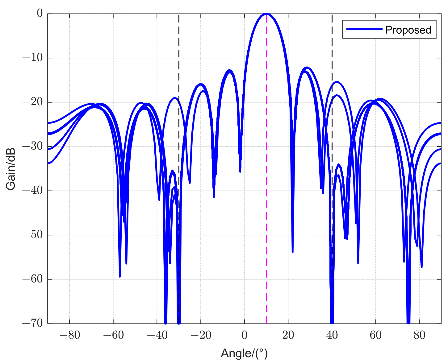
The performance of a beamformer is typically assessed in terms of its beampattern and output signal-to-interference-plus-noise ratio (SINR). The beampattern is a function directly related to spatial information, giving a more intuitive understanding of how the beamformer receives signals from different spatial directions. Ideally, the major lobe of the array pattern should be aligned with the direction of the desired signal, with all interference falling into nulls, and the deeper the nulls, the stronger the interference suppression capability. The output SINR is the ratio of the desired signal power to the total power of the interference plus noise in the beamformer’s output, which is a primary metric for evaluating beamformer performance. Under the same conditions, a beamformer with a higher output SINR has better capability to suppress interference and noise.

5.3.1. Beampattern

The following Figure 5 and Figure 6 present the simulated beampattern of various algorithms under an input SNR of 20 dB and an SIR of −3 dB, respectively. The black dotted lines in the figures represent the actual DOA of the DME signals, and the pink dotted line represents the actual DOA of the OFDM signal. The arrows in Figure 6 indicate magnified views of specific areas. Figure 5 illustrates the beampattern of the proposed algorithm based on 50 Monte Carlo trials, and Figure 6 contrasts the beampattern between the proposed and other algorithms. These simulations demonstrate that the proposed algorithm can accurately align its main lobe with the OFDM signal. In contrast, the main lobes of the INCM-subspace and INCM-volume algorithms do not precisely align with the direction of the OFDM signal. Furthermore, the proposed algorithm forms deeper nulls in the directions of the two DME signals compared to the other two algorithms.

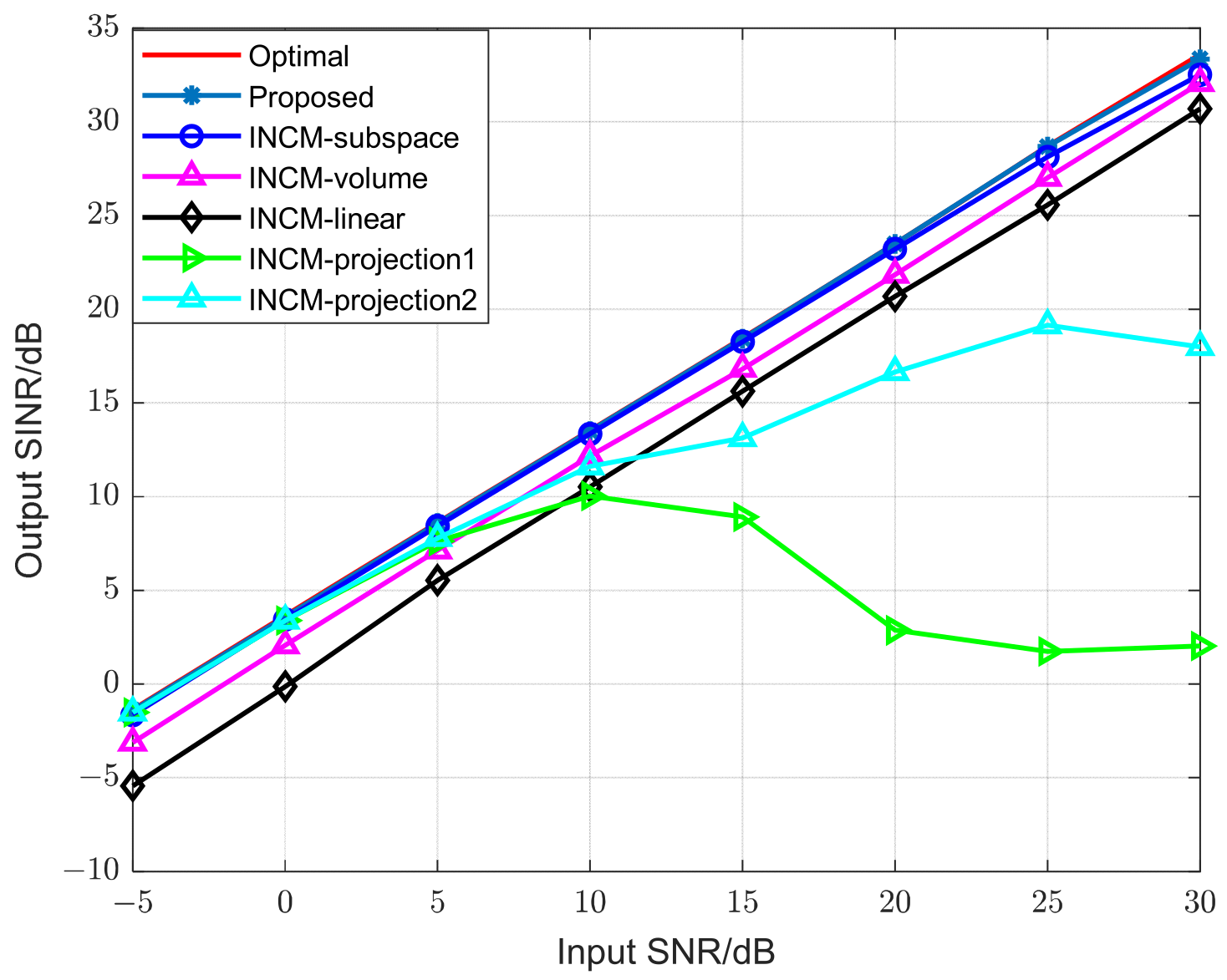
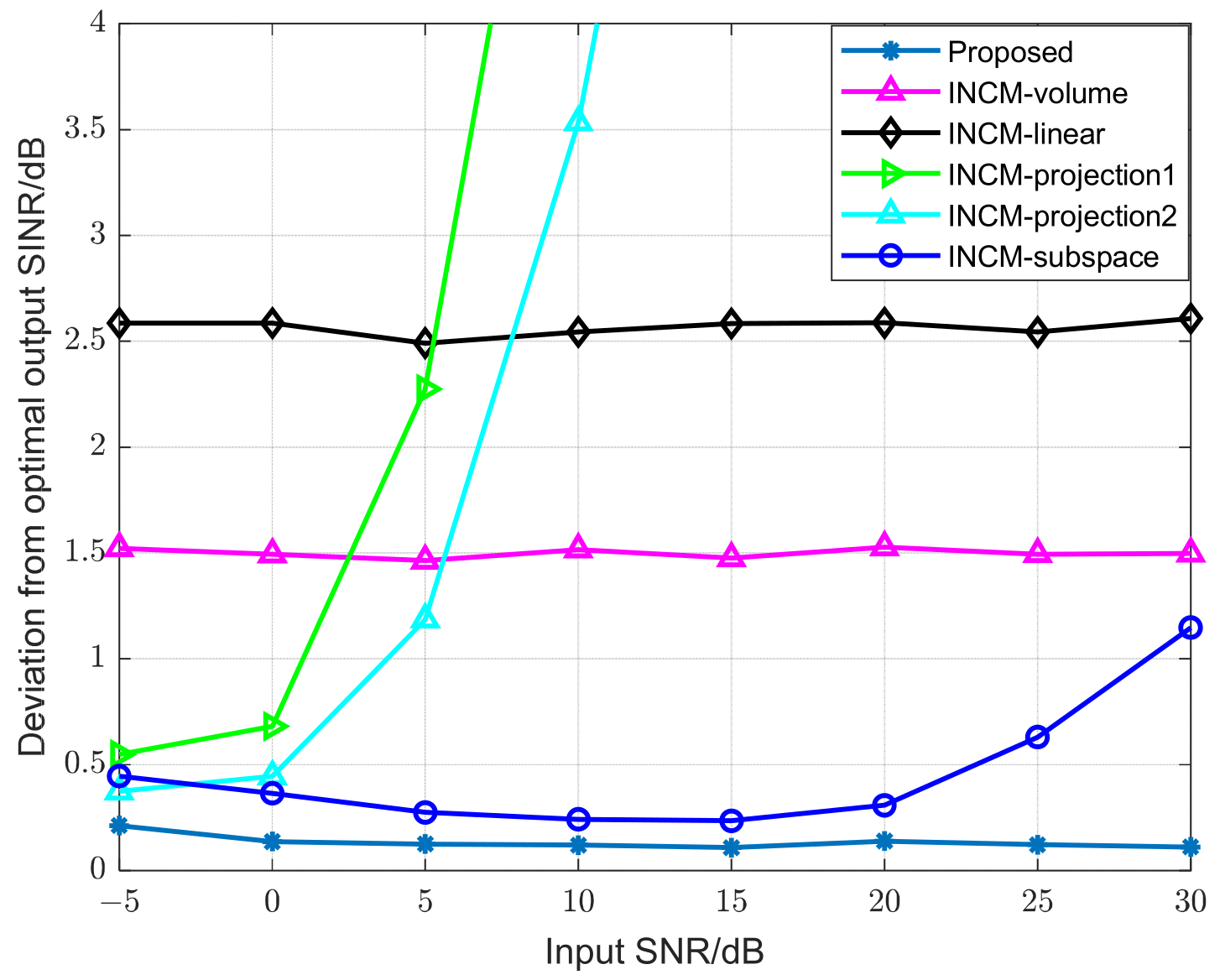
5.3.2. Relationship between Output SINR and Input SNR

In order to further compare and study the performance of the beamformer proposed in this paper, the output SINR under a different OFDM signal input SNR is simulated, and 100 Monte Carlo experiments are conducted independently for each SNR, and the simulation results are shown in Figure 7. To more intuitively analyze the performance gap of each algorithm compared to the optimal beamformer, Figure 8 makes the deviation graph of the output SINR of each beamformer from that of the optimal beamformer.

As can be seen from Figure 7 and Figure 8, the algorithm proposed in this paper is the closest to the optimal algorithm under both high and low SNR conditions. In addition to this, the INCM-subspace algorithm also has a better performance, but at higher SNRs, it starts to suppress the desired signal, leading to a performance decline. The INCM-volume algorithm and the INCM-linear algorithm are more stable but with relatively poor performance, and the INCM-projection1 and INCM-projection2 algorithms have a sharp drop in performance at SNRs greater than 0 due to the incomplete removal of OFDM signal components. Thus, it can be seen that the algorithm in this paper not only has a better performance but also has stronger robustness.

5.3.3. Relationship between Output SINR and DOA Estimation Error

To verify the impact of DOA estimation accuracy on each beamforming algorithm, simulations are conducted to compare the output SINR under different error conditions. Figure 9 below compares the performance of various algorithms with the OFDM signal DOA estimation errors within $\left[-4°, 4°\right]$ conditions, where the SNR is set to 20 dB and each group undergoes 100 Monte Carlo experiments. The figure shows that algorithms like INCM-subspace, INCM-volume, INCM-linear, INCM-projection2, and the algorithm proposed in this paper maintain a linear relationship between SINR and DOA error, which indicates that these algorithms can effectively resist the DOA estimation error in a certain range. In contrast, the INCM-projection1 algorithm has a sharp decrease in performance after the DOA estimation error, in the absolute value, exceeds 2°.

5.3.4. Relationship between Output SINR and Number of Snapshots

Figure 10 shows the output SINR of each algorithm with the number of snapshots at an input SNR of 20 dB, with 100 Monte Carlo experiments for each group, and it can be seen that most of the algorithms have a stable performance with varying numbers of snapshots. Although the proposed algorithm’s performance at fewer snapshots is slightly lower than the INCM-subspace algorithm, it approaches the optimal algorithm most closely when the number of snapshots reaches 170 and above.

5.4. BER Performance

To thoroughly evaluate the effectiveness of the proposed method for LDACS, we conducted BER simulations and contrasted its performance with that of other algorithms. BER quantifies the ratio of error bits to total transmitted bits, serving as a direct indicator of a system’s reliability and communication quality, making it a vital metric for a comprehensive evaluation of communication systems.

Figure 11 simulates the BER variation with SNR for various algorithms. Using the curve, which lacks interference suppression, as a baseline, it is clear that all simulated algorithms demonstrate improvements in BER to varying extents across different SNR levels. Notably, as shown in Figure 11, the proposed method consistently outperforms the other methods across a broad range of SNR values. Furthermore, the figure reveals a significant improvement in BER performance at lower SNRs, highlighting the proposed method’s enhanced capability to maintain signal integrity in challenging noise environments. These results demonstrate that the proposed method not only improves signal detection and suppression but also significantly improves the overall reliability and quality of LDACS communications.

5.5. Comparison of Running Time of Each Algorithm

Table 3. Average running time for a single Monte Carlo simulation.

Algorithm	Running Time/Second
Proposed	0.063519
INCM-volume	0.690478
INCM-linear	0.263194
INCM-projection1	0.022785
INCM-projection2	0.528757
INCM-subspace	0.018252

summarizes the average runtime of a single Monte Carlo simulation for the six INCM reconstruction-based beamforming algorithms mentioned above. All simulations are conducted under the same conditions. Combining Table 1 and Table 3, it is evident that, among these similarly performant beamforming algorithms, such as INCM-projection2 and INCM-volume, the algorithm proposed in this paper has lower complexity. Although the complexity of INCM-subspace and INCM-projection1 is lower, the proposed algorithm is easier to implement and has a better performance.

6. Conclusions

In this paper, the proposed method significantly mitigates the DME interference in LDACS signal reception, as verified by comprehensive simulation experiments. By employing the Cyclic-MUSIC algorithm for precise DOA estimation and using the INCM reconstruction method for beamforming, our approach effectively suppresses the impact of DME signals on OFDM receiver. Quantitative analysis reveals the algorithm’s superior performance in forming a high-gain main lobe towards the OFDM signal and deep nulls at interference points, which is evident in the improved output SINR across various scenarios. Compared to existing algorithms based on INCM reconstruction, the proposed method not only demonstrates lower computational complexity and higher beamforming robustness but also achieves a lower BER, making it a promising solution for advanced interference mitigation in aeronautical communications.

References

1. Global Market Forecast|Airbus. Available online: https://www.airbus.com/en/products-services/commercial-aircraft/market/global-market-forecast (accessed on 7 March 2024).
2. Zhou, J.; Dan, Z.; Wang, Y.; Wang, S.; Wang, Z. Impact of DME Interference on LDACS Channel Estimation in En-route Phase. In Proceedings of the 2023 IEEE/AIAA 42nd Digital Avionics Systems Conference (DASC), Barcelona, Spain, 1–5 October 2023; pp. 1–6. [Google Scholar]
3. EUROCONTROL Forecast Update 2023–2029|EUROCONTROL. Available online: https://www.eurocontrol.int/publication/eurocontrol-forecast-update-2023-2029 (accessed on 7 March 2024).
4. Schnell, M.; Epple, U.; Shutin, D.; Schneckenburger, N. LDACS: Future aeronautical communications for air-traffic management. IEEE Commun. Mag. 2014, 52, 104–110. [Google Scholar] [CrossRef]
5. Agrawal, N.; Ambede, A.; Darak, S.J.; Vinod, A.P.; Madhukumar, A.S. Design and Implementation of Low Complexity Reconfigurable Filtered-OFDM-Based LDACS. IEEE Trans. Circuits Syst. II Express Briefs 2021, 68, 2399–2403. [Google Scholar] [CrossRef]
6. Bellido-Manganell, M.A.; Gräupl, T.; Heirich, O.; Mäurer, N.; Filip-Dhaubhadel, A.; Mielke, D.M.; Schalk, L.M.; Becker, D.; Schneckenburger, N.; Schnell, M. LDACS Flight Trials: Demonstration and Performance Analysis of the Future Aeronautical Communications System. IEEE Trans. Aerosp. Electron. Syst. 2022, 58, 615–634. [Google Scholar] [CrossRef]
7. Qian, L.; Xu, H.; Wang, L.; Wang, D.; Liu, X.; Shi, B. Physical Layer Security for L-Band Digital Aeronautical Communication System with Interference Mitigation. Electronics 2023, 12, 4591. [Google Scholar] [CrossRef]
8. Muthalagu, R. Mitigation of DME interference in LDACS1-based future air-to-ground (A/G) communications. Cogent Eng. 2018, 5, 1472199. [Google Scholar] [CrossRef]
9. Epple, U.; Schnell, M. Advanced Blanking Nonlinearity for Mitigating Impulsive Interference in OFDM Systems. IEEE Trans. Veh. Technol. 2017, 66, 146–158. [Google Scholar] [CrossRef]
10. Zhidkov, S.V. Performance analysis and optimization of OFDM receiver with blanking nonlinearity in impulsive noise environment. IEEE Trans. Veh. Technol. 2006, 55, 234–242. [Google Scholar] [CrossRef]
11. Epple, U.; Shutin, D.; Schnell, M. Mitigation of Impulsive Frequency-Selective Interference in OFDM Based Systems. IEEE Wirel. Commun. Lett. 2012, 1, 484–487. [Google Scholar] [CrossRef]
12. Zhidkov, S.V. Analysis and comparison of several simple impulsive noise mitigation schemes for OFDM receivers. IEEE Trans. Commun. 2008, 56, 5–9. [Google Scholar] [CrossRef]
13. Liu, H.; Cheng, W.; Zhang, X. DME Pulse Interference Mitigation Method Based on Joint Orthogonal Transform and Signal Interleaving. Acta Aeronaut. Astronaut. Sin. 2014, 35, 1365–1373. [Google Scholar] [CrossRef]
14. Chen, C.; Zhuo, Y. A research on anti-jamming method based on compressive sensing for OFDM analogous system. In Proceedings of the 2017 IEEE 17th International Conference on Communication Technology (ICCT), Chengdu, China, 27–30 October 2017; pp. 655–659. [Google Scholar]
15. Saaifan, K.A.; Elshahed, A.M.; Henkel, W. Cancelation of Distance Measuring Equipment Interference for Aeronautical Communications. IEEE Trans. Aerosp. Electron. Syst. 2017, 53, 3104–3114. [Google Scholar] [CrossRef]
16. Odhah, N.A.; Hassan, E.S.; Abdelnaby, M.; Al-Hanafy, W.E.; Dessouky, M.I.; Alshebeili, S.A.; Abd El-Samie, F.E. Adaptive Resource Allocation Algorithms for Multi-user MIMO-OFDM Systems. Wirel. Pers. Commun. 2015, 80, 51–69. [Google Scholar] [CrossRef]
17. Odhah, N.A.; Hassan, E.S.; Dessouky, M.I.; Al-Hanafy, W.E.; Alshebeili, S.A.; Abd El-Samie, F.E. Adaptive Per-spatial Stream Power Allocation Algorithms for Single-User MIMO-OFDM Systems. Wirel. Pers. Commun. 2018, 98, 1–31. [Google Scholar] [CrossRef]
18. Liu, H.; Liu, Y.; Zhang, X. Interference mitigation method based on joint DOA estimation and main beam forming. J. Harbin Inst. Technol. 2016, 48, 103–108. [Google Scholar] [CrossRef]
19. Liu, H.; Liu, Y.; Zhang, X. DME Impulse Interference Mitigation Method Based on Subspace Projection and CLEAN Algorithm. J. Signal Process. 2015, 31, 536–543. [Google Scholar] [CrossRef]
20. Du, L.; Li, J.; Stoica, P. Fully Automatic Computation of Diagonal Loading Levels for Robust Adaptive Beamforming. IEEE Trans. Aerosp. Electron. Syst. 2010, 46, 449–458. [Google Scholar] [CrossRef]
21. Li, J.; Stoica, P.; Wang, Z. On robust Capon beamforming and diagonal loading. IEEE Trans. Signal Process. 2003, 51, 1702–1715. [Google Scholar] [CrossRef]
22. Huang, F.; Sheng, W.; Ma, X. Modified projection approach for robust adaptive array beamforming. Signal Process. 2012, 92, 1758–1763. [Google Scholar] [CrossRef]
23. Jia, W.; Jin, W.; Zhou, S.; Yao, M. Robust adaptive beamforming based on a new steering vector estimation algorithm. Signal Process. 2013, 93, 2539–2542. [Google Scholar] [CrossRef]
24. Zhu, X.; Ye, Z.; Xu, X.; Zheng, R. Covariance Matrix Reconstruction via Residual Noise Elimination and Interference Powers Estimation for Robust Adaptive Beamforming. IEEE Access 2019, 7, 53262–53272. [Google Scholar] [CrossRef]
25. Zheng, Z.; Zheng, Y.; Wang, W.-Q.; Zhang, H. Covariance Matrix Reconstruction With Interference Steering Vector and Power Estimation for Robust Adaptive Beamforming. IEEE Trans. Veh. Technol. 2018, 67, 8495–8503. [Google Scholar] [CrossRef]
26. Zhu, X.; Xu, X.; Ye, Z. Robust adaptive beamforming via subspace for interference covariance matrix reconstruction. Signal Process. 2020, 167, 107289. [Google Scholar] [CrossRef]
27. Gu, Y.; Leshem, A. Robust Adaptive Beamforming Based on Interference Covariance Matrix Reconstruction and Steering Vector Estimation. IEEE Trans. Signal Process. 2012, 60, 3881–3885. [Google Scholar] [CrossRef]
28. Gardner, W. Spectral Correlation of Modulated Signals: Part I—Analog Modulation. IEEE Trans. Commun. 1987, 35, 584–594. [Google Scholar] [CrossRef]
29. Yang, H.; Ye, Z. Robust Adaptive Beamforming Based on Covariance Matrix Reconstruction via Steering Vector Estimation. IEEE Sens. J. 2023, 23, 2932–2939. [Google Scholar] [CrossRef]
30. Hassanien, A.; Vorobyov, S.A.; Wong, K.M. Robust Adaptive Beamforming Using Sequential Quadratic Programming: An Iterative Solution to the Mismatch Problem. IEEE Signal Process. Lett. 2008, 15, 733–736. [Google Scholar] [CrossRef]
31. Yuan, X.; Gan, L. Robust adaptive beamforming via a novel subspace method for interference covariance matrix reconstruction. Signal Process. 2017, 130, 233–242. [Google Scholar] [CrossRef]
32. Huang, L.; Zhang, J.; Xu, X.; Ye, Z. Robust Adaptive Beamforming With a Novel Interference-Plus-Noise Covariance Matrix Reconstruction Method. IEEE Trans. Signal Process. 2015, 63, 1643–1650. [Google Scholar] [CrossRef]
Figure 1. Block diagram of OFDM receiver for LDACS system.
Electronics 13 01600 g001
Figure 2. Power spectrum of Cyclic-MUSIC algorithm at SNR = −5 dB.
Electronics 13 01600 g002
Figure 3. Power spectrum of Cyclic-MUSIC algorithm at SNR = 20 dB.
Electronics 13 01600 g003
Figure 4. RMSE versus SNR curve.
Electronics 13 01600 g004
Figure 5. Beampattern diagram.
Electronics 13 01600 g005
Figure 6. Gain comparison of different algorithm beamformers.
Electronics 13 01600 g006
Figure 7. Output SINR versus SNR.
Electronics 13 01600 g007
Figure 8. Deviation of different algorithms from the optimal output SINR.
Electronics 13 01600 g008
Figure 9. Output SINR versus DOA error angles.
Electronics 13 01600 g009
Figure 10. Output SINR of the adaptive beamformer for (a) 100~200 snapshots and (b) 100~1000 snapshots.
Electronics 13 01600 g010
Figure 11. BER versus SNR curve.
Electronics 13 01600 g011