Explaining Misinformation Detection Using Large Language Models

Abstract

Large language models (LLMs) are a compressed repository of a vast corpus of valuable information on which they are trained. Therefore, this work hypothesizes that LLMs such as Llama, Orca, Falcon, and Mistral can be used for misinformation detection by making them cross-check new information with the repository on which they are trained. Accordingly, this paper describes the findings from the investigation of the abilities of LLMs in detecting misinformation on multiple datasets. The results are interpreted using explainable AI techniques such as Local Interpretable Model-Agnostic Explanations (LIME), SHapley Additive exPlanations (SHAP), and Integrated Gradients. The LLMs themselves are also asked to explain their classification. These complementary approaches aid in better understanding the inner workings of misinformation detection using LLMs and lead to conclusions about their effectiveness at the task. The methodology is generic and nothing specific is assumed for any of the LLMs, so the conclusions apply generally. Primarily, when it comes to misinformation detection, the experiments show that the LLMs are limited by the data on which they are trained.

1. Introduction

Large language models (LLMs) are known to hallucinate and produce misinformation. This work hypothesizes that the same LLMs can be used to detect misinformation. In this paper, several LLMs are compared for their ability to detect misinformation, while interpreting the results using explainable AI techniques such as LIME, SHAP, and Integrated Gradients.

With their high level of Natural Language Understanding, LLMs have proven to be exceptionally versatile and able to accomplish many tasks without fine-tuning gradient updates [1]. Despite these strengths, LLMs are prone to hallucinations and exploitation, sometimes producing output ranging from wrong to offensive to nonsensical. Yet, LLMs also have a track record of being applied to various tasks, ranging from translation to question answering, and setting new records on these benchmarks [1]. Therefore, in this paper, the idea of explaining the behavior of LLMs in detecting misinformation is explored. Specifically, the following questions are investigated:

• RQ1: How do various large language models (LLMs) compare when detecting misinformation?
• RQ2: Why do the LLMs differ in their abilities to detect misinformation from an explainability perspective?

Depending merely on machine learning evaluation metrics such as accuracy, precision, and recall to rely on the model’s performance can be misleading [2]. It is important to corroborate the results using explainable AI techniques. This work therefore uses LIME, SHAP, and Integrated Gradients to assess the LLMs’ performance in detecting misinformation.

1.1. Related Work

Misinformation containment has been investigated extensively and significant successes using machine learning have been claimed despite the problem being largely unsolved [3]. A spectral analysis of the embeddings generated by language models revealed interesting insights into why the problem is still unsolved [4]. There are numerous online datasets, including the classic LIAR [5] dataset and more recent datasets such as the COVID-19 dataset [6]. This paper uses both datasets for the experiments. The work that published the LIAR dataset [5] used a hybrid CNN for misinformation detection. On the other hand, the research corresponding to the COVID-19 dataset [6] used several traditional machine learning approaches such as Decision Tree, Logistic Regression, Gradient Boosting, and Support Vector Machine (SVM). More recent approaches [7] have integrated newer technologies, including the use of pre-trained transformers such as BERT [8] and XLNet [9].

There seems to be substantial work conducted to mitigate the LLM hallucinations [10] but there is hardly any work on the use of large language models for misinformation detection when compared with the use of smaller language models. A recent work to utilize ChatGPT 3.5 to classify multi-modal misinformation in a binary context [11] mentioned that it was limited in the scope of its study. It uses only a small sample size. Recent work has attempted to use ChatGPT 3.5 on misinformation datasets in Chinese and English [12], noting that even when given Chain of Thought (CoT) prompts, ChatGPT underperformed in fine-tuning small language models.

Moreover, these works focus only on ChatGPT. While certainly one of the most accessible LLMs today, ChatGPT is by no means the only LLM available. Other LLMs include Microsoft’s Orca, Google’s PaLM and Gemini, Meta’s LLaMa family [13], the Falcon family [14], as well as Mistral [15], among many others. On relevant benchmarks, including TruthfulQA [16], several of these LLMs perform similarly to GPT4 when compared using HuggingFace’s Open LLM leaderboard [17]. The existing literature therefore prompts discussion on how the various LLMs perform when used for the task of misinformation detection and classification, leading to the research questions listed earlier.

For better understanding, there is also a need to analyze the performance of the LLMs in this domain using explainable AI (XAI). Explainability in AI has been a fundamental issue for a long time. Numerous methods such as feature ablation [18], LIME [19], Integrated Gradients [20], and SHAP [21] have been proposed to provide explanations for the machine learning models’ behavior. Perturbation-based methods, such as LIME and SHAP, adjust model inputs to determine which are most responsible for the output. Meanwhile, gradient-based approaches, such as Integrated Gradients, attempt to use gradients reflecting how fast the models’ outputs change to indicate which input features are most responsible for the output.

OpenAI has explored the possibility of using ChatGPT to explain its neurons [22] and the role they play in generating outputs. A literature survey did not reveal a substantial amount of literature on using traditional explainability techniques such as LIME and SHAP on LLMs.

1.2. Contribution of the Paper

LLMs hold a huge potential to play an important role in various aspects of day-to-day life. This work hypothesizes that in the future, they will play a major role in misinformation containment as well. The work presented in this paper, to the best of our knowledge, is unique in assessing and using explainable AI techniques and interpreting the performance of LLMs in detecting misinformation. The findings are interesting and segue into an important application domain for LLMs—that of misinformation containment.

2. Materials and Methods

The first and second research questions have been addressed, respectively, using the quantitative and qualitative methods described in the next few paragraphs. The second question is addressed using a qualitative approach due to the nature of the explainability problem. Explainability algorithms can quantitatively emphasize certain attributes in the input features that the models focus on, but human interpretations of those highlighted aspects are qualitative.

The approach primarily comprises prompting LLMs to classify information in datasets as true or false or a degree between the two. The datasets already contain the correct classifications. The accuracy of the LLMs in detecting misinformation can be computed by comparing the predicted and correct classifications, similar to how it is performed in machine learning classification projects. The predicted classifications are then explained using post hoc explainability methods, LIME, SHAP, and Integrated Gradients. LLMs are also asked to explain their classifications. The explanations from the LLMs and the post hoc explainability methods are compared to understand the LLM behavior when it comes to misinformation detection. The flow schematic is described in Figure 1.

Concerning the methods used, two overtures are in order. Deep learning models normally use high-precision data types, such as 32-bit floating-point numbers, abbreviated as float32, to store and compute their weights and activations. To reduce the memory footprint and improve the inferencing speed, a technique called quantization is typically used. The technique converts float32 parameters into a lower-precision format such as 8-bit integers (int8) or 4-bit integers (int4). Using fewer bits to store the parameters significantly reduces the memory needed to store and run the model. Therefore, unless otherwise stated, 4-bit float (fp4) quantization was used for all the experiments detailed in this paper to reduce our models’ memory footprint and allow the experiments to run efficiently on a single GPU.

Normally, LLMs pick the next word based on the probabilities assigned by the model. This is the basis for the technique called sampling. It makes the process stochastic and the outputs probabilistic. This implies that different outputs are generated each time the model is run. If sampling is not used, the LLM chooses the next word according to its internal understanding. This is a greedy approach as the LLM algorithm picks the most optimal option at each step, without regard to the long-term consequences. In this greedy approach, since the model is not making random choices, the outputs generated for a given prompt are the same even when asked multiple times. For the experiments described in this paper, unless stated otherwise, the models were made to generate text without sampling, equivalent to greedy decoding, so that deterministic outputs are produced.

2.1. Quantitative Experiments

For the first research question, the misinformation detection capabilities of Mistral [15], Llama2 [13], Microsoft’s fine-tuned Orca version [23], and Falcon [14] were explored. Prompting in the context of large language models (LLMs) is the process by which we give instructions to the model to carry out a particular task. Zero-shot and few-shot prompting are two popular methods for guiding LLMs. Zero-shot prompting involves giving the LLM precise directions without providing any examples of how the work should be accomplished. This method depends on the LLM’s capacity to comprehend instructions, adhere to them, and use its internal knowledge to finish the task. On the other hand, few-shot prompting is analogous to setting an example for the LLM. This method is akin to providing the LLM with a few examples to demonstrate the desired outcome. The LLM is given a prompt that describes the work and the intended result, as well as a limited number of examples, usually one to five, that show them how to perform the task. These illustrations aid in the LLM’s understanding of the task’s subtleties and increase the precision of its outputs.

The experiments used both zero-shot and few-shot prompting strategies to obtain a more holistic view of model performance. Few-shot examples were sampled randomly from the corresponding dataset for LLM’s comprehension. These samples were excluded from the dataset used to evaluate the model’s accuracy. The algorithm for evaluating each model’s accuracy is detailed in Algorithm 1. Accuracy is computed as follows:

$$Accuracy=\frac{numberofsamplescorrectlyclassifiedbytheLLM}{(Sizeofthedataset-numberofsamplesusedasfewshots}$$

Algorithm 1 LLM performance evaluation
$i\leftarrow 0$
$correct\leftarrow 0$
while $i\ne \left|Dataset\right|$ do	▹ For each sample in the dataset
if $i\notin Examples$ then	▹ If it is not in the few-shot examples used
$generation\leftarrow \mathtt{m}\mathtt{o}\mathtt{d}\mathtt{e}\mathtt{l}.\mathtt{g}\mathtt{e}\mathtt{n}\mathtt{e}\mathtt{r}\mathtt{a}\mathtt{t}\mathtt{e}\left(Dataset\right[i\left]\right)$	▹ Generate the classification
if $generation=Dataset\left[i\right]{[}^{\prime }labe{l}^{\prime }]$ then
	▹ If the label matches what is in the dataset
$correct\leftarrow correct+1$
	▹ Increment the number of correctly classified samples
end if
end if
$i\leftarrow i+1$	▹ Proceed to the next sample
end while
$accuracy\leftarrow correct÷\left(\right|Dataset|-|Examples\left|\right)$
▹ In the denominator, subtract the samples used as few-shots from the size of the dataset

In addition to the accuracy, the F1-score, Matthew’s correlation coefficient (MCC), and Cohen’s Kappa score [24] were also computed for all the experiments. These metrics are generally considered to be effective even for imbalanced datasets. MCC is particularly recommended for binary classification in all scientific domains [25].

Matthew’s correlation coefficient, MCC, is given by the following formula:

$$\mathit{MCC}=\frac{(\mathit{TP}·\mathit{TN}-\mathit{FP}·\mathit{FN})}{\sqrt{(\mathit{TP}+\mathit{FP})·(\mathit{TP}+\mathit{FN})·(\mathit{TN}+\mathit{FP})·(\mathit{TN}+\mathit{FN})}}$$

where ($\mathit{TP}$) is True Positive; ($\mathit{TN}$) is True Negative; ($\mathit{FP}$) is False Positive; and ($\mathit{FN}$) is False Negative.

A comprehensive set of metrics and results is tabulated in Appendix B.

2.2. Misinformation Detection in the COVID-19 Dataset

The COVID-19 dataset [6] used for the first set of experiments contains 10,700 social media posts and articles related to COVID-19, labeled as real or fake news. The dataset contains conjecture and false information regarding COVID-19 gathered from fact-checking websites, along with actual news from recognized Twitter accounts like those of the CDC and the WHO. The information is manually checked and annotated as authentic or fraudulent. There are 52.34% actual news and 47.66% fake news samples in the dataset, making it a fairly balanced dataset. Real posts average 31.97 words, whereas false posts average 21.65 words. The total number of terms in the vocabulary is 37,503. Using machine learning models such as SVM, Logistic Regression, Decision Trees, and Gradient Boosting, the authors benchmarked the dataset. On the test set, SVM had the best F1-score of 93.32% for differentiating between fake and authentic news. The algorithm and dataset are available to the public to further study automatically detecting fake news.

For the experiments in this paper, the models were given a multiple-choice question that prompted them to give a binary response as to whether a given claim was true or false.

2.3. Prompting Strategy for the COVID-19 Dataset

Each entry within the dataset contained the following fields:

• id;
• tweet;
• label.

The information snippets in the dataset were truncated to a maximum length of 256 tokens before converting each entry into a prompt in the following format:

Please select the option (A or B) that most closely describes the following claim: {truncated tweet}.

(A) True

(B) False

Choice: (

The reason for the ( at the end of each prompt strategy was to prevent the undesired behavior of models starting a new line and then elaborating on a response without giving a single-letter answer. It was determined that by adding the (, most models responded with a letter answer as the first new token.

No system prompts were prepended to the prompts. For few-shot prompts, the target question was formatted as mentioned above and the examples were similarly provided to the LLM. The few-shot examples contained the single-letter answer for the given example, closing parentheses, and two ending newlines.

2.4. Accuracy Computation for the COVID-19 Dataset

The performance of the models is summarized in

Table 1. Model performance on the COVID-19 dataset.

	LLama2-7b	Falcon-7b	Mistral-7b	Orca-7b	Avg
Zero-Shot	58.15%	49.72%	80.75%	60.50%	62.28
1-Shot	54.10%	39.44%	82.01%	57.60%	58.29
5-Shot	57.35%	52.33%	83.04%	80.69%	68.35

and

Table 2. Multi-class classification metrics for models evaluated on the COVID-19 dataset in a binary classification setting.

	Precision	Recall	F1	MCC	Kappa
0-Shot COVID
Orca	0.661	0.578	0.526	0.225	0.162
Falcon	0.465	0.500	0.346	−0.008	−0.001
Llama	0.600	0.599	0.596	0.199	0.197
Mistral	0.684	0.649	0.638	0.331	0.303
1-Shot COVID
Orca	0.656	0.531	0.425	0.140	0.065
Falcon	0.428	0.437	0.414	−0.135	−0.123
Llama	0.618	0.532	0.417	0.123	0.061
Mistral	0.688	0.686	0.687	0.374	0.373
5-Shot COVID
Orca	0.692	0.670	0.665	0.361	0.344
Falcon	0.262	0.500	0.344	−0.009	−0.000
Llama	0.621	0.554	0.472	0.161	0.104
Mistral	0.712	0.692	0.689	0.404	0.389

. The former lists the accuracy and the latter lists a more exhaustive set of metrics.

Curiously, Mistral outperforms its competitors immensely when it comes to detecting COVID-19-related misinformation. When given 5-shot prompts, Orca performed similarly to Mistral, perhaps because those prompts better establish the context of the problem. However, Orca’s performance on 1-shot and 0-shot prompts is drastically less than Mistral’s. Meanwhile, Falcon’s performance is consistently the lowest, with an average accuracy of 47.16%, less than it would have achieved from randomly guessing. Similarly, the performance of Llama is only slightly better than random chance.

2.5. Misinformation Detection in the LIAR Dataset

Finding the differences in their performance intriguing, the next set of experiments was performed on the LIAR dataset [5]. The LIAR dataset is made up of a set of assertions with labels indicating their veracity. It includes about 12,800 brief quotes taken from the fact-checking website PolitiFact.com about political claims. On a scale ranging from “pants on fire”, which indicates utter falsity, to “true”, each statement is given a label that indicates its degree of veracity. The dataset is accessible to the general public and can be used to train machine learning models that identify false information.

Similarly to how it was conducted with the COVID-19 dataset, each entry is converted into a multiple-choice question for easy grading. However, instead of binary classification, the models were asked to classify the given statement as one of the 6 labels in the LIAR dataset, namely “True”, “Mostly True”, “Half True”, “Barely True”, “False”, and “Pants on Fire”. These labels comprise 16.1%, 19.2%, 20.5%, 16.4%, 19.6%, and 8.2%, respectively, of the dataset. Later, we convert the dataset to the binary labels True and False, which comprise 55.8% and 44.2%, respectively, of the dataset.

2.5.1. Prompt Strategy for the LIAR Dataset

Each entry in the LIAR dataset contained the following fields:

• id;
• label;
• statement;
• subject;
• speaker;
• job_title;
• state_info;
• party_affiliation;
• barely_true_counts;
• false_counts;
• half_true_counts;
• mostly_true_counts;
• pants_on_fire_counts;
• context.

Each entry would then be converted into a prompt of the following format:

Please select the option that most closely describes the following claim by {speaker}:

{statement}

A) True

B) Mostly True

C) Half True

D) Barely True

E) False

F) Pants on Fire (absurd lie)

Choice: (

2.5.2. Performance of the LLMs on the LIAR Dataset

Based on its performance on the COVID-19 dataset, Mistral was expected to exhibit a similar stellar performance. Intriguingly, the results proved to be significantly different. All the LLMs perform poorly on the LIAR dataset, barely outperforming random chance. These results appear to contradict the results of prior research in the literature that proved LLMs to be extremely capable of detecting misinformation [11]. Perhaps more surprising is the fact that although 1-shot prompting outperformed zero-shot prompting, 5-shot prompting underperformed both 1-shot prompting and 5-shot prompting. These numbers did not change drastically even when providing the context and party affiliation in our prompts. The results are summarized in

Table 3. Model accuracy on the LIAR dataset.

	Llama2-7b	Falcon-7b	Mistral-7b	Orca-7b	Avg
Zero-Shot	20.15%	19.36%	22.20%	16.61%	19.58
1-Shot	21.46%	19.21%	22.84%	20.83%	21.01
5-Shot	17.72%	19.12%	22.53%	12.08%	17.86

.

A more detailed set of metrics is presented in

Table 4. Multi-class classification metrics for models run with deterministic outputs on the LIAR dataset.

	Precision	Recall	F1	MCC	Kappa
0-Shot
Orca	0.295	0.171	0.063	0.014	0.005
Falcon	0.154	0.168	0.074	0.005	0.002
Llama	0.136	0.187	0.112	0.034	0.028
Mistral	0.225	0.230	0.196	0.063	0.059
1-Shot
Orca	0.206	0.190	0.120	0.038	0.023
Falcon	0.126	0.168	0.056	0.009	0.001
Llama	0.157	0.187	0.111	0.036	0.024
Mistral	0.267	0.232	0.214	0.076	0.071
5-Shot
Orca	0.187	0.192	0.081	0.032	0.018
Falcon	0.099	0.167	0.054	0.000	0.000
Llama	0.203	0.234	0.156	0.050	0.045
Mistral	0.245	0.218	0.193	0.058	0.054

.

The distribution of the answers produced by the LLMs is shown in Figure 2. As can be seen from the figure, with the exclusion of Mistral, the answer distributions produced by the LLMs were dominated by only two answers, “B”, for “Mostly True”, and “D”, for “Barely True”. Speculating that this may be due to the LIAR dataset’s scale of True values (“Half True”, “Mostly True”, “Barely True”, “True”) and ambiguity between such labels, the experiments were repeated with binary True and False values, where “True”, “Mostly True”, and “Half True” were counted as “True”, while “Barely True”, “False”, and “Pants on Fire” were counted as “False”. Unfortunately, repeating the experiments with binary options did not yield appreciably better results. The models still barely outperformed random chance on average, as can be observed from

Table 5. LLM performance on the LIAR dataset with binary response. Percentages reflect the accuracy obtained by each model.

	Llama2-7b	Falcon-7b	Mistral-7b	Orca-7b	Avg
Zero-Shot	46.53%	44.98%	56.95%	59.78%	52.06
1-Shot	44.39%	44.15%	58.22%	56.53%	50.82
5-Shot	50.53%	47.51%	59.10%	58.71%	53.96

and Figure 3.

To test whether the LLM settings to produce deterministic outputs were the cause for skewed distributions and poor performance, the experiments were repeated by setting the LLMs for nondeterministic random sampling. While the distributions of the LLM answers were less skewed, the experiment (

Table 6. Model accuracies with nondeterministic sampling using the original 6 labels from the LIAR dataset. The accuracies are not significantly better than those of Table 3.

	Llama-2-7b	Falcon-7b	Mistral-7b	Orca-7b	Avg
Zero-Shot	18.92	14.78	21.73	17.26	18.17
1 Shot	19.78	18.42	21.97	18.81	19.74
5-Shot	14.10	18.70	21.64	13.80	17.06

) yielded similar results in terms of accuracy, with models failing to perform much better than random chance. Similarly,

Table 7. Model accuracies when models were evaluated in bfloat16 mode using the original 6 labels from the LIAR dataset. The accuracies are only slightly better than those of Table 3.

	Llama-2-7b	Falcon-7b	Mistral-7b	Orca-7b	Avg
Zero-Shot	20.43	19.44	22.46	17.72	20.01
1 Shot	14.46	16.04	24.83	21.34	19.17
5-Shot	11.98	19.21	23.61	13.85	17.16

shows that repeating experiments with half-precision 7b models failed to result in any drastic changes in model accuracy overall. This suggests that these poor results are not a random chance, but rather the result of model weights.

3. Interpretation of the Results Using Explainable AI Techniques

Given the poor performance of LLMs on the LIAR dataset, the next set of experiments explores what features LLMs were looking at when they came up with their predictions. While simply prompting an LLM for an answer is an option, we explore using known explainability techniques: Integrated Gradients, LIME, and SHAP.

3.1. Integrated Gradients

Integrated Gradients [20] is an approach that integrates the gradients of each input feature to determine the contribution of each input feature to the model’s output. In the context of the experiments, features, words, and tokens, all refer to the constituents of the prompt. Gradients serve as the attribution scores. As such, the result of integrating the gradients should equal the model’s output, and the difference between the Integrated Gradients and the model’s output with the convergence delta should give a sort of intuition on how accurate the attributions are, as described by the axioms in the original paper [20].

Sundarajan et al. [20] formally defined Integrated Gradients by the following equation: ${\mathtt{I}\mathtt{n}\mathtt{t}\mathtt{e}\mathtt{g}\mathtt{r}\mathtt{a}\mathtt{t}\mathtt{e}\mathtt{d}\mathtt{G}\mathtt{r}\mathtt{a}\mathtt{d}\mathtt{s}}_i\left(x\right)=(x_i-x_i^{\prime })\times {\int }_{\alpha =0}^1\frac{\partial F(x^{\prime }+\alpha \times (x-x^{\prime }))}{\partial x_i}d\alpha$. In the equation, $x_i$ represents the input data item and $x_i^{\prime }$ is the baseline reference item. Thus, the aim of Integrated Gradients is to comprehend the shift in the model’s output from the baseline (x’) to the actual input (x). To do so, the Integrated Gradients method uses a variable alpha $\alpha$, which ranges from 0 to 1, to progress along a straight-line path between x’ and x. Along this path, in the core equation, the gradient of the model’s output (f) with respect to the input (x) must be integrated. When proposing Integrated Gradients, Sundararajan et al. [20] also proposed a way to approximate the Integrated Gradients using Reimann sums according to the following equation, which is used in our experiments:

$${\mathtt{I}\mathtt{n}\mathtt{t}\mathtt{e}\mathtt{g}\mathtt{r}\mathtt{a}\mathtt{t}\mathtt{e}\mathtt{d}\mathtt{G}\mathtt{r}\mathtt{a}\mathtt{d}\mathtt{s}}_i^{approx}\left(x\right)::=(x_i-x_i^{\prime })\times {\sum }_{k=1}^m\frac{\partial F(x^{\prime }+\frac{k}{m}\times (x-x^{\prime }))}{\partial x_i}\times \frac{1}{m}$$

3.2. LIME

Local Interpretable Model-agnostic Explanations [19], abbreviated LIME, is another explainability approach that aims to provide localized interpretations of each feature’s contribution to the model’s output. LIME is a perturbation-based approach that produces an explanation based on the following formula:

$$\mathcal{E}\left(x\right)={\mathrm{argmin}}_{g\in G}L(f,g,{\pi }_x)+\mathsf{\Omega }\left(g\right)$$

where G is the family of explanation functions, L is a fidelity function, ${\pi }_x$ is the input features, $\mathsf{\Omega }$ is a complexity measure, and f is the function to approximate.

When proposing LIME, Ribiero et. al [19] explored using an approximation model as g, where g is trained to predict the target model’s output (f), based on which input features are removed or masked, thereby approximating how features contribute to the target model’s output as per the above equation. In the experiments for this work, Captum [26] and its implementation of LIME are used.

3.3. SHAP

SHAP [21] is another explainability approach based on the game theory concept of Shapley values, which measure each player’s contribution in a cooperative game. In a machine learning context, this translates to each feature’s contribution to the model’s output. The paper that proposed SHAP also proposed using a fixed-length kernel to approximate Shapley values [21]. The experiments use these approximate Shapley values.

3.4. Setup and Hyperparameters

For the experiments, 150 random samples were selected from the LIAR dataset. They were converted to prompts as described above. Next, the above explainability methods were run on each prompt, using their implementations in Captum library.

The Integrated Gradients method was performed in the embedding space using n_steps = 512, the number of rectangles to use in the Reimann sum approximation of the Integrated Gradients, since smaller numbers of steps lead to greater discrepancies between the Integrated Gradients and the actual model outputs. Using n_steps = 512 was sufficient to consistently reduce the convergence delta, or the difference between the sum of the attributions and the actual model outputs, to less than 10 percentage points. Increasing the number of steps to 1024 and above led to only slightly more accurate approximations at the cost of much more computing power. Therefore, for better efficiencies, all experiments used 512 steps.

LIME and SHAP were each performed with 512 perturbation samples. The approximation model used for LIME was an SKLearnLasso model with $\alpha =0.0003$. Our similarity function for token sequences was the cosine similarity of said sequences in the embedding space. Our perturbation function for LIME masked tokens whose indexes i were sampled from a discrete uniform distribution $U(1,n)$, where n is the number of tokens in the tokenized prompt. When the first token was allowed to be masked using the distribution $U(0,n)$, model outputs were sometimes NaN. This may be due to the nature of LLM tokenization creating a start token, which was determined to be crucial to maintaining meaningful outputs. The similarity function used for LIME was the cosine distance in the embedding space.

3.5. Interpretation of the Model Performance

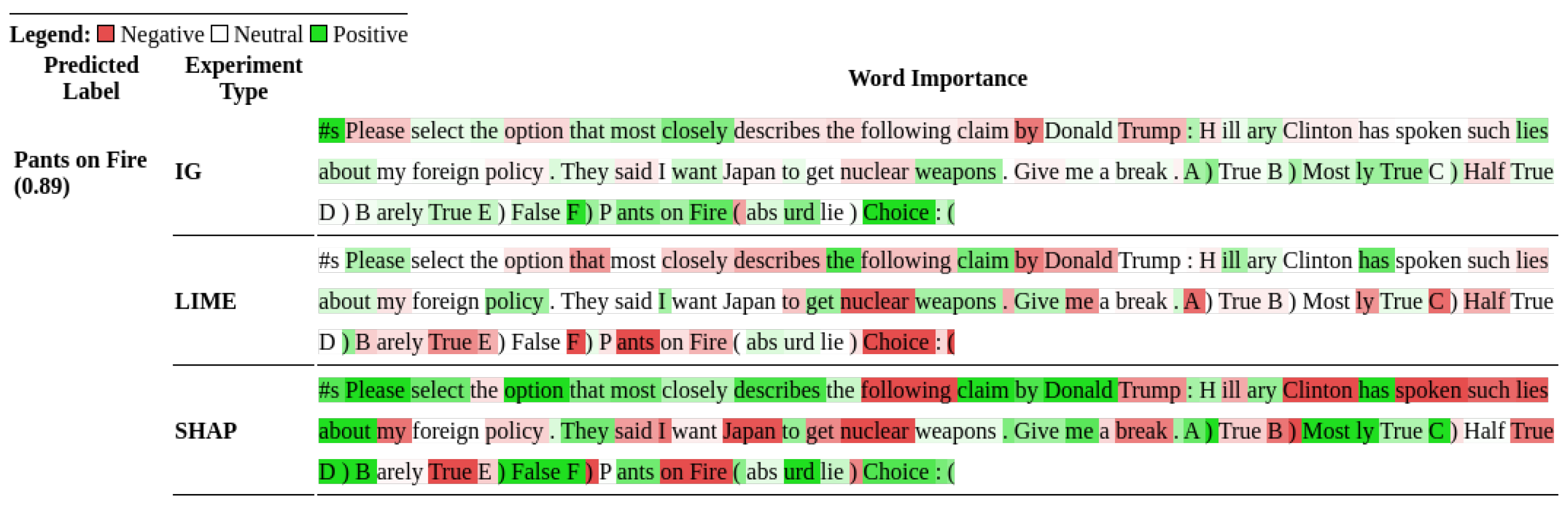
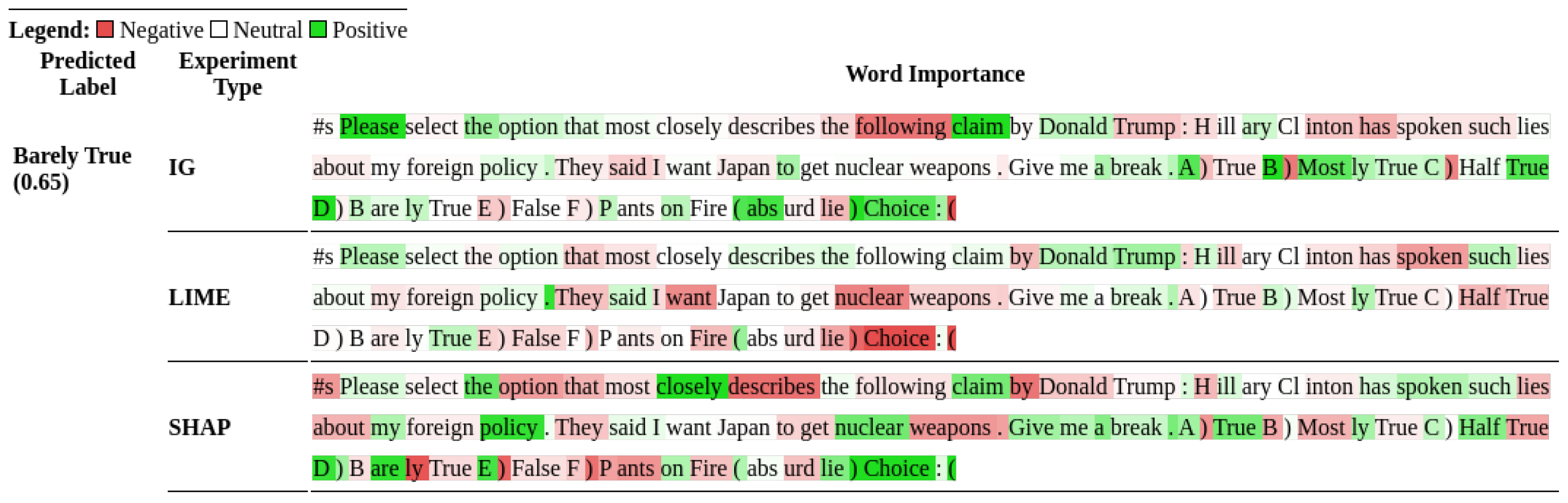
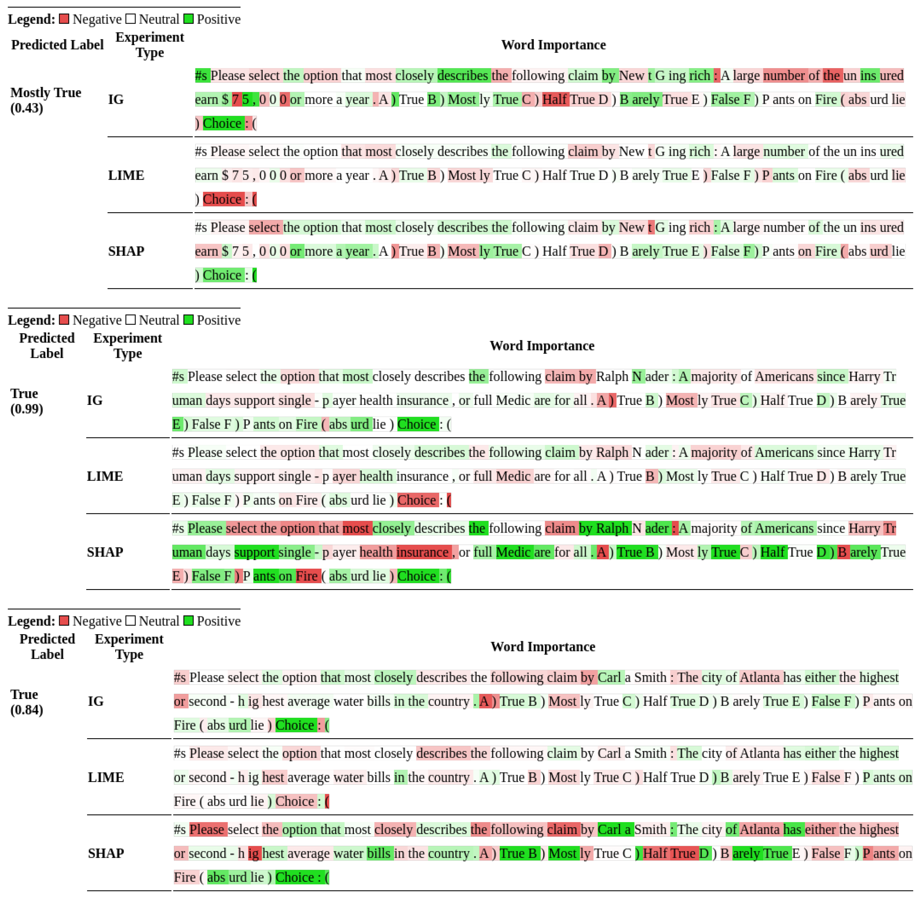
Figure 4, Figure 5, Figure 6 and Figure 7 show the output from the explainability algorithms generated for a random sample from the LIAR dataset. The figures compare the results of the different explainability techniques across different models. The figures show the classification that the model produced along with the probability attached to it. For example, Mostly True (0.07) indicates that the probability of outputting “B”, which corresponds to Mostly True, was 0.07, and the highlighted text that goes with it indicates what tokens increased or decreased that probability. The highlighted token’s impact on the overall model output is reflected in the highlight’s intensity.

The importance an LLM attaches to the words in the prompt to arrive at the classification is determined by the highlighting and the color legend. Most of the attributions in the figures seem similar to what humans would highlight if they were to classify the same claims. For instance, in Figure 4, the highlighting using SHAP shows that the LLM’s decision to classify the statement as “B) Mostly True” was positively influenced by the words highlighted in green such as “that most closely describes, Hillary, such lies, ...” and negatively influenced by “claim by, Trump, about, foreign policy, ...” in red. More of such attributions and classifications for other snippets from the dataset can be viewed in Figure A1 in Appendix A.

To aid in the visualization of the contributions of each token, attributions were scaled by a factor of $\frac{2}{\max \left(\mathrm{abs}\right(attributions\left)\right)}$. These attributions were then used solely for visualization, and the original attributions were used in the rest of the experiments. Brightnesses of colors, ranging from 0 to 100, were calculated using the Captum package, which calculates intensity as

$$f(a,b)=\left\{\begin{array}{cc}50\times \mathrm{attr}\hfill & \mathrm{if}\mathrm{attr}\ge 0\hfill \\ 40\times \mathrm{attr}\hfill & \mathrm{if}\mathrm{attr}<0\hfill \end{array}\right.$$

Consistently, the words Please at the beginning of each prompt and the word Choice at the end of each prompt were found to be important contributors to the model’s output. LIME and Integrated Gradients produced sparser attributions on average, although LIME curiously did not highlight the word Please nearly as often as Integrated Gradients. As can be seen from

Table 8. The average minimum percentage of tokens whose attributions’ magnitudes sum to 85% of the total attribution’s magnitude. IG and LIME on average require fewer tokens to reach 85% of the total attribution’s sum, meaning that they highlight more sparingly than SHAP.

Experiment Type	Llama-2-7b-chat-hf	Orca-2-7b	Falcon-7b-Instruct	Mistral-7B-Instruct-v0.2	Average
IG	45.5%	46.6%	47.0%	51.2%	47.6%
LIME	43.8%	46.2%	29.0%	42.4%	40.3%
SHAP	55.4%	55.1%	55.9%	57.5%	56.0%
Average	47.5%	48.0%	44.7%	50.5%

, out of the three explainability methods used, SHAP by far produced the most varied attributions. This is confirmed by the fact that words besides Choice appeared highlighted far more often than for the other two methods.

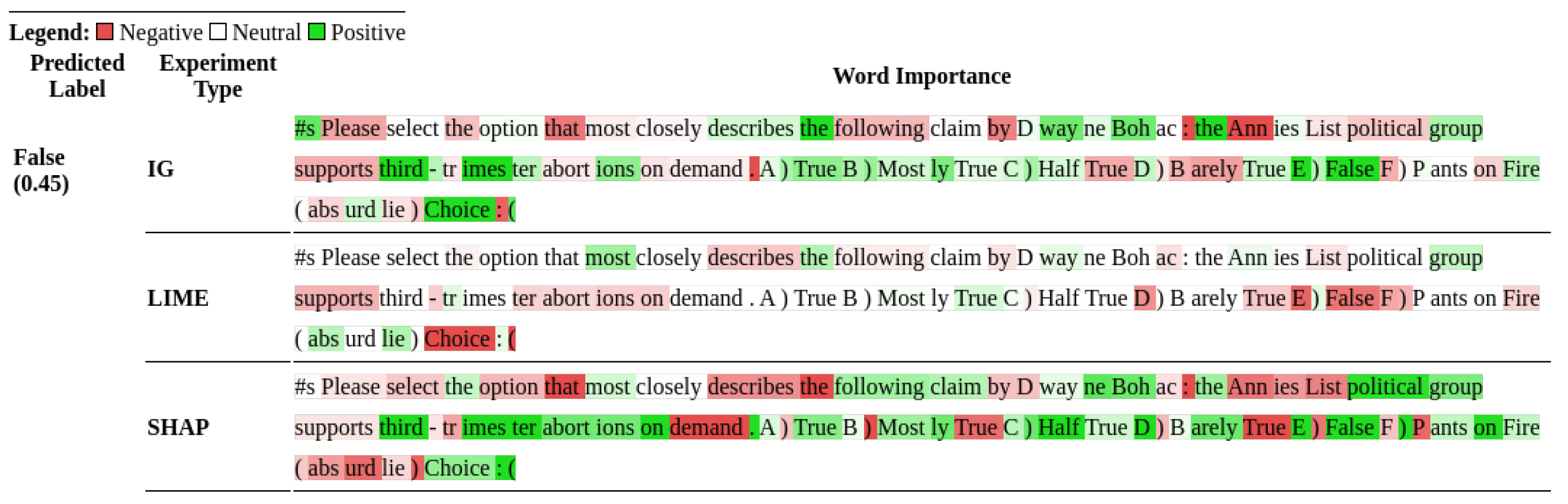
Despite these non-intuitive observations, LIME, SHAP, and Integrated Gradients do highlight features, which in this case are words or parts of words, in the prompt that humans would categorize as important. Hot topics, such as “third-trimester abortion” and “illegal aliens”, as well as large quantities, such as “billions” or “millions”, are often labeled as important features by at least one of the explainability methods, as seen in Figure 8, Figure 9, Figure 10 and Figure 11. The speaker and any named entities in the claim are also frequent contributors to model outputs. Similarly, strong actions or verbs within the claims, such as “murder”, are also labeled as important features (Figure 12). More of such information from the dataset is analyzed in Figure A2, Figure A3 and Figure A4 in Appendix A.

The results from the explainability methods do not entirely align with the quantitative results since they suggest that most of the models do focus on the correct aspects of prompts. In other words, these results suggest that LLMs understand the prompts and know what to focus on, but lack the correct knowledge, possibly because the LLMs were not trained on the corresponding facts.

The problem is further examined by analyzing differences in results between models. First, a comparison is made between numerical attribution values, which varied significantly amongst models. Figure 13 shows a summary of the comparison. Falcon showed the least average token-wise importance. This is likely because Falcon showed the lowest level of confidence in its predictions out of the four models that were compared. Confidence is indicated by the probabilities output from the softmax function when the model predicted the next token. It exhibited an average confidence of less than fifty percent for predicting the next token. This clarifies why Falcon has low token-wise importance when using explainability methods like SHAP and Integrated Gradients, whose attributions add up to the model’s prediction. Interestingly, the same trend holds for LIME attributions as well, as visible in Figure 13, even though the attributions are not additive. The opposite holds true as well. Models that were more confident in their results, such as Orca and Mistral, as seen in Figure 13, exhibited higher token-wise importance. Strangely, while Orca’s mean confidence is at least 20 percentage points less than Mistral’s, Orca’s mean LIME token-wise attribution is slightly greater than Mistral’s.

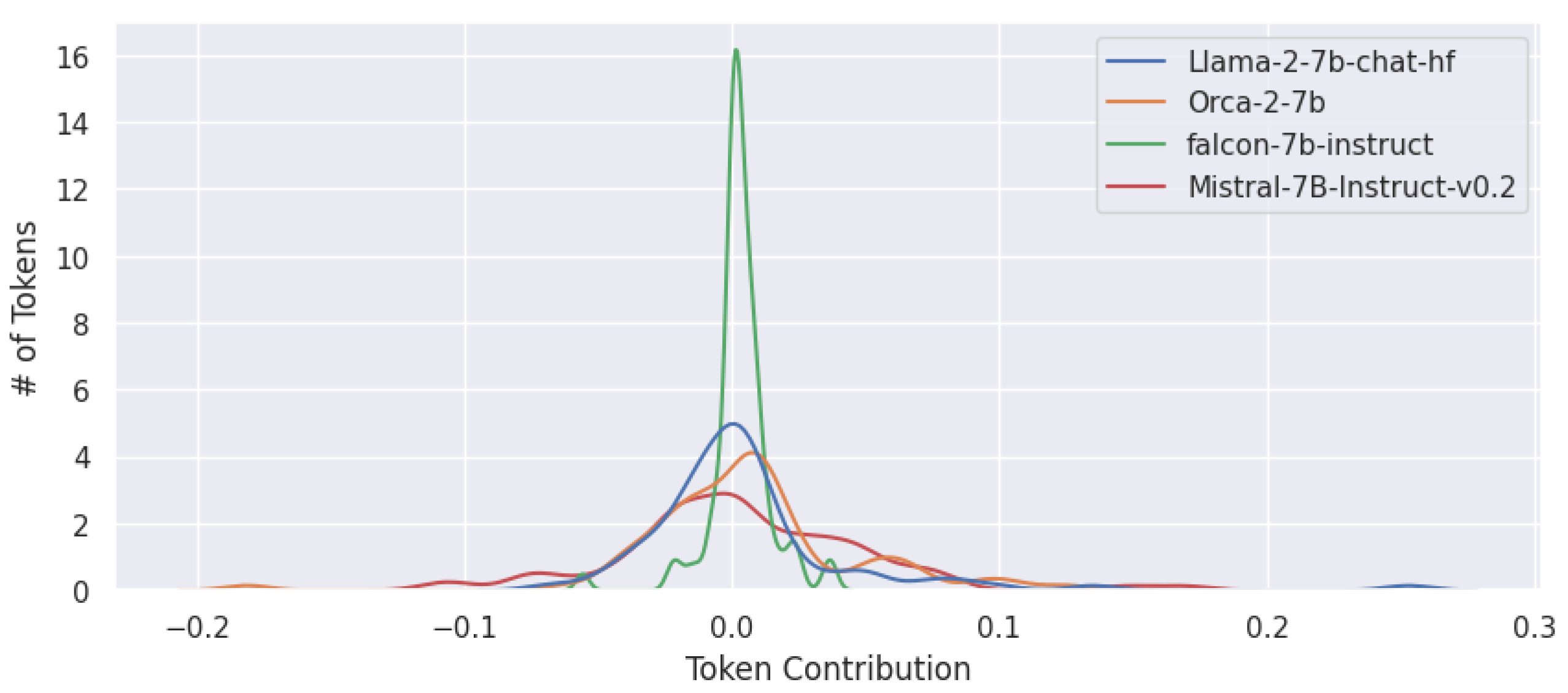
The distribution of the attributions plotted in Figure 14 shows that Falcon’s token-wise importance distribution is highly centered around 0 with a smaller standard deviation when compared to other models. In contrast, Mistral, which performed the best out of the models evaluated, has a different kind of plot. The curve in the plot reveals a token-wise significance distribution with more fluctuations, volatility, and a higher standard deviation. This may be a key factor, from an explainability perspective, why Mistral outperforms its competitors. The distributions in the plot suggest that Mistral prominently uses more tokens in the prompt than its competitors do, thereby allowing it to better respond to the prompt.

The initial plots used for comparisons were based on LIME, SHAP, and Integrated Gradients’ token-wise attributions. However, SHAP and Integrated Gradients attributions are additive and sum to the predicted probability. Therefore, the raw token-wise attributions may not be a fair comparison given the varying levels of confidence exhibited by different models. To account for this, each attribution is scaled by a factor of $\frac{1}{\mathrm{sum}\left(attribution\right)}$. The scaled graphs showed similar trends, as seen in Figure 15.

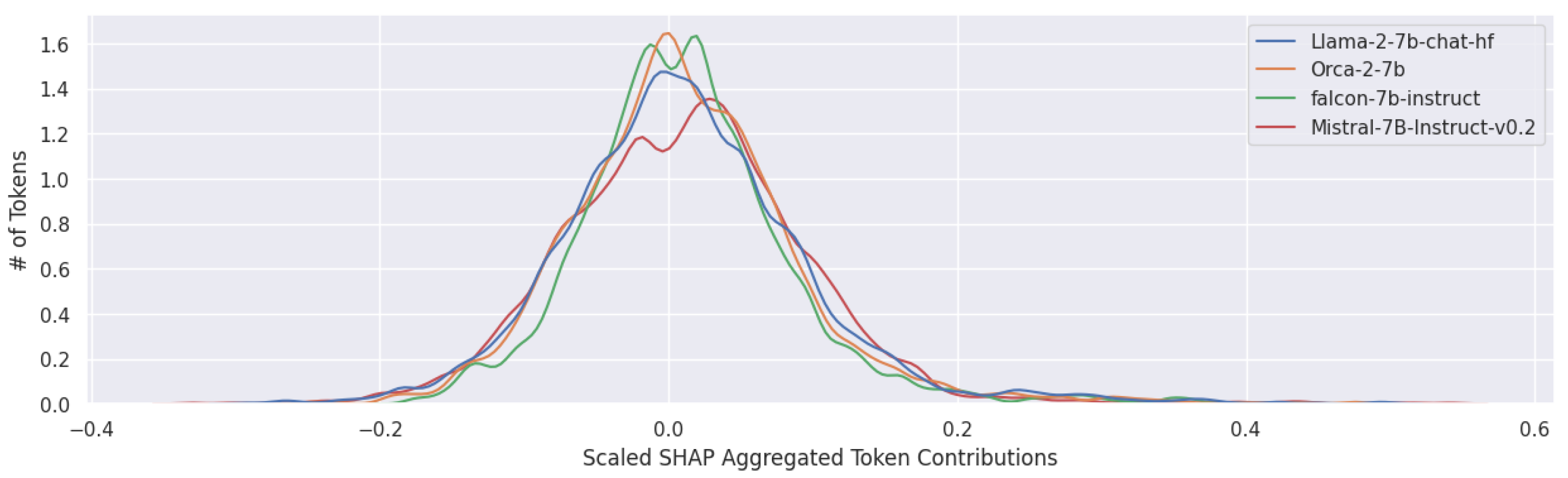
The plots reflect token-wise importance for specific entries within the LIAR dataset. The attributions produced by Integrated Gradients, LIME, and SHAP are all highly local. An aggregation of the attributions, despite losing information about local fluctuations, maintains most of the characteristics of the overall distributions. Accordingly, the aggregated scaled attributions are plotted in Figure 16. Notably, Falcon’s distribution curve still has the smallest standard deviation and the highest peak of all the models, confirming suspicions that Falcon does not pay enough attention to most of the tokens to answer prompts with the same accuracy as its peers. In contrast, models that perform better have wider distribution curves.

To determine how well models could explain their predictions, the next step was to compare the results from the explainability methods with explanations from the models themselves. When asked to explain their answers, models frequently pointed to background information regarding the topic and any named entities important to and appearing in the claim. Notably, while the speaker may be highlighted by explainability methods, models rarely cite information specific to the speaker. Perhaps more interestingly, models cited different evidence and provided different levels of detail when supporting their claims. Mistral and Orca’s explanations were on average longer and more detailed than their competitors. Moreover, Mistral and Orca often produced explanations without explicitly being prompted for them. Llama sometimes produced explanations without explicit prompting, and Falcon often required explicit prompting, at which point it would provide the shortest explanations, if any.

Nevertheless, side-by-side comparisons of model explanations (Figure 17) and current explainability algorithms appear to complement each other, as the latter reveals keywords in the text that appear to trigger the models’ world knowledge, which is revealed explicitly in the former. Once again, this suggests that models are capable of focusing on the right words and are only failing to answer correctly because they were trained on insufficient, outdated, or inaccurate information.

4. Discussion

The poor performance of several language models on the LIAR dataset was unexpected. The following paragraphs attempt to suggest conjectures to explain the reason for the models’ poor performance on the LIAR dataset.

One potential reason for the models’ poor performance is the data cutoff date. For LLMs, the data cutoff date is the date after which newer data are not incorporated into the training set. An older data cutoff date leads to outdated knowledge, which could negatively impact the models’ ability to detect misinformation. However, this conjecture is not the only reason. When the experiments were repeated with Google’s recently released Gemma 7b [27], Gemma’s accuracy on the LIAR dataset when evaluated on zero-shot prompts in bfloat16 precision was only 20%, which is roughly equivalent to the accuracies of the other models that were trained with older data cutoff dates.

Another possible conjecture is the difference in the datasets. This conjecture seems more likely than the previous one. When comparing LLM performance on LIAR with LLM performance on the datasets examined by Hu et al. [12] and also the COVID-19 dataset examined in this paper, the models severely underperform on LIAR than on other datasets. However, the datasets examined by Hu et. al [12], which are the Weibo 21 dataset [28] and the Gossip Cop dataset from FakeNewsNet [29], contain samples that are easily identified as information or misinformation by giveaways within the samples themselves, including emotionally charged words and differences in writing styles [12]. Most notably, Nan et al. [28] benchmarked their Weibo 21 dataset with Text CNNs, which achieved an average of over 80% accuracy, and Patwa et al. [6] benchmarked their COVID-19 dataset with SVMs, which outperformed other methods and achieved an average of over 90% accuracy. In contrast, CNNs, which outperformed SVMs on the LIAR dataset, achieved only an average of 27% accuracy on the LIAR dataset. This suggests that the LIAR dataset and the Weibo 21 dataset differ fundamentally in terms of the content of their samples. It also explains the differences in LLM accuracies on the different datasets; in both cases, zero to few-shot LLMs achieved accuracies in the same range as—although slightly less than—those of SLMs trained on the corresponding datasets. Similarly, the work conducted by Caramancion et al. [11] uses self-contained samples taken from social media posts that, like those from FakeNewsNet and Weibo 21, have giveaways within their structure that help LLMs achieve the high accuracy recorded in the paper.

This difference in datasets is interesting theoretically, as it suggests that something is missing in the LIAR dataset, preventing AI models, even LLMs trained on trillions of tokens, from accurately classifying samples based on the given labels. The missing aspect may be the context-specific background knowledge. The finer granularity of six labels versus two used for the classification may also be contributing to the poor performance. LLMs perform well at detecting COVID-19 misinformation, and COVID-19 information is something that LLMs have most likely seen a lot of. Future work may attempt to provide LLMs with the required context, perhaps by using Retrieval Augmented Generation (RAG) or fine-tuning, and assess their performance afterward.

Recent pushes for open-sourcing have led to many LLM companies open-sourcing their weights, and sometimes even open-sourcing the instruction datasets that they were fine-tuned on. Containing trillions of tokens and many terabytes of information, as opposed to the megabytes of tokens found in open-sourced assistant datasets, like OpenAssistant [30], these datasets comprise the majority of the data that models learn from and ultimately recite. Yet, despite trends toward open-sourcing, the datasets used to train these foundation models have not been open-sourced. For example, Touvron et al. [13] describe steps taken to clean, filter, and otherwise preprocess their training corpus. The authors do not reveal what their training corpus comprised. In another instance, Jiang et al. [15] only describe their model architecture but do not disclose the training corpus used for their model. There may be differences within the respective datasets used to train the models compared in this paper, leading to the differences in accuracies between models. There is also a chance that Reinforcement learning from Human Feedback (RLHF) to make models production-ready [31] may result in models being more adept at classifying certain types of misinformation, as the trainers working on RLHF may be more sensitive to certain types of misinformation. This may be another contributing factor to the immense differences in model accuracy on the COVID-19 dataset, especially given Mistral’s extensive guardrails. In future work, it may be interesting to use Mistral’s RLHF process on Llama models and evaluate whether they detect misinformation better afterward.

5. Conclusions

This work presented a quantitative and qualitative comparison of multiple large foundation models’ abilities to detect misinformation. This work also qualitatively inspected the relationship between LLM inputs and outputs to explain the differences in the models’ performance. In doing so, the limits of misinformation detection owing to the composition of datasets were compared. While LLMs alone are not currently capable of effective misinformation containment, augmented LLMs may eventually be part of an ecosystem of checks and cross-checks for misinformation containment. Future work may attempt to similarly benchmark larger models and verify that these trends hold even for larger models.

References

- Brown, T.B.; Mann, B.; Ryder, N.; Subbiah, M.; Kaplan, J.; Dhariwal, P.; Neelakantan, A.; Shyam, P.; Sastry, G.; Askell, A.; et al. Language Models are Few-Shot Learners. arXiv 2020, arXiv:2005.14165. [Google Scholar]
- Pendyala, V.; Kim, H. Assessing the Reliability of Machine Learning Models Applied to the Mental Health Domain Using Explainable AI. Electronics 2024, 13, 1025. [Google Scholar] [CrossRef]
- Pendyala, V.S. Misinformation Containment Using NLP and Machine Learning: Why the Problem Is Still Unsolved. In Deep Learning Research Applications for Natural Language Processing; IGI Global: Hershey, PA, USA, 2023; pp. 41–56. [Google Scholar]
- Pendyala, V.S.; Tabatabaii, F.S.A. Spectral analysis perspective of why misinformation containment is still an unsolved problem. In Proceedings of the 2023 IEEE Conference on Artificial Intelligence (CAI), Santa Clara, CA, USA, 5–6 June 2023; pp. 210–213. [Google Scholar]
- Wang, W.Y. “Liar, Liar Pants on Fire”: A New Benchmark Dataset for Fake News Detection. In Proceedings of the 55th Annual Meeting of the Association for Computational Linguistics (Volume 2: Short Papers), Vancouver, BC, Canada, 30 July–4 August 2017; pp. 422–426. [Google Scholar]
- Patwa, P.; Sharma, S.; Pykl, S.; Guptha, V.; Kumari, G.; Akhtar, M.S.; Ekbal, A.; Das, A.; Chakraborty, T. Fighting an Infodemic: COVID-19 Fake News Dataset. In Communications in Computer and Information Science; Springer International Publishing: Berlin/Heidelberg, Germany, 2021; pp. 21–29. [Google Scholar] [CrossRef]
- Das, S.D.; Basak, A.; Dutta, S. A Heuristic-driven Ensemble Framework for COVID-19 Fake News Detection. arXiv 2021, arXiv:2101.03545. [Google Scholar]
- Devlin, J.; Chang, M.W.; Lee, K.; Toutanova, K. BERT: Pre-training of Deep Bidirectional Transformers for Language Understanding. arXiv 2019, arXiv:1810.04805. [Google Scholar]
- Yang, Z.; Dai, Z.; Yang, Y.; Carbonell, J.; Salakhutdinov, R.; Le, Q.V. XLNet: Generalized Autoregressive Pretraining for Language Understanding. arXiv 2020, arXiv:1906.08237. [Google Scholar]
- Tonmoy, S.; Zaman, S.; Jain, V.; Rani, A.; Rawte, V.; Chadha, A.; Das, A. A comprehensive survey of hallucination mitigation techniques in large language models. arXiv 2024, arXiv:2401.01313. [Google Scholar]
- Caramancion, K.M. Harnessing the Power of ChatGPT to Decimate Mis/Disinformation: Using ChatGPT for Fake News Detection. In Proceedings of the 2023 IEEE World AI IoT Congress (AIIoT), Seattle, WA, USA, 7–10 June 2023; pp. 0042–0046. [Google Scholar] [CrossRef]
- Hu, B.; Sheng, Q.; Cao, J.; Shi, Y.; Li, Y.; Wang, D.; Qi, P. Bad Actor, Good Advisor: Exploring the Role of Large Language Models in Fake News Detection. arXiv 2024, arXiv:2309.12247. [Google Scholar] [CrossRef]
- Touvron, H.; Martin, L.; Stone, K.; Albert, P.; Almahairi, A.; Babaei, Y.; Bashlykov, N.; Batra, S.; Bhargava, P.; Bhosale, S.; et al. Llama 2: Open Foundation and Fine-Tuned Chat Models. arXiv 2023, arXiv:2307.09288. [Google Scholar]
- Almazrouei, E.; Alobeidli, H.; Alshamsi, A.; Cappelli, A.; Cojocaru, R.; Debbah, M.; Goffinet, É.; Hesslow, D.; Launay, J.; Malartic, Q.; et al. The Falcon Series of Open Language Models. arXiv 2023, arXiv:2311.16867. [Google Scholar]
- Jiang, A.Q.; Sablayrolles, A.; Mensch, A.; Bamford, C.; Chaplot, D.S.; de las Casas, D.; Bressand, F.; Lengyel, G.; Lample, G.; Saulnier, L.; et al. Mistral 7B. arXiv 2023, arXiv:2310.06825. [Google Scholar]
- Lin, S.; Hilton, J.; Evans, O. TruthfulQA: Measuring How Models Mimic Human Falsehoods. arXiv 2022, arXiv:2109.07958. [Google Scholar]
- Beeching, E.; Fourrier, C.; Habib, N.; Han, S.; Lambert, N.; Rajani, N.; Sanseviero, O.; Tunstall, L.; Wolf, T. Open LLM Leaderboard. 2023. Available online: https://huggingface.co/spaces/HuggingFaceH4/open_llm_leaderboard (accessed on 22 April 2024).
- Merrick, L. Randomized Ablation Feature Importance. arXiv 2019, arXiv:1910.00174. [Google Scholar]
- Ribeiro, M.T.; Singh, S.; Guestrin, C. “Why Should I Trust You?”: Explaining the Predictions of Any Classifier. arXiv 2016, arXiv:1602.04938. [Google Scholar]
- Sundararajan, M.; Taly, A.; Yan, Q. Axiomatic Attribution for Deep Networks. arXiv 2017, arXiv:1703.01365. [Google Scholar]
- Lundberg, S.; Lee, S.I. A Unified Approach to Interpreting Model Predictions. arXiv 2017, arXiv:1705.07874. [Google Scholar]
- Bills, S.; Cammarata, N.; Mossing, D.; Tillman, H.; Gao, L.; Goh, G.; Sutskever, I.; Leike, J.; Wu, J.; Saunders, W. Language Models Can Explain Neurons in Language Models. 2023. Available online: https://openaipublic.blob.core.windows.net/neuron-explainer/paper/index.html (accessed on 22 April 2024).
- Mukherjee, S.; Mitra, A.; Jawahar, G.; Agarwal, S.; Palangi, H.; Awadallah, A. Orca: Progressive Learning from Complex Explanation Traces of GPT-4. arXiv 2023, arXiv:2306.02707. [Google Scholar]
- Cohen, J. A coefficient of agreement for nominal scales. Educ. Psychol. Meas. 1960, 20, 37–46. [Google Scholar] [CrossRef]
- Chicco, D.; Jurman, G. The Matthews correlation coefficient (MCC) should replace the ROC AUC as the standard metric for assessing binary classification. Biodata Min. 2023, 16, 4. [Google Scholar] [CrossRef]
- Kokhlikyan, N.; Miglani, V.; Martin, M.; Wang, E.; Alsallakh, B.; Reynolds, J.; Melnikov, A.; Kliushkina, N.; Araya, C.; Yan, S.; et al. Captum: A unified and generic model interpretability library for PyTorch. arXiv 2020, arXiv:2009.07896. [Google Scholar]
- Mesnard, T.; Hardin, C.; Dadashi, R.; Bhupatiraju, S.; Sifre, L.; Rivière, M.; Kale, M.S.; Love, J.; Tafti, P.; Hussenot, L.; et al. Gemma. 2024. Available online: https://www.kaggle.com/models/google/gemma (accessed on 22 April 2024).
- Nan, Q.; Cao, J.; Zhu, Y.; Wang, Y.; Li, J. MDFEND: Multi-domain Fake News Detection. In Proceedings of the 30th ACM International Conference on Information & Knowledge Management, New York, NY, USA, 1–5 November 2021; pp. 3343–3347. [Google Scholar] [CrossRef]
- Shu, K.; Mahudeswaran, D.; Wang, S.; Lee, D.; Liu, H. FakeNewsNet: A Data Repository with News Content, Social Context and Dynamic Information for Studying Fake News on Social Media. arXiv 2018, arXiv:1809.01286. [Google Scholar] [CrossRef]
- Köpf, A.; Kilcher, Y.; von Rütte, D.; Anagnostidis, S.; Tam, Z.R.; Stevens, K.; Barhoum, A.; Duc, N.M.; Stanley, O.; Nagyfi, R.; et al. OpenAssistant Conversations—Democratizing Large Language Model Alignment. arXiv 2023, arXiv:2304.07327. [Google Scholar]
- Ouyang, L.; Wu, J.; Jiang, X.; Almeida, D.; Wainwright, C.L.; Mishkin, P.; Zhang, C.; Agarwal, S.; Slama, K.; Ray, A.; et al. Training language models to follow instructions with human feedback. arXiv 2022, arXiv:2203.02155. [Google Scholar]
Figure 1.
The approach used for answering the research questions.
Figure 2.
Zero-shot answer distribution for Falcon, Mistral, Llama, and Orca. A corresponds to True, B to Mostly True, C to Half True, D to Barely True, E to False, F to Pants on Fire, and UNK to an answer that fell into none of the above categories. Falcon’s answers are highly skewed toward B (Mostly True). Mistral exhibited the most diverse answer distribution, which may be why it was more accurate than other models. Llama’s answers are highly skewed toward B (Mostly True) and D (Barely True). Orca is highly biased toward A (True).
Figure 3.
Models’ deterministic 0-shot answer distribution for LIAR with binary truth values. While we expected the distributions to look much closer to a uniform distribution, the models continue to produce skewed distributions. Orca’s distribution continues to be skewed toward A (True), while Llama’s distribution is skewed toward B (False). While Falcon’s normal 0-shot distribution is skewed toward Mostly True, its binary distribution is skewed toward B (False). Some of the answers are neither A nor B, so are categorized as UNK.
Figure 4.
Explainability results from Integrated Gradients, LIME, and SHAP for Falcon LLM on a sample from the LIAR dataset.
Figure 5.
Explainability results from Integrated Gradients, LIME, and SHAP for Orca LLM on a sample from the LIAR dataset.
Figure 6.
Explainability results from Integrated Gradients, LIME, and SHAP for the Mistral LLM on a sample from the LIAR dataset.
Figure 7.
Explainability results from Integrated Gradients, LIME, and SHAP for the Llama LLM on a sample from the LIAR dataset.
Figure 8.
Explainability results from Integrated Gradients, LIME, and SHAP for the Mistral LLM on a sample from the LIAR dataset showing how important the hot topic of “federal military spending” is for the LLM’s prediction.
Figure 9.
Explainability results from Integrated Gradients, LIME, and SHAP for the Mistral LLM on a sample from the LIAR dataset showing how important the hot topic of “illegal aliens” is for the LLM’s prediction.
Figure 10.
Explainability results from Integrated Gradients, LIME, and SHAP for the Llama LLM on a sample from the LIAR dataset showing the importance of large quantities, like “millions” on the LLM’s prediction.
Figure 11.
Explainability results for Mistral LLM showing the importance of controversial issues such as “third-trimester abortion”.
Figure 12.
Explainability results for Mistral LLM showing the importance of words that hint at controversial associations, such as “percent”, “murders”, and “illegal aliens”.
Figure 13.
Mean confidence and LIME mean attributions. Mistral’s mean confidence was the highest, which explains why its token-wise Integrated Gradients and SHAP attribution scores were the greatest. The converse applies to Falcon. Notably, the relative distribution of LIME token-wise attribution scores roughly matches that of the model confidences.
Figure 14.
Integrated Gradients distributions pre-scaling on a random sample from the LIAR dataset. Falcon’s distribution is highly centered around 0, while other models exhibit wider distributions.
Figure 15.
Distributions from the Integrated Gradients after scaling on the same random sample from the LIAR dataset. Even after accounting for scaling differences, Falcon’s distribution still has the tallest peak out of the models we compared, suggesting that most tokens do not impact Falcon’s output.
Figure 16.
Aggregated scaled Integrated Gradients attributions, aggregated LIME attributions, and aggregated scaled SHAP attributions. On the given subset of the dataset examined, the explainability methods revealed that Falcon consistently ignores many tokens compared to its competitors, potentially leading to its poor performance. All the explainability methods reveal that Falcon’s distribution curve is the least wide, although it is much clearer from LIME and Integrated Gradients than it is from SHAP.
Figure 17.
LIME outputs and LLaMa explanations. LLaMa cites background evidence related to the topics and words that LIME highlighted, suggesting that the models understand the prompts but may fail to respond correctly due to incorrect or outdated background knowledge.