
ML-Based Software Defect Prediction in Embedded Software for Telecommunication Systems (Focusing on the Case of SAMSUNG ELECTRONICS)

1
Software Engineering Team, Samsung Electronics Co. Ltd., Suwon 16677, Republic of Korea
2
Division of Computer Engineering, The Cyber University of Korea, Seoul 02708, Republic of Korea
*
Author to whom correspondence should be addressed.
Electronics 2024, 13(9), 1690; https://doi.org/10.3390/electronics13091690
Submission received: 10 March 2024
/
Revised: 15 April 2024
/
Accepted: 22 April 2024
/
Published: 26 April 2024
(This article belongs to the Special Issue Software Analysis, Quality, and Security)
Abstract
:Software stands out as one of the most rapidly evolving technologies in the present era, characterized by its swift expansion in both scale and complexity, which leads to challenges in quality assurance. Software defect prediction (SDP) has emerged as a methodology crafted to anticipate undiscovered defects, leveraging known defect data from existing codes. This methodology serves to facilitate software quality management, thereby ensuring overall product quality. The methodologies of machine learning (ML) and one of its branches, deep learning (DL), exhibit superior accuracy and adaptability compared to traditional statistical approaches, catalyzing active research in this domain. However, it makes it hard to generalize, not only because of the disparity between open-source projects and commercial projects but also due to the differences in each industrial sector. Consequently, further research utilizing datasets sourced from diverse real-world sectors has become imperative to bolster the applicability of these findings. For this study, we utilized embedded software for use with the telecommunication systems of Samsung Electronics, supplemented by the introduction of nine novel features to train the model, and a subsequent analysis of the results ensued. The experimental outcomes revealed that the F-measurement metric has been enhanced from 0.58 to 0.63 upon integration of the new features, thereby signifying a performance augmentation of 8.62%. This case study is anticipated to contribute to bolstering the application of SDP methodologies within analogous industrial sectors.
1. Introduction
In the present era, software represents one of the most rapidly evolving domains. Companies are leveraging software as a core component for enhancing productivity, reducing costs, and exploring new markets. Today’s software is providing more functionality, processing bigger datasets, and executing more complex algorithms compared to those in the past. Furthermore, the software must interact with increasingly intricate external environments and must satisfy diverse constraints. Consequently, the scale and complexity of software exhibit swift escalation. Measurement data at Volvo showed that a Volvo vehicle in 2020 had about 100 million LOC. This means that the vehicle had software equivalent to 6000 average books, which can be equivalent to a decent town library [1].
As the scope and intricacy of software expand, ensuring its reliability becomes an increasingly formidable task [2]. It is practically unachievable to detect and remediate all defects within a given finite time and with limited resources. Software defects refer to “errors or failures in software”, which could result in inaccurate or unintended behavior and the triggering of unforeseen behavior [3,4]. Quality management and testing expenditures aimed at guaranteeing reliability constitute a substantial portion of overall software development costs. This expense escalates exponentially to rectify software defects in the later stages of development [5]. Hence, utilizing the available resources and minimizing defects in the initial phase of software development are crucial to obtaining high-quality outcomes [6]. Such measures can curtail the expenses associated with defect rectification and mitigate the adverse ramifications of defects.
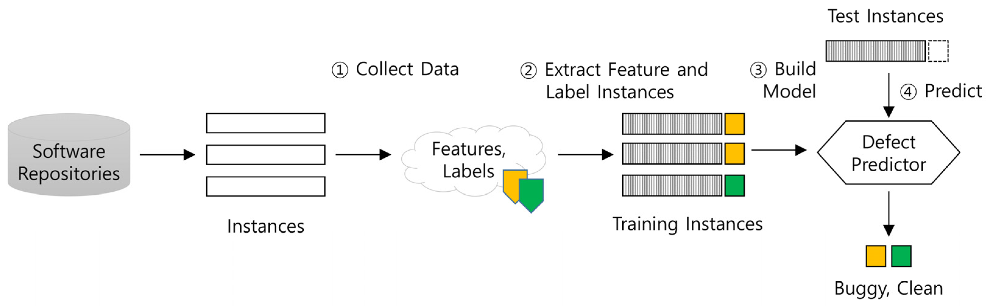
Software defect prediction (SDP) is a technique geared toward identifying flawed modules within source code, playing a crucial role in ensuring software quality [7,8]. SDP not only bolsters software quality but also economizes on time and cost by efficiently allocation resources to areas with a high probability of defects under limited time and resource situation. Additionally, SDP augments testing efficiency by facilitating the identification of critical test cases and optimizing the test sets effectively [9]. Machine learning-based software defect prediction (ML-SDP or SDP) represents a technological framework that leverages attributes gleaned from historical software defect data, software update records, and software metrics to train machine learning models for defect prediction [8]. M. K. Thota et al. [8] envision that ML-SDP will engender more sophisticated and automated defect detection mechanisms, which are emerging as focal points of research within the realm of software engineering. Figure 1 elucidates the foundational process of SDP. The process includes collecting data (①), extracting the features and labeling them (②), training and testing the models (③), and operationalizing the defect predictor for real-world application (④).
Nonetheless, the applicability of SDP models derived from previous research may encounter limitations when we directly transpose them to industrial sectors. Disparities in software attributes and the root causes of defects are apparent across various industry sectors, and even within a single industrial sector. Discrepancies in software development methodologies and practices among projects can engender variations in software attributes and the causes of defects. However, accessing real industrial sector data is often challenging as the data are either not publicly available or are difficult to obtain, making research challenging regarding such data [10]. Stradowski et al. [11] underscore that although machine learning research aimed at predicting software defects is increasingly valid in industrial settings, there is still a lack of sufficient practical focus on bridging the gap between industrial requirements and academic research, which could help narrow the gap between them. Practical impediments, including disparities in software attributes, constraints in metric measurement, data scarcity, and inadequate cost-effectiveness may impede the application of SDP methodologies from academic research to industrial sectors. Hence, we can facilitate the harnessing of SDP methodologies and foster future research initiatives by suggesting the practical applicability, implementation, and deployment of SDP through empirical case studies within industrial sectors.
In this research, we have endeavored to devise an SDP model by leveraging data sourced from embedded software utilized in Samsung’s telecommunication systems. To tailor the SDP model to the specific nuances of embedded software for telecommunication systems, we have introduced nine novel features. These features encompass six software quality metrics and three source code type indicators. Harnessing these features, we have trained a machine learning model to formulate the SDP model and scrutinized the impact of the new features on predictive efficacy to validate their effectiveness. The experimental outcomes revealed that the SDP model incorporating the nine new features exhibited a notable enhancement of 0.05 in both Recall and F-measurement metrics. Moreover, the overall predictive performance of the SDP model was characterized by an accuracy of 0.8, precision of 0.55, recall of 0.74, and an F-measurement of 0.63. This performance level is comparable to the average accuracy achieved across 11 projects, as discussed by Kamei et al. [12]. The results of this study confirm the contribution of the nine new features to predictive performance. Moreover, by examining the predictive contributions of each software quality metric, we can identify meaningful indicators for software quality management. Additionally, providing source codes to the machine learning model resulted in enhanced predictive capability. These findings suggest that SDP can be utilized for the early detection of software defects, efficient utilization of testing resources, and evaluation of the usefulness of software quality metrics in similar domains.
This paper adheres to the following structure: Section 2 explores the theoretical foundations of software defect prediction (SDP), reviews the prior research in the field, and elucidates the limitations of previous studies. Section 3 encompasses an in-depth analysis of the characteristics of embedded software data pertinent to telecommunication systems, outlines the research questions, and delineates the experimental methodology employed. Section 4 scrutinizes the experimental findings and extrapolates conclusions pertaining to the research questions posited. Lastly, Section 5 expounds upon the implications and constraints of this study, alongside outlining avenues for future research endeavors.
2. Related Work
2.1. Software Defect Prediction Applied in Open-Source Projects
The methodologies of machine learning (ML) and one of its branches, deep learning (DL), exhibit heightened accuracy and versatility in comparison to traditional statistical approaches, thus catalyzing active research endeavors [13,14,15,16].
Khan et al. [17] employed Bayesian belief networks, neural networks, fuzzy logic, support vector machines, expectation maximum likelihood algorithms, and case-based reasoning for software defect prediction, offering insights into the strengths, weaknesses, and prediction accuracy of each model. Their research outcomes furnish valuable guidance in selecting appropriate methodologies tailored to available resources and desired quality standards. The spectrum of research on SDP encompasses diverse techniques such as preprocessing, mitigating class imbalance, optimal feature selection [18,19], the adoption of novel machine learning algorithms [20,21,22], and hyperparameter optimization to augment prediction performance.
Predictive performance exhibits wide-ranging variability, with F-measurement criteria spanning from 0.50 to 0.99. Given the pronounced divergence in performance observed across studies in the literature, generalizing the findings of individual investigations proves challenging. Table 1 encapsulates a summary of previous research endeavors pertaining to SDP applied in open-source projects.
Shafiq et al. [5] introduced the ACO-SVM model, which amalgamates the ant colony optimization (ACO) technique with the support vector machine (SVM) model. ACO serves as an optimization technique for feature selection. In their investigation, conducted utilizing the PC1 dataset, the ACO-SVM model showcased a specificity of 98%. This performance surpassed SVM by 5%, KNN by 4%, and the naive Bayes (NB) classifier by 8%.
Malhotra and Jain [23] undertook defect prediction by focusing on the open-source software Apache POI. They leveraged object-oriented CK metrics [30] and the QMOOD (quality model for object-oriented design) as features and juxtaposed various classification models, including linear regression, random forest, Adaboost, bagging, multilayer perceptron, and a support vector machine. Performance assessments based on metrics such as the area under the ROC curve (AUC-ROC), sensitivity, specificity, precision, and accuracy indicated that the random forest and bagging results surpassed other models in predictive efficacy.
Lee et al. [25] proposed a method for SDP that utilizes source code converted into images instead of software metrics. In their study, conducted using publicly available data from the PROMISE repository, they found that classifying keywords, spaces, and newline characters within the source code and converting them into images contributed to performance improvement.
Kim et al. [26] introduced a defect prediction model based on the state-of-the-art deep learning technique Ft-Transformer (feature tokenizer + Transformer). This model conducted experiments using LOC (line of code) and software complexity metrics as features for targeting open-source projects. It was observed that this model exhibited superior performance compared to XGBoost and CatBoost.
Choi et al. [27] applied a generative adversarial network (GAN), an adversarial neural network model, to tackle the class imbalance issue in SDP. Their experimentation, focusing on open-source projects and employing line of code (LOC) and software complexity metrics as features, demonstrated an enhancement in performance through the utilization of the GAN model to address the class imbalance.
Lee et al. [28] employed TabNet, a tabular network, for SDP, comparing its efficacy against XGBoost (XGB), random forest (RF), and a convolutional neural network (CNN). The study utilized LOC and software complexity metrics as features, targeting publicly available data from the PROMISE repository and employing SMOTE as a preprocessing technique. The findings revealed TabNet’s superior performance, achieving a recall performance of 0.85 in contrast to 0.60 for XGBoost.
Qihang Zhang et al. [29] conducted SDP research employing the Transformer architecture. By leveraging Transformer, the predictive performance based on F-measurement demonstrated an improvement of 8% compared to CNN. This investigation encompassed nine open-source projects, achieving an average F-measurement prediction performance of 0.626.
Indeed, the studies mentioned primarily concentrated on open-source projects, potentially overlooking the diverse software characteristics prevalent in real industrial domains, which can significantly impact defect occurrence [11]. Projects within real industrial domains are managed according to considerations such as budgetary constraints, project schedules, and resource allocation while adhering to national policies and standard specifications. Consequently, disparities in software attributes and defect patterns between open-source and industrial domain projects may arise. Hence, further research endeavors leveraging datasets sourced from various real industrial domains are imperative to ensure the generalizability of findings and enhance the applicability of defect prediction methodologies across diverse software development landscapes.
2.2. Software Defect Prediction Applied in Real Industrial Domains
Case studies of software defect prediction techniques applied in real industrial domains consistently demonstrate the applicability and utility of machine learning-based software defect prediction technologies in industrial sectors. However, when applied in real industrial settings, factors such as organization- and domain-specific software, as well as differences in development processes and practices, can influence the available data and predictive capabilities. Additionally, the prediction performance shows significant variability across studies, indicating the difficulty of extrapolating specific research findings to other domains. Stradowski et al. [11] suggest that while machine learning research on software defect prediction is increasingly being validated in industry, there is still a lack of sufficient practical focus to bridge the gap between industrial requirements and academic research. Table 2 presents previous studies on software defect prediction that has been applied in real industrial domains.
Xing et al. [31] proposed a method for predicting software quality utilizing a transductive support vector machine (TSVM). Their experimentation focused on medical imaging system (MIS) software, comprising 40,000 lines of code. The feature set encompassed 11 software complexity metrics, including change reports (CRs) and McCabe’s cyclomatic complexity [36]. The study yielded a Type II error rate of 5.1% and a classification correct rate (CCR, accuracy) of 0.90. SVM demonstrated robust generalization capabilities in high-dimensional spaces, even with limited training samples, facilitating rapid model construction.
Tosun et al. [32] undertook SDP within the GSM project of the Turkish telecommunications industry. They opted for the naïve Bayes classification model due to its simplicity, robustness, and high prediction accuracy. Confronted with a dearth of sufficient and accurate defect history information, they conducted transfer learning utilizing data from NASA projects. This study underscores the feasibility and effectiveness of applying machine learning to software defect prediction within real industrial domains, despite the inherent challenges.
Kim et al. [33] introduced the REMI (risk evaluation method for interface testing) model tailored for SDP concerning application programming interfaces (APIs). Their experiments utilized datasets sourced from Samsung Tizen APIs, incorporating 28 code metrics and 12 process metrics. The model opted for the random forest (RF) method due to its superior performance compared to alternative models.
Kim et al. [34] applied software defect prediction techniques within the automotive industry domain. The research entailed experiments conducted on industrial steering system software, employing a combination of software metrics and engineering metrics. Eight machine learning models were compared, including linear regression (LR), K-nearest neighbor (KNN), a support vector machine (SVM), decision tree (DT), multi-layer perceptron (MLP), and random forest (RF), among others. Notably, RF emerged as the top performer, achieving a ROC-AUC of 92.31%.
Kang et al. [35] implemented SDP within the maritime industry domain. Their approach involved addressing data imbalances using a synthetic minority oversampling technique (SMOTE) and incorporating 14 change-level metrics as software metrics. The experimental outcomes revealed exceptional software defect prediction performance, with an accuracy of 0.91 and an F-measure of 0.831. Furthermore, the study identified that the crucial features influencing prediction varied from those observed in other industry domains, underscoring the influence of organizational practices and domain-specific conventions.
In this study, we leverage data sourced from Samsung’s embedded software designed for telecommunication systems. This dataset comprises nine distinct features, encompassing six metrics that are indicative of software quality and three attributes delineating the source file types. Additionally, we meticulously assess the influence of these features on prediction performance to validate the efficacy of the newly introduced attributes.
3. Materials and Methods
3.1. Research Questions
In this study, we formulate the following four research questions (RQs):
RQ1.
How effectively does the software defect prediction (SDP) model anticipate defects?
Utilizing performance evaluation metrics such as accuracy, precision, recall, F-measurement, and the ROC-AUC score, the performance of the SDP with embedded software for telecommunication systems is compared with prior research findings.
RQ2.
Did the incorporation of new features augment the performance of SDP?
Through a comparative analysis of performance before and after the integration of previously utilized features and novel features, and by leveraging the Shapley value to assess the contribution of new features, the significance of software quality indicators and source file type information is evaluated.
RQ3.
How accurately does the SDP model forecast defects across different versions?
The predictive efficacy within the same version of the dataset, when randomly partitioned into training and testing subsets, is contrasted with predictive performance across distinct versions of the dataset that are utilized for training and testing. This investigation seeks to discern variances in defect prediction performance when the model is trained on historical versions with defect data and is tested with predicting defects in new versions.
RQ4.
Does predictive performance differ when segregating source files by type?
Software developers and organizational characteristics are important factors to consider in software defect research. F. Huang et al. [37] analyzed software defects in 29 companies related to the Chinese aviation industry and found that individual cognitive failures accounted for 87% of defects. This suggests that individual characteristics and environmental factors may significantly impact defect occurrence. In the current study source files are grouped based on software structure and software development organization structure, and the predictive performance is compared between cases where the training and prediction data are in the same group and cases where they are in different groups. This aims to ascertain the impact of source file type information on prediction accuracy.
3.2. Dataset
In this study, data originating from the base station software development at Samsung were utilized.
A base station serves as a wireless communication infrastructure, facilitating the connection between user equipment (UE) and the core network, thereby enabling wireless communication services. The base station software, deployed within the base station, assumes responsibility for controlling the hardware of the base station and facilitating communication between mobile users and the base station itself. Its functionalities encompass signal processing, channel coding, scheduling, radio resource management, and handover and security protocols. Figure 2 elucidates the structure of the base station software, illustrating the mapping relationship between the components of the base station software and the specifications outlined in the Third-generation Partnership Project technical specification (3GPP TS) 38.401 [38].
The base station software undergoes the continuous development of new versions. The development of 5G base station software according to the 3GPP 5G roadmap commenced around 2020 or earlier, with two or more packages being developed and deployed annually. Prior to the introduction of 5G mobile communication services, there existed 4G mobile communication services. Therefore, the development of 5G base station software involved extending the functionality of 4G base station software to also support 5G services. Consequently, if we consider the inclusion of 4G base station software, the development of base station software dates back to before 2010, indicating over 10 years of continuous development and the deployment of new features.
The requirements for base station software are influenced by various factors. Figure 3 illustrates how these requirements are incorporated into new versions of the base station software.
The first set of requirements originates from international standardization organizations such as ITU-T, 3GPP, and IEEE. These organizations continually enhance the existing standards and introduce new ones to align with advancements in wireless communication technology, thereby necessitating the development of base station software to accommodate these evolving specifications. The second set of requirements emerges from the customers of base station systems, including network operators and service providers. These entities consistently pursue novel service development and service differentiation strategies to maintain a competitive advantage in the market. The requirements stemming from these endeavors drive the development of base station software to meet the evolving demands of customers. Lastly, internal demands within base station manufacturers contribute to requirement generation. In order to sustain a competitive edge in the market, base station manufacturers continuously innovate by developing new hardware products and introducing features that differentiate them from those of other manufacturers.
The requirements arising from these three sources are translated into features of the base station and are subsequently incorporated into the base station software. These additional base station features are then included in future base station software packages for deployment, ultimately facilitating the delivery of services to end-users, namely, mobile subscribers, through their deployment on operational base stations.
The base station software exhibits several characteristics. Firstly, due to the continuous development of new versions over a period of more than 20 years, the existing code undergoes expansion and branching, leading to increased complexity and a higher likelihood of duplicate code. Secondly, the differentiation demands made by various customers result in multiple branches in the codebase, contributing to increased complexity and making code maintenance challenging. Thirdly, there is the continuous development of new hardware models. The base station software is continuously expanded to support new hardware products, leading to increased code complexity to accommodate various models and address non-functional requirements such as real-time processing and memory optimization. This complexity results in features such as increased code complexity to support diverse models, preprocessing to reduce runtime image size, and the use of common memory to minimize data copying [39,40,41,42,43]. Lastly, there are heterogeneous characteristics among the subsystems and blocks of these software systems. The subcomponents of these systems possess unique software characteristics due to differences in the technical domains; these are developed by personnel with expertise in each technical domain. Examples of these technical domains include wireless communication technology, call processing, traffic processing, network management, and operating system and middleware technology.
In this study, three versions of base station software developed between 2021 and 2022 serve as the experimental dataset. The cumulative number of sample files across the three versions amounts to 17,727, with 3993 instances (22.5%) exhibiting defects, labeled as “buggy files” within their respective versions (see Table 3). Notably, there do exist variations in both the number of samples and the buggy rate across the different versions. The codebase comprises a blend of C and C++ languages, with C constituting 60.7% and C++ encompassing 39.3% of the total codebase (see Table 4). Additionally, the sample rate denotes the proportion of files that were either newly created or modified relative to the total files, spanning a range from 40% to 74%. The submitter count signifies the number of individuals involved in coding, ranging from 897 to 1159 individuals. Furthermore, the feature count denotes the tally of added or modified base station features, with 353, 642, and 568 features integrated in Versions 1, 2, and 3, respectively. The development period for each package is either 3 or 6 months.
3.3. Research Design
The experiments for developing the SDP model are organized into six distinct steps, with each delineated to accomplish specific objectives. Figure 4 provides an overview of the scope encompassed by each step within the experiment.
In the first data collection step (①), the recent data from the development projects of the base station software, encompassing the latest three versions, are gathered to be utilized as experimental data. The second data processing step (②) involves various tasks such as outlier correction based on quartiles, oversampling to resolve class imbalances, scaling for uniformity in the feature value ranges, appropriate feature selection for model construction, and data selection suitable for model building. In the third data-splitting step (③), the training and testing data are divided using random splitting, version-based splitting, and specific group-based splitting methods. Version-based splitting is utilized for cross-version prediction, while group-based splitting is employed for experiments involving cross-group prediction. The fourth step (④) involves model selection, where machine learning algorithms like LR (linear regression), XGB (XGBoost), RB (random forest), and MLP are employed, after which the model with the highest prediction performance is chosen. In the fifth step (⑤), model evaluation is conducted using metrics such as accuracy, precision, recall, F-measurement, and the ROC-AUC score. Finally, in the sixth step (⑥) of the model analysis, feature importance and the Shapley value are utilized to analyze the significance of features.
Figure 5 delineates the process of gathering training data and executing defect prediction in a scenario characterized by the continuous development of new software versions. Feature data and the defect data acquired from version N serve as the training dataset for the machine learning model. Subsequently, the trained model is applied to predict defects using the feature data collected from version N + 1.
In the design/implementation phase, both the introduction and the removal of defects occur simultaneously. During this phase, defects are addressed through methods such as code reviews, unit testing, and other quality assurance practices. Ideally, all defects introduced during the design/implementation phase should be removed before the verification/maintenance phase. Defects that are not addressed during the design/implementation phase are detected during the verification/maintenance phase. Machine learning is then employed to learn the characteristics of modules containing these defects. In the design/implementation phase of version N + 1, software defect prediction (SDP) is used to identify modules similar to those in version N that experienced defects, categorizing them as likely to be buggy modules with similar characteristics.
3.4. Software Metrics
Software metrics quantify the characteristics of software into objective numerical values and are classified into project metrics, product metrics, and process metrics [44]. In this study, product metrics and process metrics are utilized as features for machine learning training. Product metrics pertain to metrics related to product quality assessment and tracking. Representative examples of product metrics include code complexity and the number of lines of code. Process metrics, on the other hand, relate to process performance and analysis. Examples of process metrics accumulated during the development process include the code change volume, code commit count, and number of coding personnel. Raw data collected from software quality measurement systems consist of metrics at both the function and file levels, necessitating the transformation of function-level metrics into file-level metrics. The “min/max/sum” marked in the “Comments” field of Table 5 indicates the conversion of function-level metrics to the corresponding file-level metrics. Additionally, identifiers such as the subsystem identifier, block identifier, and language identifier are employed to differentiate between file types. Subsystems represent the subcomponents of software systems, while blocks are the subcomponents of subsystems.
In this study, the selection of features was guided by established metrics validated in prior research, aligning with Samsung’s software quality management policy, which encompasses quality indicators and source file type information. Given the amalgamation of C and C++ programming languages within the codebase, we considered metrics that are applicable to both languages. Our feature set encompassed foundational software metrics such as code size, code churn, and code complexity, complemented by additional metrics specified by Samsung’s software quality indicators to bolster prediction efficacy. Additionally, we extracted subsystem and block information, representing the software’s hierarchical structure, from the file path information. To account for the mixed presence of C and C++ files, we also incorporated identifiers to distinguish between them. The newly introduced metrics in this research are highlighted in gray in Table 5 below.
Metrics derived from Samsung’s software quality indicators include the GV (global variable), MCD (module circular dependency), DC (duplicate code), and PPLOC (Preprocessor LOC). These metrics were derived by analyzing the defects identified during system testing by the software validation department. Figure 6 illustrates the process of measuring metrics in the software development process and improving metrics based on defect prevention. The software quality management system periodically measures quality metrics, including the metrics related to code. When defects are detected during system testing, an analysis of these defects is conducted, leading to the derivation of metrics for proactive defect detection. These metrics are then added back into the software quality management system’s quality indicators and are measured regularly.
In industrial software development projects, domain-specific metrics are frequently utilized to bolster prediction accuracy. Many of these metrics were omitted from this study due to disparities in development methodologies or insufficient data accumulation. For instance, metrics such as EXP (developer experience), REXT (recent developer experience), and SEXP (developer experience on a subsystem), as employed by Kamei et al. [12], were not integrated into our research. Instead, to better align with the attributes of embedded software for telecommunication systems, we introduced nine supplementary features, as delineated below.
- The GV (global variable) represents a count of the global variables in each file that reference variables in other files. Global variables increase the dependencies between modules, deteriorating maintainability and making it difficult to predict when and by which module a value is changed, thereby complicating debugging. Therefore, it is generally recommended to use global variables at a moderate level to minimize the risk of such issues. However, in embedded software, there is a tendency toward the increased usage of global variables due to constraints in speed and memory.
- MCD (module circular dependency) indicates the number of loops formed when connecting files with dependencies. Having loops deteriorates the maintainability of the code, so it is recommended to avoid creating loops. In the case of large-scale software development, such as communication system software, where multiple developers work on the code for extended periods, such dependencies can unintentionally arise.
- DC (duplicate code) represents the size of the repetitive code. When there is a lot of duplicate code, there is a higher risk of missing modifications to some of the code during the maintenance process, which can be problematic. Therefore, removing duplicate code is recommended. Embedded software for communication systems tends to have a large overall codebase, where the code continuously expands to support new hardware developments. At the same time, development schedules may not allow sufficient time for the timely market release of new versions, and there is less likelihood of the same developer consistently handling the same code. In such environments, developers may not have enough time to analyze the existing code thoroughly, leading them to copy the existing code when developing code for new hardware models, resulting in duplicates.
- PPLOC (Preprocessor LOC) is the size of the code within preprocessor directives such as #ifdef… and #if… These codes are assessed for compilation inclusion based on the satisfaction of conditions written alongside preprocessor directives during the compilation time. In embedded software for communication systems, due to the memory constraints of hardware devices like DSPs (digital signal processors), the only codes running on each piece of hardware are included in the execution image to minimize code size. For this purpose, preprocessor directives are employed. However, similar to DC, this practice leads to the generation of repetitive, similar codes, increasing the risk of omitting modifications to some codes during code editing.
- cov_l and cov_b, respectively, represent line coverage and branch coverage, indicating the proportion of tested code out of the total code. A lower proportion of tested code in developer testing increases the likelihood of defects being discovered during system testing.
- Critical/Major denotes the number of defects detected by static analysis tools. If these defects are not addressed by the developer in the testing phase, the likelihood of defects being discovered during system testing increases.
- FileType serves as an identifier for distinguishing between C code and C++ code. It is a feature aimed at incorporating the differences between C and C++ code into machine learning training.
- Group_SSYS serves as information to identify subsystems. Subsystems are subunits that constitute the entire software structure. This feature enables the machine learning model to reflect the differences between subsystems in its training.
- Group_BLK serves as information to identify blocks. Blocks are subunits that constitute subsystems in the software structure. This feature enables the machine learning model to reflect the differences between blocks in its training.
3.5. Defect Labeling
The defect labels are determined based on the defect information described in the code commit description. In reality, it is challenging to manage defect information in a way that enables the perfect tracking of defect codes in industrial domains. Defect tracking requires additional effort, but it is often difficult to allocate resources for this purpose. Therefore, it is necessary to find an optimal solution tailored to the specific development processes and practices of each domain or organization. In this study, code commit descriptions were subjected to text mining to classify code commits containing topics that are highly relevant to the defects as code commits resulting from defect fixes.
3.6. Mitigating Class Imbalance
The data used in this study contain class imbalance, with the buggy class accounting for 22.5% of the data. This imbalance arises because the proportion of actual buggy code in the entire source code is significantly lower than that of clean code. Balancing class ratios is an important step to improve prediction performance in software defect prediction. In software defect prediction, the goal is to increase recall, which measures the model’s ability to predict actual defects, and to reduce the false positive (FP) rate, which represents the proportion of non-defective classes that are misclassified as defective among all the non-defective classes. With the advancement of machine learning technology, various techniques have been proposed to address class imbalance. In the field of software defect prediction, SMOTE (a synthetic minority oversampling technique) [45,46] is commonly used, but research is ongoing to further enhance prediction performance, including studies applying GAN models [27,47]. In this study, we utilize SMOTEENN, a technique that combines both oversampling and under-sampling methods.
3.7. Machine Learning Models
Software defect prediction can be approached using various machine-learning models. Research in this area aims to compare the performance of different models, identify the most superior model, or analyze the strengths and weaknesses of each model to guide their selection for real-world industrial domain applications. In this study, LR (logistic regression), RF (random forest), and XGB (XGBoost) [48], which are commonly used in industrial domain applications and offer interpretable prediction results, are used as the base models. Additionally, MLP (multilayer perceptron) is employed to evaluate prediction performance. Among these models, XGB exhibited the most superior performance in this study and was selected as the SDP model.
3.8. Model Performance Assessment
The performance evaluation metrics widely used in software defect prediction include accuracy, precision, recall, the F-measure, and the ROC-AUC score. Table 6 presents the confusion matrix used to define these performance evaluation metrics. In this study, the goal is to increase both recall and precision, which together contribute to the F-measure, reflecting the model’s ability to predict defects among actual defects in software defect prediction.
Accuracy (ACC) quantifies the proportion of accurately predicted instances relative to the total number of instances.
Precision delineates the ratio of accurately predicted positive instances to the total number of instances classified as positive.
Recall signifies the ratio of accurately predicted positive instances to the total number of actual positive instances.
F-measure amalgamates both Precision and Recall, calculated as the harmonic mean of the two values.
3.9. Feature Importance Analysis
Feature importance analysis aims to determine how much each feature contributes to predictions. In this study, feature importance and the Shapley value are used to assess the importance of features.
The Shapley value [49,50], which is derived from coalitional game theory, indicates how much a feature contributes to the model’s predictions. This concept helps measure the importance of each feature and interpret the model’s prediction results. To understand how much a specific feature contributes to predictability, the Shapley value calculates the contribution of a particular feature by comparing scenarios where the feature is included and excluded in all combinations of features.
The Shapley value is defined through the following value function. The Shapley value of features in set S represents their contribution to the predicted value, assigning weights to all possible combinations of feature values and summing them. The contribution of using all features equals the sum of the contributions of the individual features.
: The Shapley value of each feature.
S: The subset of features excluding the feature of interest.
j: The set of the feature of interest.
p: The number of total features.
3.10. Cross-Version Performance Measurement
In this study, an SDP model is constructed using the complete dataset comprising three versions: V1, V2, and V3. The dataset is randomly partitioned, with 70% being allocated for training purposes and the remaining 30% for testing. Subsequently, the finalized SDP model is deployed within an environment characterized by continuous software development, leveraging historical version data to train and predict faulty files in newly developed iterations. Consequently, cross-version performance assessment entails scrutinizing and interpreting the variations in prediction efficacy when employing data from the preceding versions for training and subsequent versions for testing.
Although the optimal scenario would entail training with data from past versions (Vn) and testing with data from the succeeding version (Vn+1) to gauge cross-version performance comprehensively, the limited availability of data spanning solely three versions necessitates a more nuanced approach. Hence, experiments are executed by considering all feasible permutations of the versions, wherein each version alternately serves as both training and testing data, facilitating a comprehensive evaluation of cross-version performance.
3.11. Cross-Group Performance Measurement
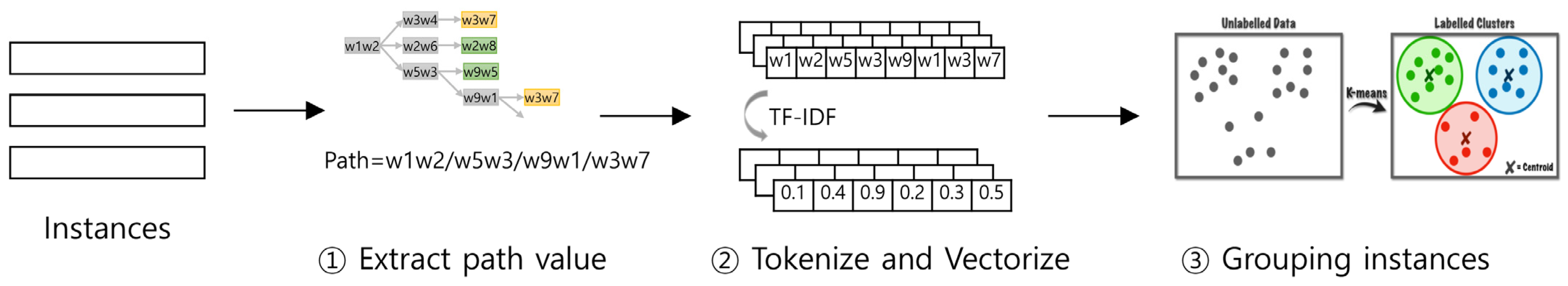
Large-scale software can exhibit different software characteristics among its subcomponents, each contributing to the overall functionality. In the software utilized in this study, which has over a thousand developers, the technical domains of the software are distinctly categorized into wireless protocols, NG protocols, operations management, and OS and middleware. By leveraging the file path information, the entire dataset is segmented into several groups with identical features. Cross-group performance measurements are then conducted to ascertain whether there are differences in characteristics among these groups. Figure 7 illustrates the method of instance grouping.
To separate groups using path information, the paths are tokenized into words and then vectorized using TF-IDF (term frequency-inverse document frequency) (②). Subsequently, K-NN clustering is applied to the vectorized path information to cluster similar paths into five groups (comprising four representative subsystem codes + miscellaneous code) (③). Defining groups in this manner allows for the identification of differences in characteristics among the groups. When such differences are observed, adding group information as a feature to the model can provide additional information, thereby potentially improving prediction performance. Table 7 shows the result of grouping the files.
4. Results
In this section, we undertake an examination of the four research questions (RQs) outlined in Section 3.1, utilizing knowledge derived from the results of our experiments.
Answer for RQ1.
How effectively does the software defect prediction (SDP) model anticipate defects?
Table 8 showcases the performance measurement outcomes of the XGB-based SDP model across six distinct scenarios. Initially, performance evaluation was conducted without any data preprocessing (①), followed by successive additions of scaling (②), outlier removal (③), class imbalance resolution through oversampling (④), the incorporation of new metrics (⑤), and, eventually, the addition of file type information (⑥). The ML-SDP exhibited optimal performance when comprehensive preprocessing was applied, incorporating all new features and employing the XGB classifier. In this scenario, the performance metrics were as follows: recall of 0.63, F-measurement of 0.74, and an ROC-AUC score of 0.87.
In comparison with prior studies, the predicted performance displayed notable variations, with some studies indicating higher performance and others demonstrating lower performance compared to our experiment. Table 9 provides a comparative analysis of our results with those from previous studies. Among 12 prior studies, including 7 on open-source projects and 5 on industrial domain projects, our study exhibited lower performance than 6 of the studies and comparable performance with 6 of the studies. Thus, it can be inferred that the ML-SDP model, developed using Samsung’s embedded software for telecommunication systems, has achieved a meaningful level of performance.
Answer for RQ2.
Did the incorporation of new features augment the performance of SDP?
Figure 8 provides a visual representation of the changes in predictive performance resulting from data processing and feature addition. Before incorporating the six new metrics and three source file types of information, the performance metrics were as follows: precision 0.51, recall 0.69, F-measurement 0.58, accuracy 0.78, and an ROC-AUC score of 0.84. Subsequently, after integrating the new metrics and source file type information, the performance metrics improved to: precision 0.55, recall 0.74, F-measurement 0.63, accuracy 0.80, and an ROC-AUC score of 0.87. After introducing the new metrics, all five indicators exhibited an improvement. Upon closer examination of the F-measure, there was a 6.90% increase from 0.58 to 0.62 (⑤) and, upon the inclusion of three additional source file types, four out of the five indicators showed further enhancement, resulting in a 1.72% increase from 0.62 to 0.63 (⑥). Overall, the total increase amounted to 0.86%. It is evident that the additional features introduced in this study significantly contributed to an enhancement of the predictive power of the SDP model.
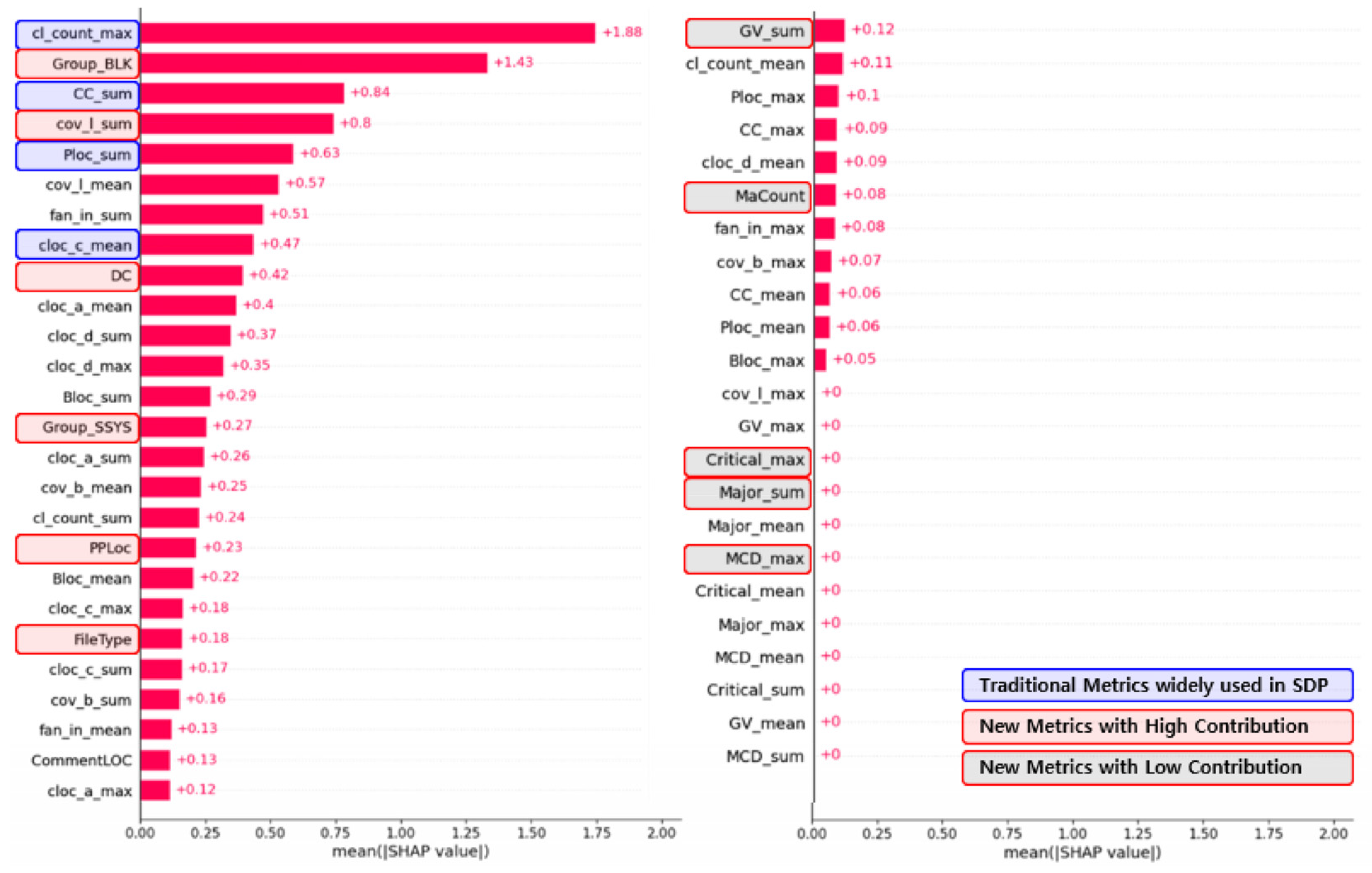
An examination of feature contributions, as depicted in Figure 9, reveals notable insights into the predictive power of various metrics. The contributions of traditional and widely used metrics in SDP, such as BLOC (build LOC), CLOC (changed LOC), and CC (cyclomatic complexity) remained high. However, some of the new features, such as Group_BLK, cov_l (line coverage), DC (duplicate code), Group_SSYS, and PPLOC also played an important role in improving prediction performance. Meanwhile, the GV, Critical/Major, and MCD features showed only minimal contributions.
Moreover, the Shapley value analysis underscored the pivotal role of certain quality metrics in capturing fault occurrence trends. Specifically, coverage, DC, and PPLOC displayed robust associations with fault occurrence, affirming their effectiveness as indicators for quality enhancement initiatives. Conversely, the GV, Critical/Major, and MCD features demonstrated minimal associations with fault occurrence, implying their limited utility in defect prediction scenarios. These findings provide actionable insights for prioritizing metrics and refining defect prediction strategies to bolster software quality.
Answer for RQ3.
How accurately does the SDP model forecast defects across different versions?
A comparative analysis of prediction performance across both same-version and cross-version scenarios yielded insightful observations. The precision metrics revealed that among the six cross-version predictions, four exhibited lower values than their same-version counterparts, while two displayed higher values. Similarly, the recall metrics indicated consistently lower performance across all six cross-version predictions. The F-measurement metrics exhibited lower values in five out of six cross-version cases and higher values in one case. Accuracy metrics followed a similar trend, with lower values observed in four cases and higher values in two cases compared to the same-version predictions (see Figure 10).
Overall, the average prediction performance under cross-version conditions demonstrated a notable decline across all five metrics compared to the same-version predictions. Particularly noteworthy was the average F-measurement (f1-score), which decreased from 0.62 for the same version to 0.54 for cross-version predictions, reflecting a significant 13% decrease in prediction performance (see Table 10).
The observed deterioration in prediction performance under cross-version conditions underscores the presence of distinct data characteristics among the different versions. It also suggests that the anticipated prediction performance under cross-version conditions is approximately 0.54, based on the F-measurement metric. These findings highlight the importance of considering version-specific nuances and adapting the prediction models accordingly to maintain optimal performance across diverse software versions.
Answer for RQ4.
Does predictive performance differ when segregating source files by type?
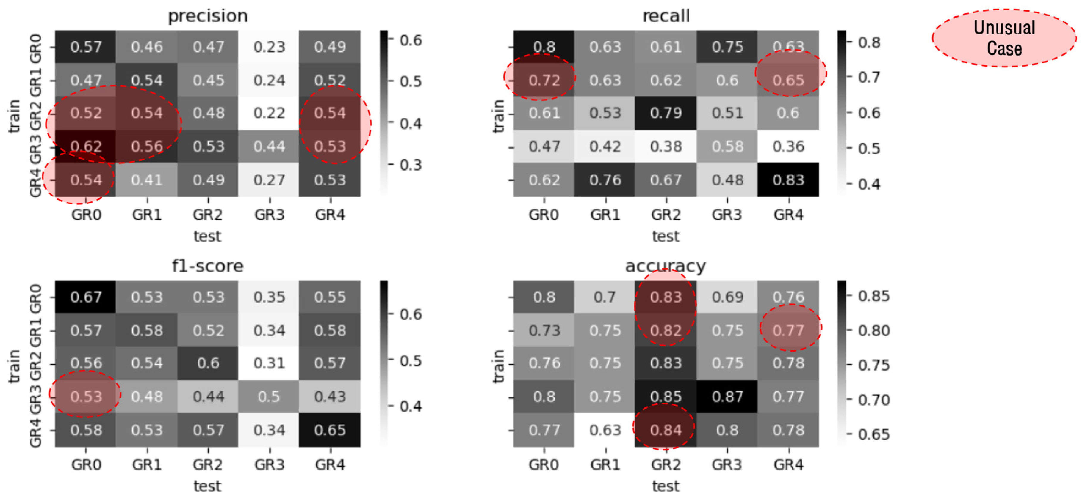
The analysis of prediction performance across cross-group scenarios revealed notable trends. Among the 20 cross-group predictions, 13 exhibited lower precision compared to the same group, while 7 showed higher precision. Similarly, 18 predictions demonstrated lower recall, with only 2 displaying higher values. The F-measurement scores followed a similar pattern, with 19 predictions showing lower values and 1 demonstrating improvement. Accuracy metrics indicated lower values in 16 cases and higher values in 4 cases compared to the same group predictions (see Figure 11).
On average, predictive performance under cross-group conditions was consistently lower across all five metrics compared to the same group predictions. Specifically, the average F-measurement for the same group was 0.60, while for cross-group predictions, it decreased to 0.50, reflecting a notable 17% decrease in predictive performance (see Table 11).
The observed decline in predictive performance under cross-group conditions underscores the significance of variations in data characteristics among different groups. To address this, we incorporated source file type information for group identification. Figure 8 demonstrates that the addition of source file type information resulted in a 1% improvement in precision, recall, and F-measurement metrics, indicating its effectiveness in enhancing prediction performance across diverse group scenarios.
5. Discussion and Conclusions
This study proposes an SDP model tailored for Samsung’s embedded software in telecommunication systems, yielding several significant results and implications. Firstly, it validates the applicability of SDP in the practical realm of embedded software in telecommunication systems. The model demonstrated moderate performance levels compared to the existing research, with an F-measurement of 0.63, a recall of 0.74, and an accuracy of 0.80. Secondly, specialized features like DC and PPLOC, which are specific to Samsung, were found to enhance predictive performance, leading to an increase in F-measurement from 0.58 to 0.62. Thirdly, the inclusion of information in three file types, namely, subsystem, block, and language identifiers, as features for machine learning training contributed to performance improvements, as evidenced by an increase in F-measurement from 0.62 to 0.63. Lastly, this study quantitatively confirmed the significance of Samsung’s software quality metrics as indicators of software quality, enhancing predictive performance when incorporated as features.
Our SDP model has been adopted in real-life projects to evaluate the effectiveness of software quality metrics, implement just-in-time buggy module detection [51], and enhance test efficiency through recommendations for buggy module-centric test cases. The model is intended to aid developers in identifying faulty modules early, understanding their causes, and making targeted improvements, such as removing duplicate code and optimizing preprocessing directives.
The study has successfully developed an ML-SDP model tailored to embedded software in telecommunication systems, highlighting its applicability in similar domains and the effectiveness of novel features. The findings of this study suggest that Samsung’s research outcomes are likely to be generalizable, as follows.
- This case study into embedded software for communication purposes provides empirical validation research results.
- Specialized features, such as PPLOC and DC, could serve as valuable indicators for software defect prediction and quality management in software that shares similar traits. These metrics hold a potential for application in analogous domains.
- If the proposed research methodology is concretized and tailored guidelines are established, this provides opportunities for the propagation of extension into domains with different characteristics.
However, several avenues for further research and expansion have been identified. Firstly, there is a crucial need to go into more depth regarding cases where the predicted values deviate from the actual values. Investigating such instances, pinpointing the underlying causes of discrepancies, and mitigating prediction errors can significantly enhance the accuracy of predictions. We plan to conduct in-depth investigations into cases where the predictions deviate, aiming to uncover new features influencing defect prediction. Secondly, it is imperative to explore the applicability of advanced methods that are known to enhance prediction performance in real-world industrial settings. One promising direction is the utilization of SDP models leveraging Transformer, a cutting-edge deep learning (DL) technology.
Author Contributions
Conceptualization, H.K. and S.D.; methodology, H.K. and S.D.; formal analysis, H.K.; investigation, H.K.; writing—original draft preparation, H.K.; writing—review and editing, S.D.; supervision, S.D. All authors have read and agreed to the published version of the manuscript.
Funding
This research received no external funding.
Institutional Review Board Statement
Not applicable.
Informed Consent Statement
Not applicable.
Data Availability Statement
Please contact the corresponding author or first author of this paper.
Acknowledgments
The authors wish to thank Dong-Kyu Lee, Senior Engineer, Software Engineering, Samsung Elec., for sharing software quality data for the thesis.
Conflicts of Interest
Author Hongkoo Kang was employed by the company SAMSUNG ELECTRONICS CO. Ltd. The remaining authors declare that the research was conducted in the absence of any commercial or financial relationships that could be construed as a potential conflict of interest.
References
- Antinyan, V. Revealing the Complexity of Automotive Software. In Proceedings of the 28th ACM Joint Meeting on European Software Engineering Conference and Symposium on the Foundations of Software Engineering, Virtual Event USA, 8 November 2020; pp. 1525–1528. [Google Scholar]
- Stradowski, S.; Madeyski, L. Exploring the Challenges in Software Testing of the 5G System at Nokia: A Survey. Inf. Softw. Technol. 2023, 153, 107067. [Google Scholar] [CrossRef]
- Wahono, R.S. A Systematic Literature Review of Software Defect Prediction: Research Trends, Datasets, Methods and Frameworks. J. Softw. Eng. 2015, 1, 1–16. [Google Scholar]
- IEEE Std 610.12-1990; IEEE Standard Glossary of Software Engineering Terminology. IEEE: Manhattan, NY, USA, 1990; pp. 1–84. [CrossRef]
- Shafiq, M.; Alghamedy, F.H.; Jamal, N.; Kamal, T.; Daradkeh, Y.I.; Shabaz, M. Scientific Programming Using Optimized Machine Learning Techniques for Software Fault Prediction to Improve Software Quality. IET Softw. 2023, 17, 694–704. [Google Scholar] [CrossRef]
- Iqbal, A.; Aftab, S.; Ali, U.; Nawaz, Z.; Sana, L.; Ahmad, M.; Husen, A. Performance Analysis of Machine Learning Techniques on Software Defect Prediction Using NASA Datasets. Int. J. Adv. Sci. Comput. Appl. 2019, 10, 300–308. [Google Scholar] [CrossRef]
- Paramshetti, P.; Phalke, D.A. Survey on Software Defect Prediction Using Machine Learning Techniques. Int. J. Sci. Res. 2012, 3, 1394–1397. [Google Scholar]
- Thota, M.K.; Shajin, F.H.; Rajesh, P. Survey on Software Defect Prediction Techniques. Int. J. Appl. Sci. Eng. 2020, 17, 331–344. [Google Scholar] [CrossRef] [PubMed]
- Durelli, V.H.S.; Durelli, R.S.; Borges, S.S.; Endo, A.T.; Eler, M.M.; Dias, D.R.C.; Guimarães, M.P. Machine Learning Applied to Software Testing: A Systematic Mapping Study. IEEE Trans. Reliab. 2019, 68, 1189–1212. [Google Scholar] [CrossRef]
- Stradowski, S.; Madeyski, L. Machine Learning in Software Defect Prediction: A Business-Driven Systematic Mapping Study. Inf. Softw. Technol. 2023, 155, 107128. [Google Scholar] [CrossRef]
- Stradowski, S.; Madeyski, L. Industrial Applications of Software Defect Prediction Using Machine Learning: A Business-Driven Systematic Literature Review. Inf. Softw. Technol. 2023, 159, 107192. [Google Scholar] [CrossRef]
- Kamei, Y.; Shihab, E.; Adams, B.; Hassan, A.E.; Mockus, A.; Sinha, A.; Ubayashi, N. A Large-Scale Empirical Study of Just-in-Time Quality Assurance. IEEE Trans. Softw. Eng. 2013, 39, 757–773. [Google Scholar] [CrossRef]
- Menzies, T.; Greenwald, J.; Frank, A. Data Mining Static Code Attributes to Learn Defect Predictors. IEEE Trans. Softw. Eng. 2007, 33, 2–13. [Google Scholar] [CrossRef]
- Catal, C.; Diri, B. A Systematic Review of Software Fault Prediction Studies. Expert Syst. Appl. 2009, 36, 7346–7354. [Google Scholar] [CrossRef]
- Amasaki, S.; Takagi, Y.; Mizuno, O.; Kikuno, T. A Bayesian Belief Network for Assessing the Likelihood of Fault Content. In Proceedings of the 14th International Symposium on Software Reliability Engineering, Denver, CO, USA, 17–20 November 2003; pp. 215–226. [Google Scholar]
- Akmel, F.; Birihanu, E.; Siraj, B. A Literature Review Study of Software Defect Prediction Using Machine Learning Techniques. Int. J. Emerg. Res. Manag. Technol. 2018, 6, 300. [Google Scholar] [CrossRef]
- Khan, M.J.; Shamail, S.; Awais, M.M.; Hussain, T. Comparative Study of Various Artificial Intelligence Techniques to Predict Software Quality. In Proceedings of the 2006 IEEE International Multitopic Conference, Islamabad, Pakistan, 23–24 December 2006; pp. 173–177. [Google Scholar]
- Kim, S.; Zimmermann, T.; Whitehead, E.J., Jr.; Zeller, A. Predicting Faults from Cached History. In Proceedings of the 29th International Conference on Software Engineering (ICSE’07), Minneapolis, MN, USA, 20–26 May 2007; pp. 489–498. [Google Scholar]
- Hassan, A.E. Predicting Faults Using the Complexity of Code Changes. In Proceedings of the 2009 IEEE 31st International Conference on Software Engineering, Vancouver, BC, Canada, 16 May 2009; pp. 78–88. [Google Scholar]
- Khoshgoftaar, T.M.; Seliya, N. Tree-Based Software Quality Estimation Models for Fault Prediction. In Proceedings of the Eighth IEEE Symposium on Software Metrics, Ottawa, ON, Canada, 4–7 June 2002; pp. 203–214. [Google Scholar]
- Li, J.; He, P.; Zhu, J.; Lyu, M.R. Software Defect Prediction via Convolutional Neural Network. In Proceedings of the 2017 IEEE International Conference on Software Quality, Reliability and Security (QRS), Prague, Czech Republic, 25–29 July 2017; IEEE: Prague, Czech Republic, 2017; pp. 318–328. [Google Scholar]
- Chen, J.; Hu, K.; Yu, Y.; Chen, Z.; Xuan, Q.; Liu, Y.; Filkov, V. Software Visualization and Deep Transfer Learning for Effective Software Defect Prediction. In Proceedings of the ACM/IEEE 42nd International Conference on Software Engineering, Seoul, Republic of Korea, 27 June 2020; pp. 578–589. [Google Scholar]
- Malhotra, R.; Jain, A. Fault Prediction Using Statistical and Machine Learning Methods for Improving Software Quality. J. Inf. Process. Syst. 2012, 8, 241–262. [Google Scholar] [CrossRef]
- Chidamber, S.R.; Kemerer, C.F. A Metrics Suite for Object Oriented Design. IEEE Trans. Softw. Eng. 1994, 20, 476–493. [Google Scholar] [CrossRef]
- Lee, S.; Kim, T.-K.; Ryu, D.; Baik, J. Software Defect Prediction with new Image Conversion Technique of Source Code. J. Korean Inst. Inf. Sci. Eng. 2021, 239–241. Available online: https://www.dbpia.co.kr/journal/articleDetail?nodeId=NODE11112825 (accessed on 21 October 2023).
- Sojeong, K.; Eunjung, J.; Jiwon, C.; Ryu, D. Software Defect Prediction Based on Ft-Transformer. J. Korean Inst. Inf. Sci. Eng. 2022, 1770–1772. Available online: https://www-dbpia-co-kr.translate.goog/journal/articleDetail?nodeId=NODE11113815&_x_tr_sl=ko&_x_tr_tl=en&_x_tr_hl=en&_x_tr_pto=sc (accessed on 21 October 2023).
- Choi, J.; Lee, J.; Ryu, D.; Kim, S. Identification of Generative Adversarial Network Models Suitable for Software Defect Prediction. J. KIISE 2022, 49, 52–59. [Google Scholar] [CrossRef]
- Lee, J.; Choi, J.; Ryu, D.; Kim, S. TabNet based Software Defect Prediction. J. Korean Inst. Inf. Sci. Eng. 2021, 1255–1257. Available online: https://www.dbpia.co.kr/journal/articleDetail?nodeId=NODE11036011&nodeId=NODE11036011&medaTypeCode=185005&isPDFSizeAllowed=true&locale=ko&foreignIpYn=Y&articleTitle=TabNet+%EA%B8%B0%EB%B0%98%EC%9D%98+%EC%86%8C%ED%94%84%ED%8A%B8%EC%9B%A8%EC%96%B4+%EA%B2%B0%ED%95%A8+%EC%98%88%EC%B8%A1&articleTitleEn=TabNet+based+Software+Defect+Prediction&language=ko_KR&hasTopBanner=true (accessed on 21 October 2023).
- Zhang, Q.; Wu, B. Software Defect Prediction via Transformer. In Proceedings of the 2020 IEEE 4th Information Technology, Networking, Electronic and Automation Control Conference (IT-NEC), Chongqing, China, 12–14 June 2020; pp. 874–879. [Google Scholar]
- Qureshi, M.R.J.; Qureshi, W.A. Evaluation of the Design Metric to Reduce the Number of Defects in Software Development. Int. J. Inf. Technol. Converg. Serv. 2012, 4, 9–17. [Google Scholar] [CrossRef]
- Xing, F.; Guo, P.; Lyu, M.R. A Novel Method for Early Software Quality Prediction Based on Support Vector Machine. In Proceedings of the 16th IEEE International Symposium on Software Reliability Engineering (ISSRE’05), Chicago, IL, USA, 8–11 November 2005; pp. 10–222. [Google Scholar]
- Tosun, A.; Turhan, B.; Bener, A. Practical Considerations in Deploying AI for Defect Prediction: A Case Study within the Turkish Telecommunication Industry. In Proceedings of the 5th International Conference on Predictor Models in Software Engineering, Vancouver, BC, Canada, 18 May 2009; Association for Computing Machinery: New York, NY, USA, 2009; pp. 1–9. [Google Scholar]
- Kim, M.; Nam, J.; Yeon, J.; Choi, S.; Kim, S. REMI: Defect Prediction for Efficient API Testing. In Proceedings of the 2015 10th Joint Meeting on Foundations of Software Engineering, Bergamo, Italy, 30 August 2015; pp. 990–993. [Google Scholar]
- Kim, D.; Lee, S.; Seong, G.; Kim, D.; Lee, J.; Bhae, H. An Experimental Study on Software Fault Prediction considering Engineering Metrics based on Machine Learning in Vehicle. In Proceedings of the Korea Society of Automotive Engineers Fall Conference and Exhibition, Jeju, Republic of Korea, 18–21 November 2020; pp. 552–559. [Google Scholar]
- Kang, J.; Ryu, D.; Baik, J. A Case Study of Industrial Software Defect Prediction in Maritime and Ocean Transportation Industries. J. KIISE 2020, 47, 769–778. [Google Scholar] [CrossRef]
- McCabe, T.J. A Complexity Measure. IEEE Trans. Softw. Eng. 1976, SE-2, 308–320. [Google Scholar] [CrossRef]
- Huang, F.; Liu, B. Software Defect Prevention Based on Human Error Theories. Chin. J. Aeronaut. 2017, 30, 1054–1070. [Google Scholar] [CrossRef]
- ETSI TS 138 401. Available online: https://www.etsi.org/deliver/etsi_ts/138400_138499/138401/17.01.01_60/ts_138401v170101p.pdf (accessed on 21 October 2023).
- Han, I. Communications of the Korean Institute of Information Scientists and Engineers. Young 2013, 31, 56–62. [Google Scholar]
- Shin, H.J.; Song, J.H. A Study on Embedded Software Development Method (TBESDM: Two-Block Embedded Software Development Method). Soc. Converg. Knowl. Trans. 2020, 8, 41–49. [Google Scholar]
- Friedman, M.A.; Tran, P.Y.; Goddard, P.L. Reliability Techniques for Combined Hardware and Software Systems; Defense Technical Information Center: Fort Belvoir, VA, USA, 1992. [Google Scholar]
- Lee, S.; No, H.; Lee, S.; Lee, W.J. Development of Code Suitability Analysis Tool for Embedded Software Module. J. Korean Inst. Inf. Sci. Eng. 2015, 1582–1584. Available online: https://www.dbpia.co.kr/journal/articleDetail?nodeId=NODE06602802 (accessed on 21 October 2023).
- Lee, E. Definition of Check Point for Reliability Improvement of the Embedded Software. J. Secur. Eng. Res. 2011, 8, 149–156. [Google Scholar]
- Moser, R.; Pedrycz, W.; Succi, G. A Comparative Analysis of the Efficiency of Change Metrics and Static Code Attributes for Defect Prediction. In Proceedings of the 13th International Conference on Software Engineering—ICSE ’08; ACM Press: Leipzig, Germany, 2008; p. 181. [Google Scholar]
- Chawla, N.V.; Bowyer, K.W.; Hall, L.O.; Kegelmeyer, W.P. SMOTE: Synthetic Minority Over-Sampling Technique. J. Artif. Intell. Res. 2002, 16, 321–357. [Google Scholar] [CrossRef]
- SMOTE—Version 0.11.0. Available online: https://imbalanced-learn.org/stable/references/generated/imblearn.over_sampling.SMOTE.html (accessed on 15 October 2023).
- Yoo, B.J. A Study on the Performance Comparison and Approach Strategy by Classification Methods of Imbalanced Data. Korean Data Anal. Soc. 2021, 23, 195–207. [Google Scholar] [CrossRef]
- Introduction to Boosted Trees—Xgboost 2.0.0 Documentation. Available online: https://xgboost.readthedocs.io/en/stable/tutorials/model.html (accessed on 21 October 2023).
- Molnar, C. 9.5 Shapley Values|Interpretable Machine Learning. Available online: https://christophm.github.io/interpretable-ml-book/shapley.html (accessed on 21 October 2023).
- Lundberg, S.M.; Lee, S.-I. A Unified Approach to Interpreting Model Predictions. In Proceedings of the Advances in Neural Information Processing Systems; Curran Associates Inc.: Glasgow, Scotland, 2017; Volume 30. [Google Scholar]
- Zhao, Y.; Damevski, K.; Chen, H. A Systematic Survey of Just-in-Time Software Defect Prediction. ACM Comput. Surv. 2023, 55, 1–35. [Google Scholar] [CrossRef]
Figure 1.
Machine learning-based software defect prediction.

Figure 2.
Software components of the base station.

Figure 3.
Continuous new version software development for the base station.

Figure 4.
The experiments for developing the SDP model.

Figure 5.
Data collection and defect prediction across versions.

Figure 6.
Updating quality metrics based on defects identified in the system test.

Figure 7.
Grouping instances using TF-IDF and K-means (revised).

Figure 8.
The changes in predictive performance due to data preprocessing and feature addition.

Figure 9.
Shapley values of the XGB model.

Figure 10.
Prediction performance under cross-version conditions.

Figure 11.
Prediction performance under cross-group conditions.


Table 1.
Overview of studies applied in open-source projects.
| Studies | Data | Buggy Rate (%) | Granularity | Feature | Model | Evaluation |
|---|---|---|---|---|---|---|
| [5] | PC1 | Unknown | Unknown | Complexity, LOC | ACO-SVM | Precision 0.99, Recall 0.98, F-Measure 0.99 |
| [23] | Apache POI | 63.57 | Class | OO-Metric [24], Complexity, LOC | Bagging, … | Recall 0.83, Precision 0.82, AUC 0.876 |
| [25] | jEdit Lucene log4j Xalan Poi | 19.2~49.7 | File | Image of Source Code | DTL-DP | F-Measure 0.58~0.82, Accuracy 0.70~0.86 |
| [26] | AEEEM Relink | 9.26~50.52 | Class | Complexity, LOC | Ft-Transformer | Recall 0.77 |
| [27] | AEEEM AUDI JIRA | 4~40 | Unknown | Complexity LOC | Unknown | F-Measure 0.50~0.86 |
| [28] | AEEEM AUDI | 2.11~39.81 | Class, File | - | TabNet | Recall 0.85 |
| [29] | Camel Lucene Synapse Xerces Jedit Xalan Poi | 15.7~64.2 | File | AST (Abstract Syntax Tree) | Transformer | F-Measure Average 0.626 |
Table 2.
Overview of studies applied in real industrial domains.
| Studies | Data | Buggy Rate (%) | Granularity | Feature | Model | Evaluation |
|---|---|---|---|---|---|---|
| [31] | MIS | Unknown | Unknown | Complexity LOC | TSVM | Accuracy 0.90 |
| [32] | GSM+ NASA | Avg 0.3~1 | File | Complexity LOC | Naïve Bayes | Recall Average 0.90 |
| [33] | Tizen API | Unknown | API | OO-Metric Complexity LOC | Random Forest | Precision 0.8 Recall 0.7 F-measure 0.75 |
| [34] | Software in Vehicle | 17.6 | Class | Complexity LOC Engineering-Metric | Random Forest | Accuracy 0.96 F-measure 0.90 AUC 0.92 |
| [35] | Software in the maritime and ocean transportation industries | Unknown | Unknown | Diffusion LOC Purpose History Experience | Random Forest | Accuracy 0.91 Precision 0.86 Recall 0.80 F-Measure 0.83 |
Table 3.
The distribution of base station software development data across versions.
| Version | Samples (Files) | Buggy Files | Buggy Rate | Sample Rate | Code Submitter | Feature Count | Dev. Period |
|---|---|---|---|---|---|---|---|
| V1 | 4282 | 1126 | 26.3% | 42% | 897 | 353 | 3M |
| V2 | 4637 | 1575 | 34.0% | 40% | 1159 | 642 | 6M |
| V3 | 8808 | 1292 | 14.7% | 74% | 1098 | 568 | 6M |
| Sum | 17,727 | 3993 | - | - | - | - | - |
| Average | 5909 | 1331 | 22.5% | - | - | - | - |
Table 4.
The distribution of base station software development data across programming languages.
| Language | Samples (Files) | Buggy Files | Buggy Rate |
|---|---|---|---|
| C | 8585 | 2188 | 20.3% |
| C++ | 5149 | 1805 | 26.0% |
| Sum | 17,727 | 3993 | - |
| Average | 5909 | 1331 | 22.5% |
Table 5.
Product metrics and process metrics.
| No | Metric Type | Feature Name | Definition | Comments |
|---|---|---|---|---|
| 1 | Product Metric | Ploc | Physical LOC | min/max/sum |
| 2 | Bloc | Build LOC | min/max/sum | |
| 3 | CommentLOC | Comment LOC | ||
| 4 | fan_in | Fan In | min/max/sum | |
| 5 | CC | Cyclomatic Complexity | min/max/sum | |
| 6 | GV 1 | Global Variables accessing to | min/max/sum | |
| 7 | MCD 1 | Module Circular Dependency | min/max/sum | |
| 8 | DC 1 | Duplicate Code | ||
| 9 | PPLOC 1 | Preprocessor LOC | ||
| 10 | Process Metric | cl_count | Change List Count | min/max/sum |
| 11 | cloc_a | Added LOC | min/max/sum | |
| 12 | cloc_c | Changed LOC | min/max/sum | |
| 13 | cloc_d | Deleted LOC | min/max/sum | |
| 14 | cov_l, cov_b 1 | Line/Branch Coverage | min/max/sum | |
| 15 | Critical/Major 1 | Static Analysis Defect | ||
| 16 | FileType1 1 | Programming Language Type | ||
| 17 | Group_SSYS 1 | Subsystem ID | 0~4 | |
| 18 | Group_BLK 1 | Block ID | 0~99 |
1 indicates metrics that have been newly introduced in the current research.
Table 6.
Confusion matrix.
| Confusion Matrix | Predicted Class | ||
|---|---|---|---|
| Buggy (Positive) | Clean (Negative) | ||
| Actual Class | Buggy | TP (True Positive) | FN (False Negative) |
| Clean | FP (False Positive) | TN (True Negative) | |
Table 7.
Distribution of the base station software data groups (subsystems).
| Group | Samples (Files) | Buggy Files | Buggy Rate |
|---|---|---|---|
| G0 | 3999 | 1321 | 24.8% |
| G1 | 3477 | 1319 | 27.5% |
| G2 | 1743 | 328 | 15.8% |
| G3 | 2118 | 263 | 11.0% |
| G4 | 2397 | 762 | 24.1% |
| Sum | 17,727 | 3993 | 22.5% |
Table 8.
Performance assessment result for the SDP model.
| Classifier | ① No Processing | ② Scaling | ||||||||
| Precision | Recall | F-measurement | Accuracy | ROC-AUC | Precision | Recall | F-measurement | Accuracy | ROC-AUC | |
| RF | 0.69 | 0.41 | 0.52 | 0.83 | 0.85 | 0.69 | 0.41 | 0.52 | 0.83 | 0.85 |
| LR | 0.63 | 0.39 | 0.49 | 0.81 | 0.76 | 0.71 | 0.34 | 0.46 | 0.82 | 0.83 |
| XGB | 0.63 | 0.45 | 0.53 | 0.82 | 0.85 | 0.63 | 0.45 | 0.53 | 0.82 | 0.85 |
| MLP | 0.44 | 0.25 | 0.32 | 0.76 | 0.54 | 0.49 | 0.47 | 0.48 | 0.77 | 0.75 |
| Classifier | ③ Outlier Processing | ④ Oversampling | ||||||||
| Precision | Recall | F-measurement | Accuracy | ROC-AUC | Precision | Recall | F-measurement | Accuracy | ROC-AUC | |
| RF | 0.67 | 0.4 | 0.5 | 0.82 | 0.85 | 0.49 | 0.74 | 0.59 | 0.77 | 0.85 |
| LR | 0.58 | 0.42 | 0.49 | 0.80 | 0.8 | 0.42 | 0.78 | 0.55 | 0.71 | 0.81 |
| XGB | 0.64 | 0.47 | 0.54 | 0.82 | 0.85 | 0.51 | 0.69 | 0.58 | 0.78 | 0.84 |
| MLP | 0.42 | 0.41 | 0.41 | 0.74 | 0.65 | 0.39 | 0.41 | 0.4 | 0.72 | 0.61 |
| Classifier | ⑤ Additional Metric | ⑥ Sample Grouping | ||||||||
| Precision | Recall | F-measurement | Accuracy | ROC-AUC | Precision | Recall | F-measurement | Accuracy | ROC-AUC | |
| RF | 0.5 | 0.76 | 0.6 | 0.78 | 0.86 | 0.52 | 0.75 | 0.61 | 0.79 | 0.86 |
| LR | 0.42 | 0.62 | 0.5 | 0.72 | 0.72 | 0.42 | 0.62 | 0.5 | 0.72 | 0.72 |
| XGB | 0.54 | 0.73 | 0.62 | 0.8 | 0.86 | 0.55 | 0.74 | 0.63 | 0.80 | 0.87 |
| MLP | 0.39 | 0.3 | 0.34 | 0.74 | 0.51 | 0.45 | 0.25 | 0.32 | 0.76 | 0.5 |
Table 9.
Performance comparison with prior studies.
| Studies | Precision | Recall | F-Measurement | Accuracy | ROC-AUC | Data |
|---|---|---|---|---|---|---|
| [5] | 0.99 | 0.98 | 0.99 | - | - | PC1 |
| [23] | 0.82 | 0.83 | - | - | 0.88 | Apache |
| [25] | - | - | 0.58~0.82 | 0.70~0.86 | - | iEdit, … |
| [26] | - | 0.77 | - | - | - | AEEEM, … |
| [27] | - | - | 0.50~0.86 | - | - | AEEEM, … |
| [28] | - | 0.50 | - | - | - | AEEEM, … |
| [29] | - | - | 0.626 | - | - | Camel, … |
| [31] | - | - | - | 0.90 | - | MIS |
| [32] | - | 0.90 | - | - | - | GSM, NASA |
| [33] | 0.80 | 0.70 | 0.75 | - | - | Tizen API |
| [34] | - | - | 0.90 | 0.96 | 0.92 | Vehicle S/W |
| [35] | 0.86 | 0.80 | 0.83 | 0.91 | - | Ship S/W |
| This study | 0.55 | 0.74 | 0.63 | 0.80 | 0.87 | Samsung |
Table 10.
Comparison of prediction performance under cross-version conditions.
| Case | Precision | Recall | F-Measurement | Accuracy | ROC-AUC |
|---|---|---|---|---|---|
| Average for Within-Version | 0.55 | 0.72 | 0.62 | 0.79 | 0.86 |
| Average for Cross-Version | 0.52 | 0.62 | 0.54 | 0.76 | 0.81 |
Table 11.
Comparison of prediction performance under cross-group conditions.
| Case | Precision | Recall | F-Measurement | Accuracy | ROC-AUC |
|---|---|---|---|---|---|
| Average of Within-Group | 0.51 | 0.73 | 0.60 | 0.81 | 0.85 |
| Average of Cross-Group | 0.46 | 0.58 | 0.50 | 0.77 | 0.79 |
Disclaimer/Publisher’s Note: The statements, opinions and data contained in all publications are solely those of the individual author(s) and contributor(s) and not of MDPI and/or the editor(s). MDPI and/or the editor(s) disclaim responsibility for any injury to people or property resulting from any ideas, methods, instructions or products referred to in the content. |
© 2024 by the authors. Licensee MDPI, Basel, Switzerland. This article is an open access article distributed under the terms and conditions of the Creative Commons Attribution (CC BY) license (https://creativecommons.org/licenses/by/4.0/).
Share and Cite
MDPI and ACS Style
Kang, H.; Do, S. ML-Based Software Defect Prediction in Embedded Software for Telecommunication Systems (Focusing on the Case of SAMSUNG ELECTRONICS). Electronics 2024, 13, 1690. https://doi.org/10.3390/electronics13091690
AMA Style
Kang H, Do S. ML-Based Software Defect Prediction in Embedded Software for Telecommunication Systems (Focusing on the Case of SAMSUNG ELECTRONICS). Electronics. 2024; 13(9):1690. https://doi.org/10.3390/electronics13091690
Chicago/Turabian StyleKang, Hongkoo, and Sungryong Do. 2024. "ML-Based Software Defect Prediction in Embedded Software for Telecommunication Systems (Focusing on the Case of SAMSUNG ELECTRONICS)" Electronics 13, no. 9: 1690. https://doi.org/10.3390/electronics13091690
Note that from the first issue of 2016, this journal uses article numbers instead of page numbers. See further details here.