Feasibility of a Stochastic Collaborative Beamforming for Long Range Communications in Wireless Sensor Networks

 ,
,  , , and
Abstract
:1. Introduction
2. Related Work
2.1. Beamforming
2.2. Practical Implementations
2.3. Energy Issues
3. Maximum Distance between Motes in Experimental Deployments
4. Cooperative Stochastic Transmission Planning
| Algorithm: Iterative Algorithm of Stochastic Cooperative Transmission |
| (WSN is synchronized after receiving the signal from the BS) |
| WSN monitoring |
| WSN motes ← The BS sends a signal requesting transmission of monitored data |
| The motes that receive the BS signal choose a coordinator |
| The motes are synchronized ← clocks |
| The motes share the monitored data |
| while(BS does not receive the message)do |
| BS ← Motes send message with data |
| BS sends signal with acknowledgement of receipt ← if BS receives the message |
| end |
| WSN motes stop transmission |
| WSN monitoring continues |
4.1. Array Theory Concepts
4.2. SCB from a WSN with Linear Distribution of Motes in Horizontal Plane
4.2.1. Uniform Linear Distribution
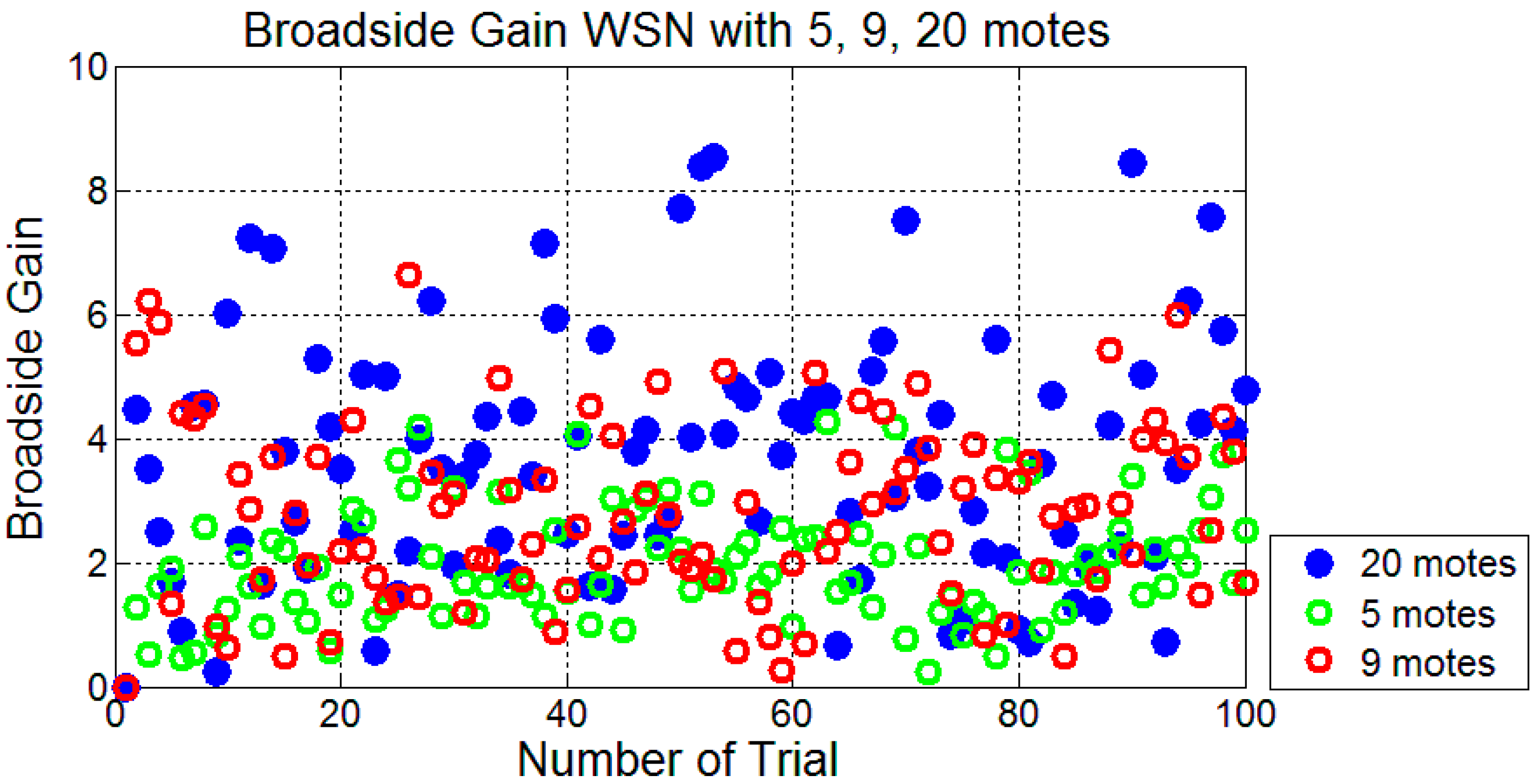
4.2.2. Random Linear Distribution and Stochastic Transmission Activation
4.3. WSN with Two-Dimensional Distribution
5. Conclusions
Author Contributions
Funding
Conflicts of Interest
References
- IEEE. TaskGroup 4 Standard 802.15.4-2006. Available online: http://www.ieee802.org/15/pub/TG4.html (accessed on 17 October 2018).
- Strazdins, G.; Elsts, A.; Nesenbergs, K.; Selavo, L. Wireless Sensor Network Operating System Design Rules Based on Real-World Deployment Survey. J. Sens. Actuator Netw. 2013, 2, 509–556. [Google Scholar] [CrossRef] [Green Version]
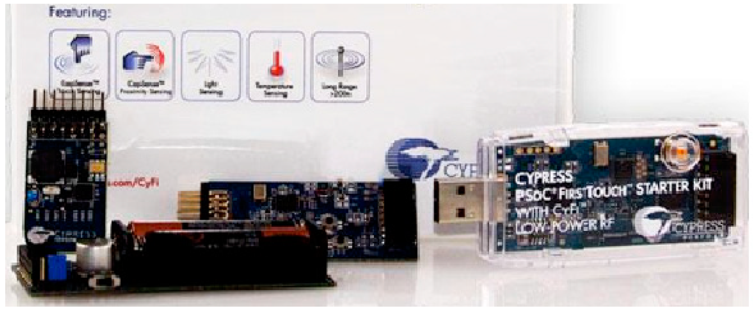
- Cypress CY3271 Kit. Available online: http://www.cypress.com/products/cyfi-low-power-rf (accessed on 17 October 2018).
- Brown, D.R.; Poor, H.V. Time-slotted round-trip carrier synchronization ford is tribute beamforming. IEEE Trans. Signal Process. 2008, 56, 5630–5643. [Google Scholar] [CrossRef]
- Ochiai, H.; Mitran, P.; Poor, H.V.; Tarokh, V. Collaborative beamforming for distributed wireless ad hoc sensor networks. IEEE Trans. Signal Process. 2005, 53, 4110–4124. [Google Scholar] [CrossRef] [Green Version]
- Mudumbai, R.; Brown, D.R.; Madhow, U.; Poor, H.V. Distributed Transmit Beamforming: Challenges and Recent Progress. Commun. Mag. 2009, 47, 102–110. [Google Scholar] [CrossRef]
- Ochiai, H.; Imai, H. Collaborative Beamforming. In New Directions in Wireless Communications Research; Springer: Boston, MA, USA, 2009; pp. 175–197. [Google Scholar]
- Song, S.; Thompson, J.S.; Chung, P.J.; Grant, P.M. BER Analysis for Distributed Beamforming with Phase Errors. IEEE Trans. Veh. Technol. 2010, 59, 4169–4174. [Google Scholar] [CrossRef]
- Mudumbai, R.; Barriac, G.; Madhow, U. On the feasibility of distributed beamforming in wireless networks. IEEE Trans. Wirel. Commun. 2007, 6, 1754–1763. [Google Scholar] [CrossRef]
- Noh, K.L.; Chaudhari, Q.M.; Serpedin, E.; Suter, B.W. Novel Clock Phase Offset and Skew Estimation Using Two-Way Timing Message Exchanges for Wireless Sensor Networks. IEEE Trans. Commun. 2007, 55, 766–777. [Google Scholar] [CrossRef]
- Kim, J.S.; Lee, J.; Serpedin, E.; Qaraqe, K. Robust Clock Synchronization in Wireless Sensor Networks through Noise Density Estimation. IEEE Trans. Signal Process. 2011, 59, 3035–3047. [Google Scholar] [CrossRef]
- Huang, G.; Zomaya, A.Y.; Delicato, F.C.; Pires, P.F. An accurate on-demand time synchronization protocol for wireless sensor networks. J. Parallel Distrib. Comput. 2012, 72, 1332–1346. [Google Scholar] [CrossRef]
- Schmid, T.; Shea, R.; Charbiwala, Z.; Friedman, J.; Srivastava, M.B.; Cho, Y.H. On the interaction of clocks, power, and synchronization in duty-cycled embedded sensor nodes. ACM Trans. Sens. Netw. 2010, 7, 24. [Google Scholar] [CrossRef]
- Felici-Castell, S.; Navarro, E.A.; Pérez-Solano, J.J.; Segura-García, J.; García-Pineda, M. Practical Considerations in the Implementation of Collaborative Beamforming on Wireless Sensor Networks. Sensors 2017, 17, 237. [Google Scholar] [CrossRef]
- Ochiai, H.; Mitran, P.; Poor, H.V.; Tarokh, V. Collaborative beam forming in ad hoc networks. In Proceedings of the IEEE Information Theory Workshop, San Antonio, TX, USA, 24–29 October 2004; pp. 396–401. [Google Scholar]
- Barriac, G.; Mudumbai, R.; Madhow, U. Distributed beamforming for information transfer in sensor networks. In Proceedings of the 3rd International Symposium on Information Processing in Sensor Networks, Berkeley, CA, USA, 26–27 April 2004; pp. 81–88. [Google Scholar]
- Tsinos, C.G.; Vlachos, E.; Berberidis, K. Distributed blind adaptive computation of beamforming weights for relay networks. In Proceedings of the 2013 IEEE 24th Annual International Symposium on Personal, Indoor, and Mobile Radio Communications (PIMRC), London, UK, 8–11 September 2013; pp. 570–574. [Google Scholar]
- Tsinos, C.G.; Ottersten, B. An Efficient Algorithm for Unit-Modulus Quadratic Programs with Application in Beamforming for Wireless Sensor Networks. IEEE Signal Process. Lett. 2018, 25, 169–173. [Google Scholar] [CrossRef]
- Mudumbai, R.; Hespanha, J.; Madhow, U.; Barriac, G. Scalable feedback control for distributed beamforming in sensor networks. In Proceedings of the International Symposium on Information Theory, Adelaide, SA, Australia, 4–9 September 2005; pp. 137–141. [Google Scholar]
- Mudumbai, R.; Wild, B.; Madhow, U.; Ramchandran, K. Distributed beamforming using 1 bit feedback: From concept to realization. In Proceedings of the IEEE 44th Allerton Conference on Communication, Control and Computing, Monticello, IL, USA, 27–29 September 2006; pp. 1020–1027. [Google Scholar]
- Shi, S.; Zhu, S.; Gu, X.; Hu, R. Extendable carrier synchronization for distributed beamforming in wireless sensor networks. In Proceedings of the 2016 International Wireless Communications and Mobile Computing Conference (IWCMC), Paphos, Cyprus, 5–9 September 2016; pp. 298–303. [Google Scholar]
- Uher, J.; Wysoki, T.A.; Wysoki, B.J. Review of distributed beamforming. J. Telecommun. Inf. Technol. 2011, 1, 78–88. [Google Scholar]
- Ahmed, M.F.A.; Vorobyov, S.A. Performance characteristics of collaborative beamforming for wireless sensor networks with Gaussian distributed sensor nodes. In Proceedings of the 2008 IEEE International Conference on Acoustics, Speech and Signal Processing, Las Vegas, NV, USA, 31 March–4 April 2008; pp. 3249–3252. [Google Scholar]
- Ahmed, M.F.A.; Vorobyov, S.A. Collaborative beamforming for wireless sensor networks with Gaussian distributed sensor nodes. IEEE Trans. Wirel. Commun. 2009, 8, 638–643. [Google Scholar] [CrossRef]
- Zarifi, K.; Affes, S.; Ghrayeb, A. Distributed beamforming for wireless sensor networks with random node location. In Proceedings of the 2009 IEEE International Conference on Acoustics, Speech and Signal Processing, Taipei, Taiwan, 19–24 April 2009; pp. 2261–2264. [Google Scholar]
- Huang, J.; Wang, P.; Wan, Q. Collaborative beamforming for wireless sensor networks with arbitrary distributed sensors. IEEE Commun. Lett. 2012, 16, 1118–1120. [Google Scholar] [CrossRef]
- Matamoros, J.; Anton-Haro, C.; Gregoratti, D.; Berbakov, L. Distributed beampattern control with one-bit of feedback. In Proceedings of the 20th European Wireless Conference European Wireless 2014, Barcelona, Spain, 14–16 May 2014; pp. 1–5. [Google Scholar]
- NikAbdMalik, N.; Esa, M.; Latiff, N.M.A. Least-square collaborative beamforming linear array for steering capability in green wireless sensor networks. J. Electron. Sci. Technol. 2016, 14, 118–124. [Google Scholar]
- Sun, G.; Liu, Y.; Wang, A.; Zhang, J.; Zhou, X.; Liu, Z. Sidelobe control by node selection algorithm based on virtual linear array for collaborative beamforming in WSNs. Wirel. Pers. Commun. 2016, 90, 1443–1462. [Google Scholar] [CrossRef]
- Sun, G.; Liu, Y.; Liang, S.; Chen, Z.; Wang, A.; Ju, Q.; Zhang, Y. A Sidelobe and Energy Optimization Array Node Selection Algorithm for Collaborative Beamforming in Wireless Sensor Networks. IEEE Access 2018, 6, 2515–2530. [Google Scholar] [CrossRef]
- Chen, J.-C.; Wen, C.-K.; Wong, K.-K. An efficient sensor-node selection algorithm for sidelobe control in collaborative beamforming. IEEE Trans. Veh. Technol. 2016, 65, 5984–5994. [Google Scholar] [CrossRef]
- Jayaprakasam, S.; Rahim, S.K.A.; Leow, C.Y.; Ting, T.O.; Eteng, A.A. Multiobjective beampattern optimization in collaborative beamforming via NSGA-II with selective distance. IEEE Trans. Antennas Propag. 2017, 65, 2348–2357. [Google Scholar] [CrossRef]
- Zarifi, K.; Ghrayeb, A.; Affes, S. Distributed beamforming for wireless sensor networks with improved graph connectivity and energy efficiency. IEEE Trans. Signal Process. 2010, 58, 1904–1921. [Google Scholar] [CrossRef]
- Jayaprakasam, S.; Rahim, S.K.A.; Leow, C.Y.; Ting, T.O. Interference reduction and capacity improvement in collaborative beamforming networks via directivity optimization. In Proceedings of the 2015 International Conference on Computer, Communications, and Control Technology (I4CT), Kuching, Malaysia, 21–23 April 2015; pp. 332–336. [Google Scholar]
- Jing, Y.; Shahbazpanahi, S. Max–min optimal joint power control and distributed beamforming for two-way relay networks under pernode power constraints. IEEE Trans. Signal Process. 2012, 60, 6576–6589. [Google Scholar] [CrossRef]
- Zhang, X.; Wang, D.; Bai, L.; Chen, C. Collaborative relay beamforming based on minimum power for M2M devices in multicell systems. Int. J. Distrib. Sens. Netw. 2013, 9, 293565. [Google Scholar] [CrossRef]
- Haro, B.B.; Zazo, S.; Palomar, D.P. Energy efficient collaborative beamforming in wireless sensor networks. IEEE Trans. Signal Process. 2014, 62, 496–510. [Google Scholar] [CrossRef]
- Valenzuela-Valdes, J.; Luna, F.; Luque-Baena, R.M.; Padilla, P. Saving energy in WSNs with beamforming. In Proceedings of the 2014 IEEE 3rd International Conference on Cloud Networking (CloudNet), Luxembourg, 8–10 October 2014; pp. 255–260. [Google Scholar]
- Pun, M.-O.; Brown, D.R., III; Poor, H.V. Opportunistic collaborative beamforming with one-bit feedback. IEEE Trans. Wirel. Commun. 2009, 8, 2629–2641. [Google Scholar] [CrossRef] [Green Version]
- Bucklew, J.A.; Sethares, W.A. Convergence of a class of decentralized beamforming algorithms. IEEE Trans. Signal Process. 2008, 56, 2280–2288. [Google Scholar] [CrossRef]
- Song, S.; Thompson, J.S.; Chung, P.-J.; Grant, P.M. Improving the one-bit feedback algorithm for distributed beamforming. In Proceedings of the 2010 IEEE Wireless Communication and Networking Conference, Sydney, NSW, Australia, 18–21 April 2010; pp. 1–6. [Google Scholar]
- Tushar, W.; Smith, D.B.; Zhang, A.; Lamahewa, T.A.; Abhayapala, T. Distributed transmit beamforming: Phase convergence improvement using enhanced one-bit feedback. In Proceedings of the 2012 IEEE Wireless Communications and Networking Conference (WCNC), Paris, France, 1–4 April 2012; pp. 528–532. [Google Scholar]
- Jeevan, P.; Pollin, S.; Bahai, A.; Varaiya, P.P. Pairwise algorithm for distributed transmit beamforming. In Proceedings of the 2008 IEEE International Conference on Communications, Beijing, China, 19–23 May 2008; pp. 4245–4249. [Google Scholar]
- Brown, D.R., III; Prince, G.B.; McNeill, J.A. A method for carrier frequency and phase synchronization of two autonomous cooperative transmitters. In Proceedings of the IEEE 6th Workshop on Signal Processing Advances in Wireless Communications, New York, NY, USA, 5–8 June 2005; pp. 260–264. [Google Scholar]
- Brown, D.R., III; Madhow, U.; Bidigare, P.; Dasgupta, S. Receiver coordinated distributed transmit null forming with channel state uncertainty. In Proceedings of the 2012 46th Annual Conference on Information Sciences and Systems (CISS), Princeton, NJ, USA, 21–23 March 2012; pp. 1–6. [Google Scholar]
- Mudumbai, R.; Madhow, U.; Brown, D.R., III; Bidigare, P. DSP-centric algorithms for distributed transmit beamforming. In Proceedings of the 2011 Conference Record of the Forty Fifth Asilomar Conference on Signals, Systems and Computers (ASILOMAR), Pacific Grove, CA, USA, 6–9 November 2011; pp. 93–98. [Google Scholar]
- Lajara, R.; Pelegrí-Sebastiá, J.; Perez-Solano, J.J. Power Consumption Analysis of Operating Systems for Wireless Sensor Networks. Sensors 2010, 10, 5809–5826. [Google Scholar] [CrossRef] [Green Version]
- Quitin, F.; Rahman, M.M.U.; Mudumbai, R.; Madhow, U. Distributed beamforming with software-defined radios: Frequency synchronization and digital feedback. In Proceedings of the 2012 IEEE Global Communications Conference (GLOBECOM), Anaheim, CA, USA, 3–7 December 2012; pp. 4787–4792. [Google Scholar]
- Inzillo, V.; De Rango, F.; Santamaria, A.F.; Quintana, A.A. A round-robin MAC approach for limiting deafness in mobile ad hoc network beamforming environments. In Proceedings of the 2018 Wireless Days (WD), Dubai, UAE, 3–5 April 2018; pp. 98–100. [Google Scholar]
- Inzillo, V.; De Rango, F.; Quintana, A.A.; Santamaria, A.F. An Adaptive Beamforming Time with Round Robin MAC Algorithm for Reducing Energy Consumption in MANET. J. Sens. Actuators Netw. 2018, 7, 50. [Google Scholar] [CrossRef]
- Seo, M.; Rodwell, M.; Madhow, U. A feedback-based distributed phased array technique and its application to 60-GHz wireless sensor network. In Proceedings of the 2008 IEEE MTT-S International Microwave Symposium Digest, Atlanta, GA, USA, 15–20 June 2008; pp. 683–686. [Google Scholar]
- Brown, D.R., III; Zhang, B.; Svirchuk, B.; Ni, M. An experimental study of acoustic distributed beamforming using round-trip carrier synchronization. In Proceedings of the 2010 IEEE International Symposium on Phased Array Systems and Technology, Waltham, MA, USA, 12–15 October 2010; pp. 316–323. [Google Scholar]
- Rahman, M.M.; Baidoo-Williams, H.E.; Mudumbai, R.; Dasgupta, S. Fully wireless implementation of distributed beamforming on a software-defined radio platform. In Proceedings of the 11th international conference on Information Processing in Sensor Networks, Beijing, China, 16–20 April 2012; pp. 305–316. [Google Scholar]
- Quitin, F.; Madhow, U.; Rahman, M.M.U.; Mudumbai, R. Demonstrating distributed transmit beamforming with softwaredefined radios. In Proceedings of the 2012 IEEE International Symposium on a World of Wireless, Mobile and Multimedia Networks (WoWMoM), San Francisco, CA, USA, 25–28 June 2012; pp. 1–3. [Google Scholar]
- Sklivanitis, G.; Bletsas, A. Testing zero-feedback distributed beamforming with a low-cost SDR testbed. In Proceedings of the 2011 Conference Record of the Forty Fifth Asilomar Conference on Signals, Systems and Computers (ASILOMAR), Pacific Grove, CA, USA, 6–9 November 2011; pp. 104–108. [Google Scholar]
- Sklivanitis, G.; Alexandris, K.; Bletsas, A. Testbed for non-coherent zero-feedback distributed beamforming. In Proceedings of the 2013 IEEE International Conference on Acoustics, Speech and Signal Processing, Vancouver, BC, Canada, 26–31 May 2013; pp. 2563–2567. [Google Scholar]
- Delamo, M.; Felici-Castell, S.; Pérez-Solano, J.J.; Foster, A. Design in an open source maintenance-free Environmental Monitoring Application for Wireless Sensor Networks. J. Syst. Softw. 2015, 103, 238–247. [Google Scholar] [CrossRef]
- Gallart, V.; Felici-Castell, S.; Delamo, M.; Foster, A.; Pérez-Solano, J.J. Evaluation of a Real, Low Cost, Urban WSN Deploy ment for Accurate Environmental Monitoring. In Proceedings of the 2011 IEEE 8th International Conference on Mobile Adhoc and Sensor Systems (MASS), Valencia, Spain, 17–22 October 2011; pp. 634–639. [Google Scholar]
- Cardama, A.; Jofre, L.; Rius, J.M.; Romeu, J.; Blanch, S. Antenas; Edicions UPC: Barcelona, Spain, 2002. [Google Scholar]


| Terrain | Distance [m] | Characteristics of the Terrain |
|---|---|---|
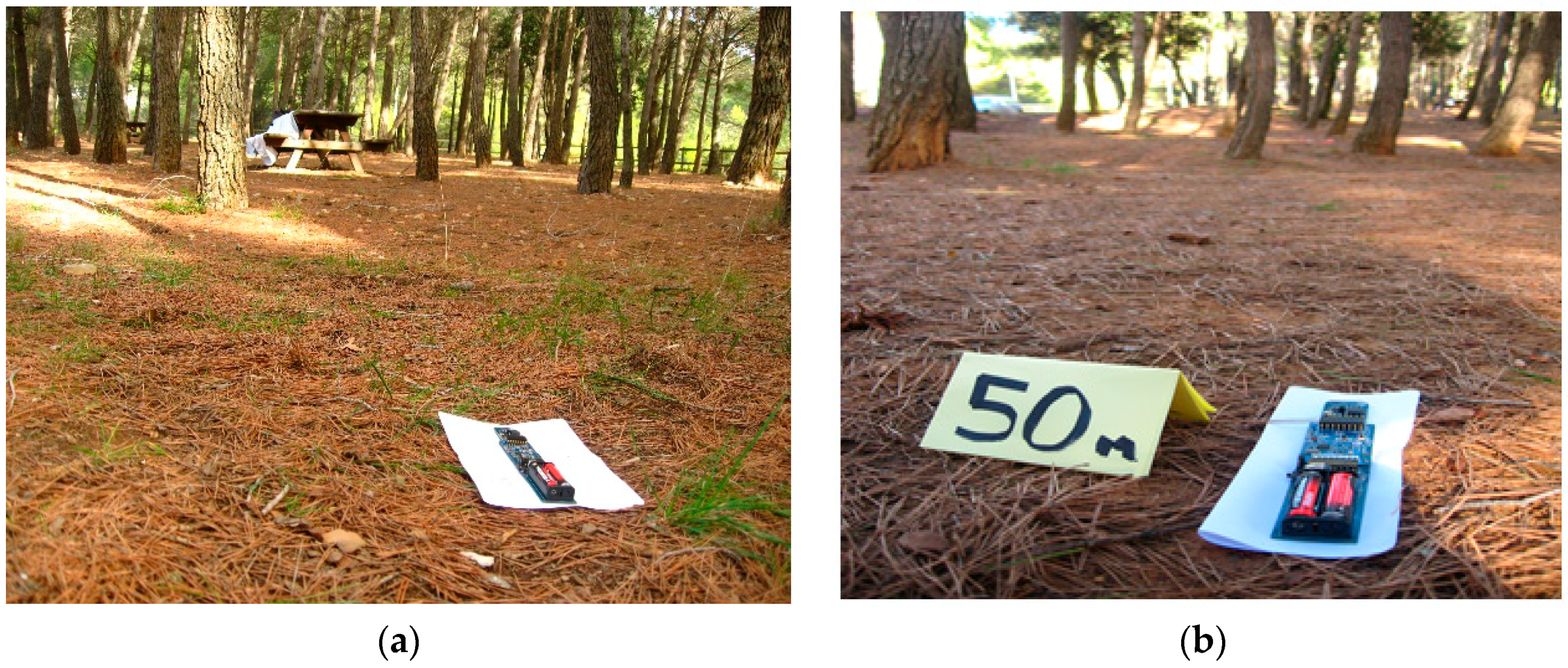
| Plain forest | 51 ± 5 | Pine forest area with scrubland |
| Plain forest | 80 ± 5 | Zone of pine forest with scrubland. BS at 1 m height |
| Irregular forest | 35 ± 5 | Pine forest area with slopes |
| Irregular forest | 45 ± 5 | Pine forest area with slopes. BS at 1 m height |
| Flat agricultural land | 120 ± 10 | Plot of ploughed cereals. BS at 1 m height 1 |
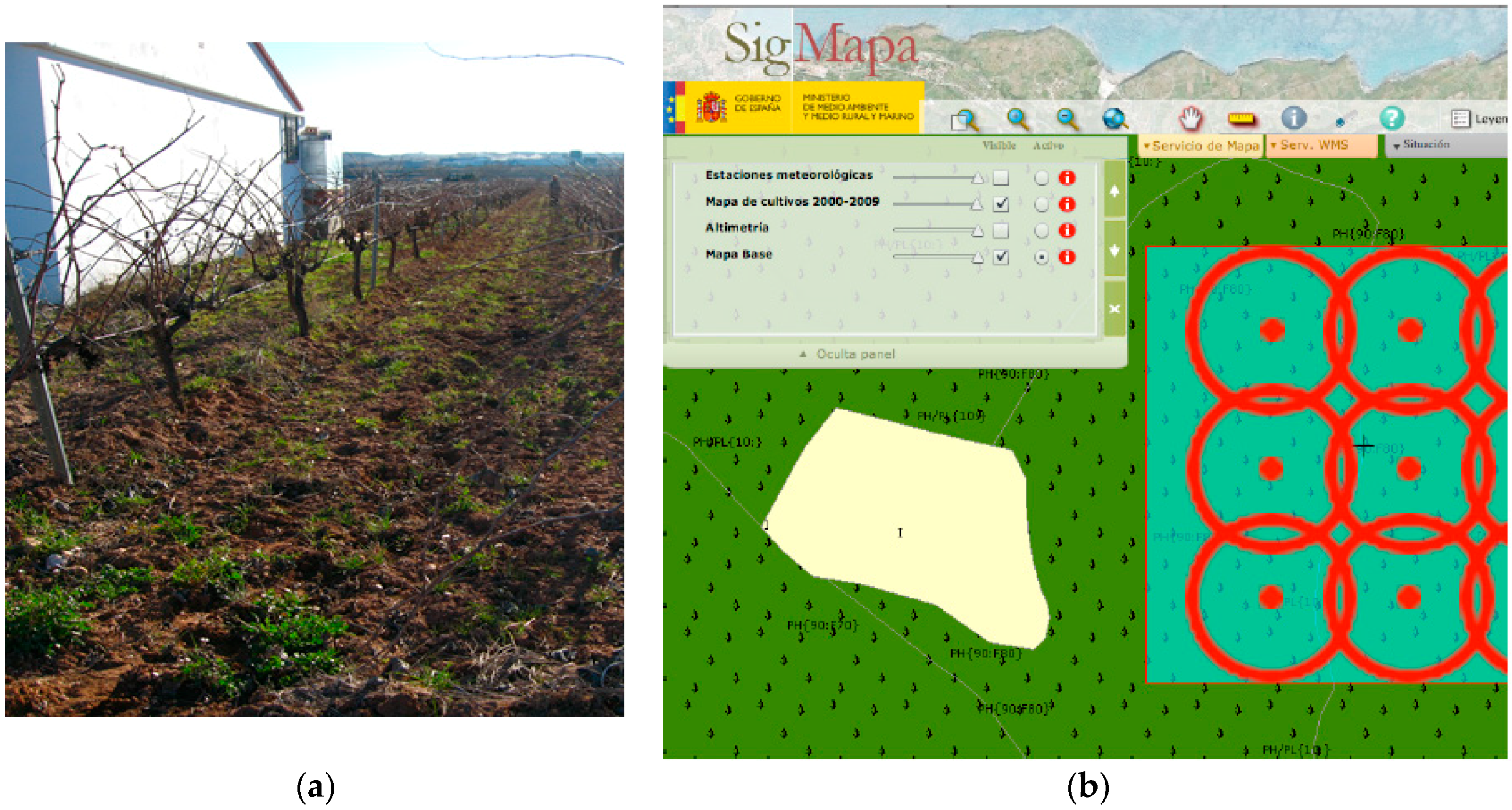
| Flat agricultural land | 70 ± 10 | Vineyard plot |
| Farmland | 85 ± 10 | Vineyard plot. BS at 1 m height |
| WSN | 5 × 5 | 6 × 6 | 7 × 7 | 8 × 8 |
|---|---|---|---|---|
| Max (G2D), (n) | 12.0 (n = 47) | 13.7 (n = 16) | 15.2 (n = 38) | 17.4 (n = 22) |
| Average (G2D) | 4.5 | 5.0 | 6.2 | 6.63 |
| 95% CI | [4.0, 5.0] | [4.4, 5.5] | [5.6, 6.8] | [5.9, 7.4] |
© 2018 by the authors. Licensee MDPI, Basel, Switzerland. This article is an open access article distributed under the terms and conditions of the Creative Commons Attribution (CC BY) license (http://creativecommons.org/licenses/by/4.0/).
Share and Cite
Navarro-Camba, E.A.; Felici-Castell, S.; Segura-García, J.; García-Pineda, M.; Pérez-Solano, J.J. Feasibility of a Stochastic Collaborative Beamforming for Long Range Communications in Wireless Sensor Networks. Electronics 2018, 7, 417. https://doi.org/10.3390/electronics7120417
Navarro-Camba EA, Felici-Castell S, Segura-García J, García-Pineda M, Pérez-Solano JJ. Feasibility of a Stochastic Collaborative Beamforming for Long Range Communications in Wireless Sensor Networks. Electronics. 2018; 7(12):417. https://doi.org/10.3390/electronics7120417
Chicago/Turabian StyleNavarro-Camba, Enrique A., Santiago Felici-Castell, Jaume Segura-García, Miguel García-Pineda, and Juan J. Pérez-Solano. 2018. "Feasibility of a Stochastic Collaborative Beamforming for Long Range Communications in Wireless Sensor Networks" Electronics 7, no. 12: 417. https://doi.org/10.3390/electronics7120417