Small Signal Stability of a Balanced Three-Phase AC Microgrid Using Harmonic Linearization: Parametric-Based Analysis

Abstract

The growth of power-electronic-based components is inescapable in future distribution grids (DGs). The introduction of these non-linear components poses many challenges, not only in terms of power quality, but also in terms of stability. These challenges become more acute when active loads are behaving as generators and power is flowing in reverse direction. The frequency-domain-based impedance modeling methods are preferred for small signal stability analysis (SSSA) of DGs involving such non-linear components. The harmonic linearization method can be used for impedance estimation, and afterwards, the Nyquist stability criterion can be used for stability analysis. In this paper, a parametric-based stability analysis of grid-connected active loads at the point of common coupling (PCC) is done by changing the parallel clustering distance and size of active loads. The results verify a positive impact on the stability of increasing parallel clustering and distance from the PCC and a negative impact of increasing the size of individual active loads.

1. Introduction

Electrical energy is the global source of energy, and every device in the future will eventually switch to the electric source of energy. It is necessary to not only utilize every possible resource of energy, but also make the transmission system as efficient, reliable, and stable as possible. The worldwide integration of renewables and other power electronic (PE)-based resources at distribution grids (DGs) is an effort to meet this ever-increasing energy demand [1,2,3].

The PE-based components, which are non-linear devices and draw/deliver constant power, have a dominant role in the future DGs [4,5,6,7]. It is expected from the PE-based active loads to give support to the grid under the IEEE-1547 grid integration code [8]. These PE-based non-linear devices behave as negative impedances and have a constant power nature, so traditional stability methods are unable to deal with these [9,10,11,12,13]. The growth and clustering of these new PE-based components at or near the point of common coupling (PCC) may lead to the instability of DGs [14,15,16,17,18,19].

In the frequency domain, the impedance-based modeling methods are used for small signal stability analysis (SSSA), where the impedances are estimated at the PCC to apply the stability criterion. Two frequency domain impedance-based SSSA modeling methods are harmonic linearization (HL) [20,21,22] and the impedance estimation method used for balanced three-phase system transformation into the synchronous reference frame (SRF) [23,24,25,26,27]. A comparative analysis for different stability analysis techniques is given in

Table 1. Comparative analysis of different stability techniques [20,28,29,30,31,32,33]. SRF, synchronous reference frame.

Model	Disadvantages	Reference
Lyapunov Methods (Time Domain)	A detailed system modeling is required for this method, so it does not work well for complex large systems. Its converter model is unable to capture the harmonic effect.	[28,29,31,33]
Probabilistic Methods (Time Domain)	It requires huge computational effort, so this method is very time consuming. Inaccurate first approximation may lead to faulty conclusions. Not all applied schemes work for complex large systems.	[32]
Phasor Model	It is often not differentiable due to significantly higher dimensions.	[20]
Bifurcation Theory	It is slow in the time domain and more complicated in the frequency domain for a higher order system.	[30]
SRF Method	Limited to only balanced three-phase systems.	[20,33]

.

In the SRF method, the balanced three-phase shunt current perturbation is used for impedance estimation [24,34,35,36] with the automated unit as presented in [36,37]. The impedance can be measured in real time with negligible additional cost [21,22,25,38,39,40,41,42,43] by this method. The limitation of the SRF method is that it can only be used to extract the impedances for balanced three-phase systems. This method is unable to capture harmonic effects. This method does not work for a system that is a combination of single- and a three-phase system. Furthermore, this method cannot be used for such a three-phase system in which one specific phase is heavily loaded as compared to the other phases or for an unbalanced system when a fault or other abnormal conditions occur [20,33]. In these scenarios, the zero-axis component is not zero, so the model cannot be linearized by using the SRF method to extract the impedances [20].

HL can be used without the limitations of SRF and is generally applicable to all kinds of AC systems. It can be used for a balanced three-phase system, a single-phase system, an unbalanced three-phase system having harmonics, and a three-phase system having one phase heavily loaded as compared to the other phases [20,33]. This method decomposes the AC system into linear and time-invariant symmetrical components without cross-coupling between them. Here, HL has many advantages over the other methods.

In this paper, the three-phase harmonic shunt-current-injection technique is used to introduce harmonic current perturbation at the PCC. The resultant harmonic voltage and harmonic current components on the source side and load side respectively are used to estimate the source and load side impedances by using the HL technique.

2. System Modeling Using HL

In this technique, the impedances of the non-linear system are extracted by superimposing a specific harmonic component. Superimposing a specific harmonic component involves two steps: firstly, harmonic perturbation is introduced into the system at the PCC, and secondly, the system response is monitored by using symmetrical components (positive, negative, and zero components).

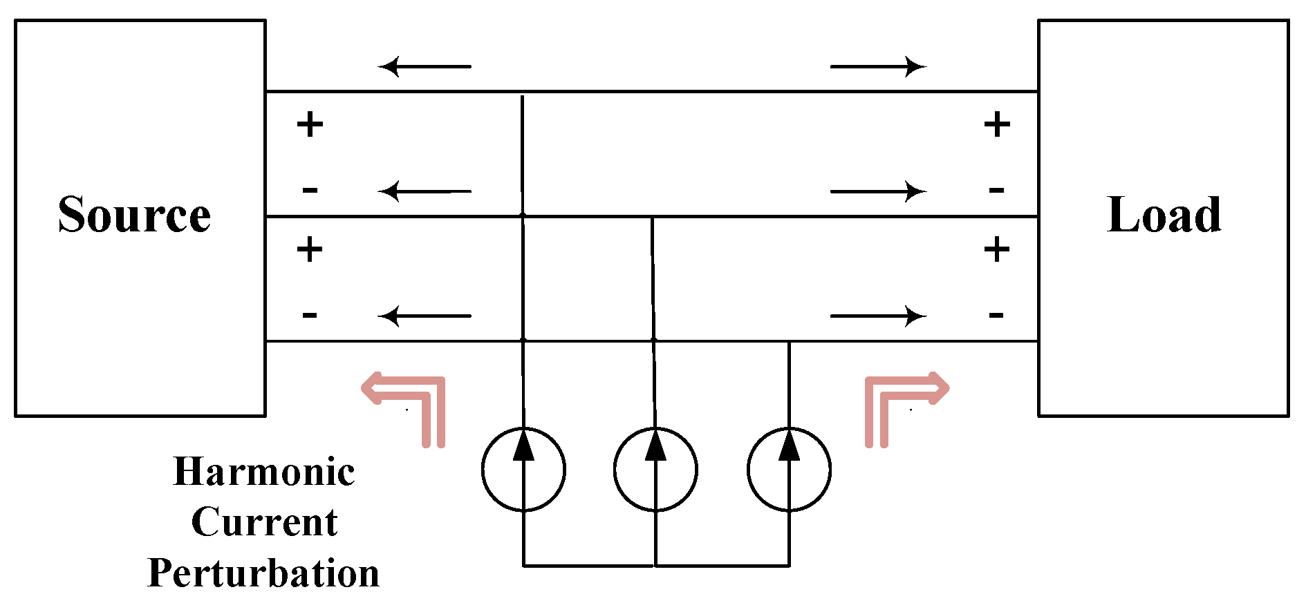
To estimate the impedances, the perturbation source is switched in at the PCC to inject the perturbations into the system. This perturbation source should have a perturbation magnitude significantly higher than the magnitude level PCC to have an impact at the PCC. Current perturbations are usually preferred because these are used in shunt configuration (as shown in Figure 1) as compared to voltage perturbations used in series configuration [24,34]. There are two basic methods, one based on electronic circuits and the other based on wound rotor induction machines, to switch in shunt current perturbations’ source for practical impedance estimation [34]. After injecting the perturbations at the PCC, the corresponding change in the source side and load side parameters (voltages and currents) is measured.

The Nyquist stability criterion (NSC) and/or Bode plot stability criteria are applied after developing the impedance-based model for the stability analysis in the frequency domain. Mostly, NSC is applied to verify the stability of the interconnected systems after extracting the impedances of both sides at the PCC.

The HL technique can deal with the positive and negative components of symmetrical components separately by using the property of linear time-invariant (LTI) systems. The system is stable only if all the components of the sequence domain are stable.

In the HL technique, specific harmonic perturbations are injected at a specific point, usually at the PCC. The old and new values of voltages and currents are measured both at the source side and load side. From the ratio of voltages and currents, the impedances are extracted from both the source and the load side.

This technique estimates the stability of the overall system at the PCC after extracting impedances through symmetrical components by developing a linear model (along a periodically time-varying operation trajectory) of the AC system having non-linear components. This operation trajectory may consist of any single harmonic or a collection of multiple odd harmonics for impedance extraction. The corresponding impedances in the sequence domain are extracted by using the harmonic balance principle [44] and small-signal approximation, assuming that the harmonic perturbation is sufficiently small.

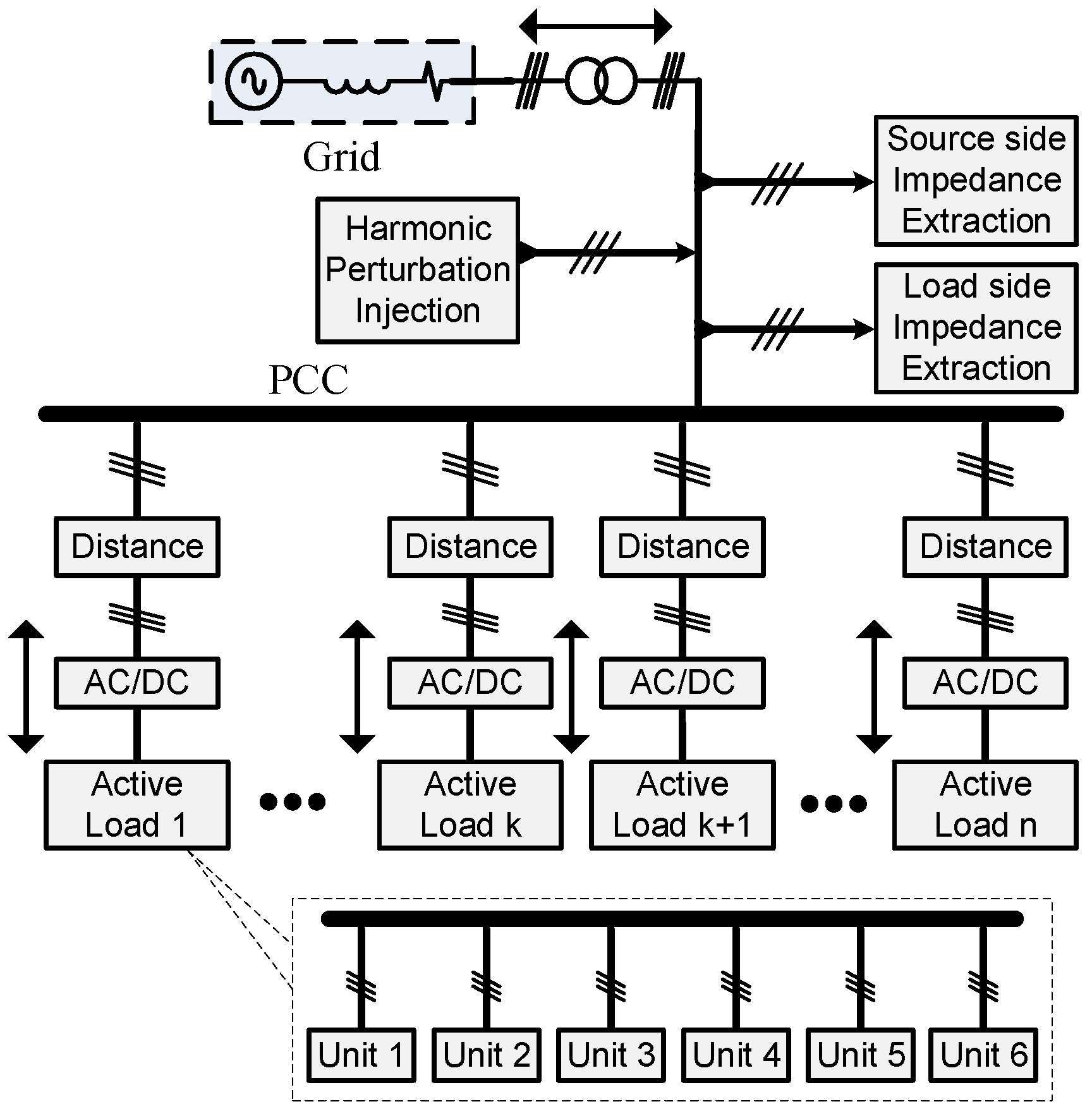
To ensure the power quality and grid stability, it is necessary that the grid interconnection of active loads be carefully examined. The objective of this work is to estimate and establish the pattern of small signal stability (SSS) in relation to the varying sizes, penetration level, and distances of the active loads from the PCC (as shown in Figure 2) to assess the stability of the distribution grid. Figure 2 describes how the size, distance, or penetration is changed for comparative stability analysis.

3. Mathematical Modeling of the Impedances at the PCC

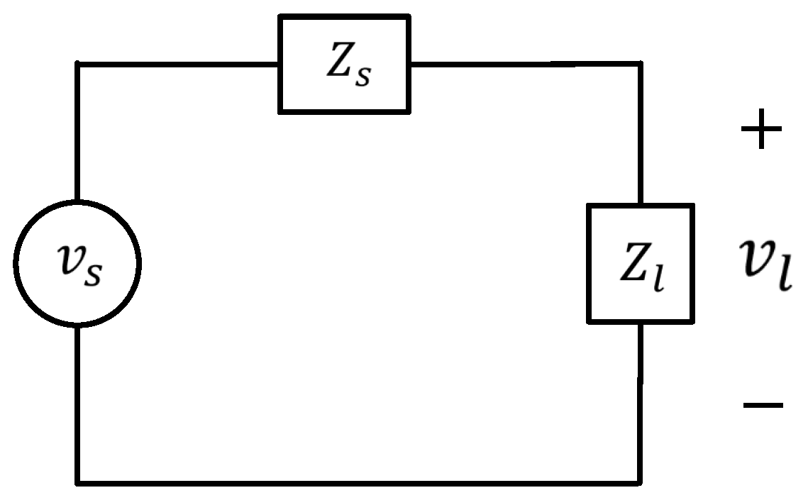
By applying the concept of the feedback control system on the simplified power system shown in Figure 3, the transfer function with $V_l\left(s\right)$ as output, $V_s\left(s\right)$ as input, $Z_1\left(s\right)$ as forward gain, and $Z_s\left(s\right)$ as reverse gain is given in (1).

$$\frac{\left[V_l\left(s\right)\right]}{\left[V_s\left(s\right)\right]}=\frac{1}{1+\left[Z_1\left(s\right)\right]{\left[Z_s\left(s\right)\right]}^{-1}}$$

(1)

The open loop gain, $L\left(s\right)$ can be extracted by rearranging (1) as given in (2).

$$V_l\left(s\right)={[1+\left[Z_1\left(s\right)\right]{\left[Z_s\left(s\right)\right]}^{-1}]}^{-1}\left[V_s\left(s\right)\right]$$

(2)

The stability can be determined by applying the NSC and only observing the Nyquist contour of the open loop transfer function, as given in (3).

$$L\left(s\right)=\left[Z_1\left(s\right)\right]{\left[Z_s\left(s\right)\right]}^{-1}$$

(3)

The transfer function of this power system can be determined in terms of input voltage $V_s$ and output voltage $V_l$, as shown in (4), where the term 012 (zero-positive-negative) represents that the quantities are in the HL.

$$\frac{V_{l\left(012\right)}\left(s\right)}{V_{s\left(012\right)}\left(s\right)}=\frac{1}{1+\left[Z_{l\left(012\right)}\left(s\right)\right]{\left[Z_{s\left(012\right)}\left(s\right)\right]}^{-1}}$$

(4)

This can be rearranged as given by (5) to extract the open loop gain $L\left(s\right)$ to apply the NSC on the open loop gain in (3).

$$V_{l\left(012\right)}\left(s\right)=\frac{V_{s\left(012\right)}\left(s\right)}{1+\left[Z_{l\left(012\right)}\left(s\right)\right]{\left[Z_{s\left(012\right)}\left(s\right)\right]}^{-1}}$$

(5)

Since the HL technique uses the symmetrical components for stability analysis, therefore relations are expressed in terms of the symmetrical components.

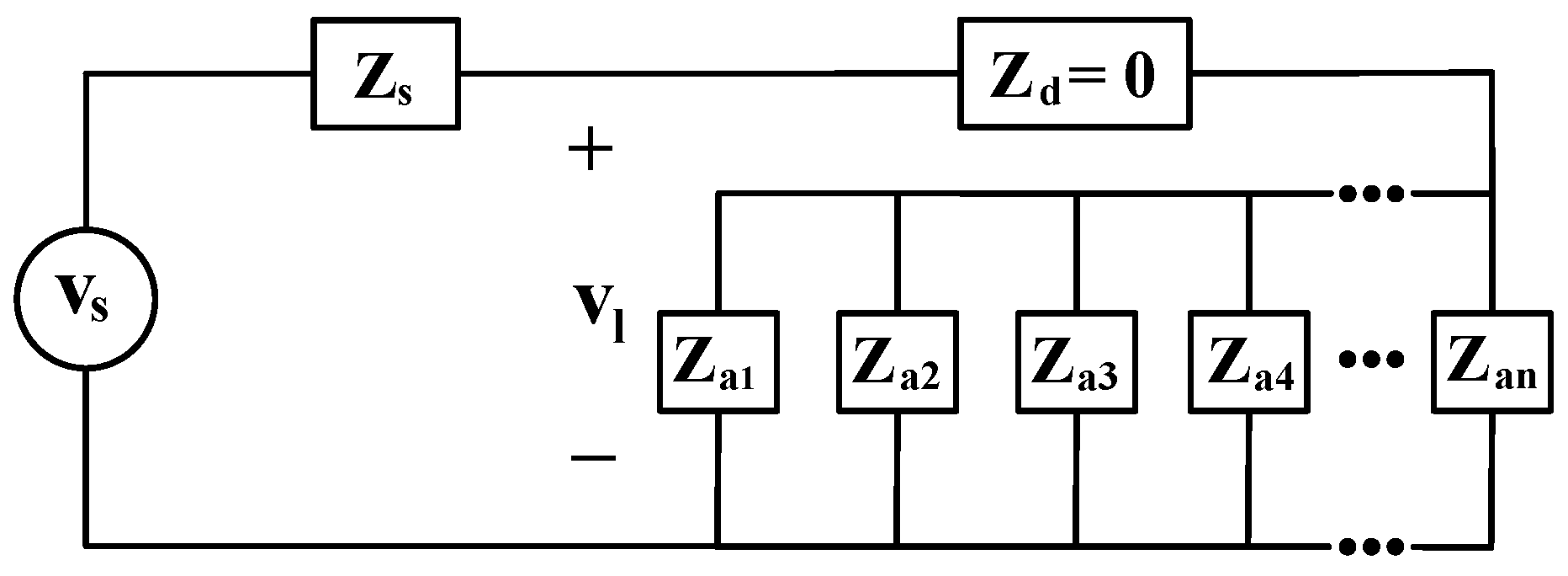
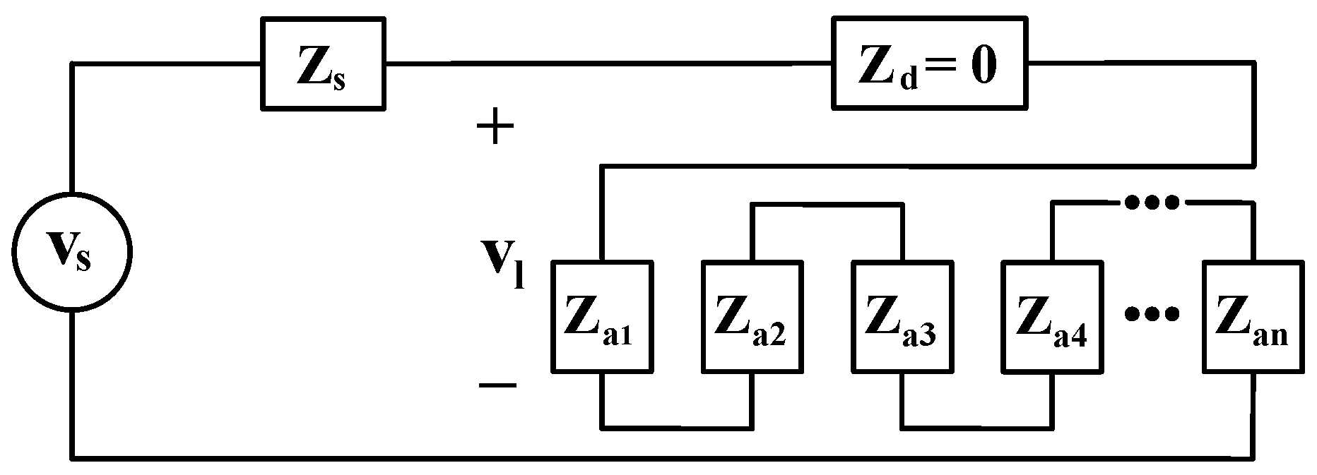
By increasing the parallel clustering of the active loads, at a specific frequency, the effective value of the load side impedance decreases at the PCC as shown in Figure 4 and as given by (6), where $Z_a$ is the impedance of non-linear active loads connected at the PCC.

$$\frac{1}{Z_a}=\frac{1}{Z_{a1}}+\frac{1}{Z_{a2}}+\frac{1}{Z_{a3}}+\frac{1}{Z_{a4}}+\dots +\frac{1}{Z_{an}}$$

(6)

The total load side impedance $Z_l$ can be expressed as given by (7).

$$Z_l=Z_d+Z_a$$

(7)

On the other hand, by increasing serial clustering (size) at the PCC, at a specific frequency, the effective value of load side impedance $Z_l$ increases, as shown in Figure 5 and as given by (8).

$$Z_l=Z_{a1}+Z_{a2}+Z_{a3}+Z_{a4}+\dots +Z_{an}+Z_d$$

(8)

If (8) is compared with (7), it is clear that the value of $Z_a=Z_{a1}+Z_{a2}+Z_{a3}+Z_{a4}+\dots +Z_{an}$ is increasing with size while $Z_d$ remains constant.

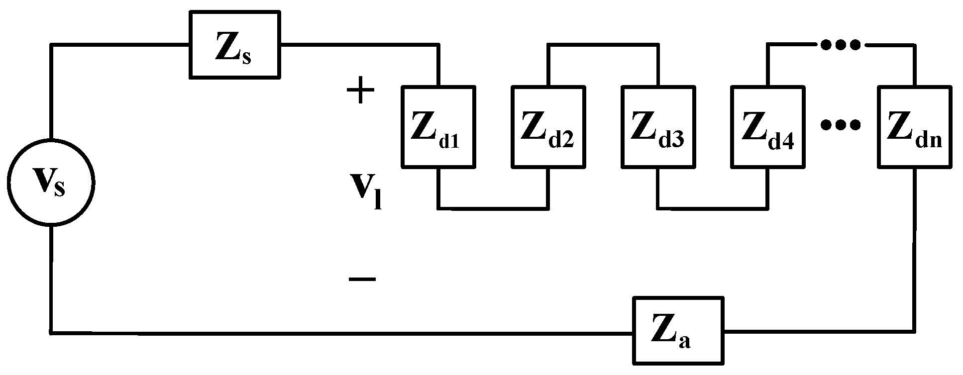
Finally, by increasing the distance from the PCC, at a specific frequency, the effective value of the load side impedance $Z_l$ decreases. This is because as the distance increases, the contribution of non-linear active load impedance in total series impedance decreases, as shown in Figure 6 and as given by (9).

$$Z_l=Z_{d1}+Z_{d2}+Z_{d3}+Z_{d4}+\dots +Z_{dn}+Z_a$$

(9)

If (9) is compared with (7), it is clear that the value of $Z_d=Z_{d1}+Z_{d2}+Z_{d3}+Z_{d4}+\dots +Z_{dn}$ is increasing with distance, while $Z_a$ remains constant.

In the impedance-based method, the perturbations are injected into the distribution system with the perturbation injection point dividing the system into two parts. The part with larger AC sources is called the source side, and the other part is called the load side.

The first step to determine the impedance is to superimpose the harmonic perturbation over the fundamental carrier signal. Then, the second step is to determine the resultant change in the response of that specific harmonic component at the frequency of interest. The fundamental or any other single harmonic, as well as multiple harmonics can be superimposed on the original power wave to extract the impedances. The current perturbations are injected into the system in shunt, as shown in Figure 1. Three-phase AC voltage and current are converted into symmetrical components at the point of injection. The source and load impedances are then extracted using the ratio of voltage and current at the extraction point. The impedance extracted from the ratio of symmetrical components of voltage and currents can be directly used for stability analysis. A typical impedance measurement setup is shown in Figure 7.

The load and source side impedance matrix in symmetrical components are given by (10) and (11):

$${\left[\begin{array}{c}{Z}_{l\left(012\right)}\end{array}\right]}_{3\times 3}=\left[\begin{array}{ccc}{Z}_{l\left(00\right)}& Z_{l\left(01\right)}& Z_{l\left(02\right)}\\ Z_{l\left(10\right)}& Z_{l\left(11\right)}& Z_{l\left(12\right)}\\ Z_{l\left(20\right)}& Z_{l\left(21\right)}& Z_{l\left(22\right)}\end{array}\right]$$

(10)

$${\left[\begin{array}{c}{Z}_{s\left(012\right)}\end{array}\right]}_{3\times 3}=\left[\begin{array}{ccc}{Z}_{s\left(00\right)}& Z_{s\left(01\right)}& Z_{s\left(02\right)}\\ Z_{s\left(10\right)}& Z_{s\left(11\right)}& Z_{s\left(12\right)}\\ Z_{s\left(20\right)}& Z_{s\left(21\right)}& Z_{s\left(22\right)}\end{array}\right]$$

(11)

The relation between voltage and current in symmetrical components on the load side is given by (12) for a balanced three-phase system.

$${\left[\begin{array}{c}{V}_{l\left(012\right)}\end{array}\right]}_{3\times 1}={\left[\begin{array}{c}{Z}_{l\left(012\right)}\end{array}\right]}_{3\times 3}{\left[\begin{array}{c}{I}_{l\left(012\right)}\end{array}\right]}_{3\times 1}$$

(12)

The perturbations are introduced at the PCC to build nine full equations based on a 3 × 3 impedance matrix for both the source side and the load side. A single perturbation can generate only three equations (for both the source and load side) [45]. At least three perturbations are introduced to build full 3 × 3 impedance matrices for the source and the load side. Voltages on the load side in HL after first perturbation are given by (13):

$${\left[\begin{array}{c}{V}_{l\left(012\right)}^1\end{array}\right]}_{3\times 1}={\left[\begin{array}{c}{Z}_{l\left(012\right)}\end{array}\right]}_{3\times 3}{\left[\begin{array}{c}{I}_{l\left(012\right)}^1\end{array}\right]}_{3\times 1}$$

(13)

The voltages in HL on the load side after the second perturbation are given by (14):

$${\left[\begin{array}{c}{V}_{l\left(012\right)}^2\end{array}\right]}_{3\times 1}={\left[\begin{array}{c}{Z}_{l\left(012\right)}\end{array}\right]}_{3\times 3}{\left[\begin{array}{c}{I}_{l\left(012\right)}^2\end{array}\right]}_{3\times 1}$$

(14)

The voltages in HL on the load side after the third perturbation are given by (15):

$${\left[\begin{array}{c}{V}_{l\left(012\right)}^3\end{array}\right]}_{3\times 1}={\left[\begin{array}{c}{Z}_{l\left(012\right)}\end{array}\right]}_{3\times 3}{\left[\begin{array}{c}{I}_{l\left(012\right)}^3\end{array}\right]}_{3\times 1}$$

(15)

Equations (13)–(15) can be written in combined form as (16).

$${\left[\begin{array}{c}{V}_{l\left(012\right)}\end{array}\right]}_{3\times 3}={\left[\begin{array}{c}{Z}_{l\left(012\right)}\end{array}\right]}_{3\times 3}{\left[\begin{array}{c}{I}_{l\left(012\right)}\end{array}\right]}_{3\times 3}$$

(16)

Rearranging (16) results in (17),

$${\left[\begin{array}{c}{Z}_{l\left(012\right)}\end{array}\right]}_{3\times 3}={\left[\begin{array}{c}{V}_{l\left(012\right)}\end{array}\right]}_{3\times 3}{\left[\begin{array}{c}{I}_{l\left(012\right)}\end{array}\right]}_{3\times 3}^{-1}$$

(17)

Similarly, for the source side, (17) can be rewritten as (18):

$${\left[\begin{array}{c}{Z}_{s\left(012\right)}\end{array}\right]}_{3\times 3}={\left[\begin{array}{c}{V}_{s\left(012\right)}\end{array}\right]}_{3\times 3}{\left[\begin{array}{c}{I}_{s\left(012\right)}\end{array}\right]}_{3\times 3}^{-1}$$

(18)

The unknown impedances can be found through simulation or the experiment-based impedance method.

4. Simulation Results

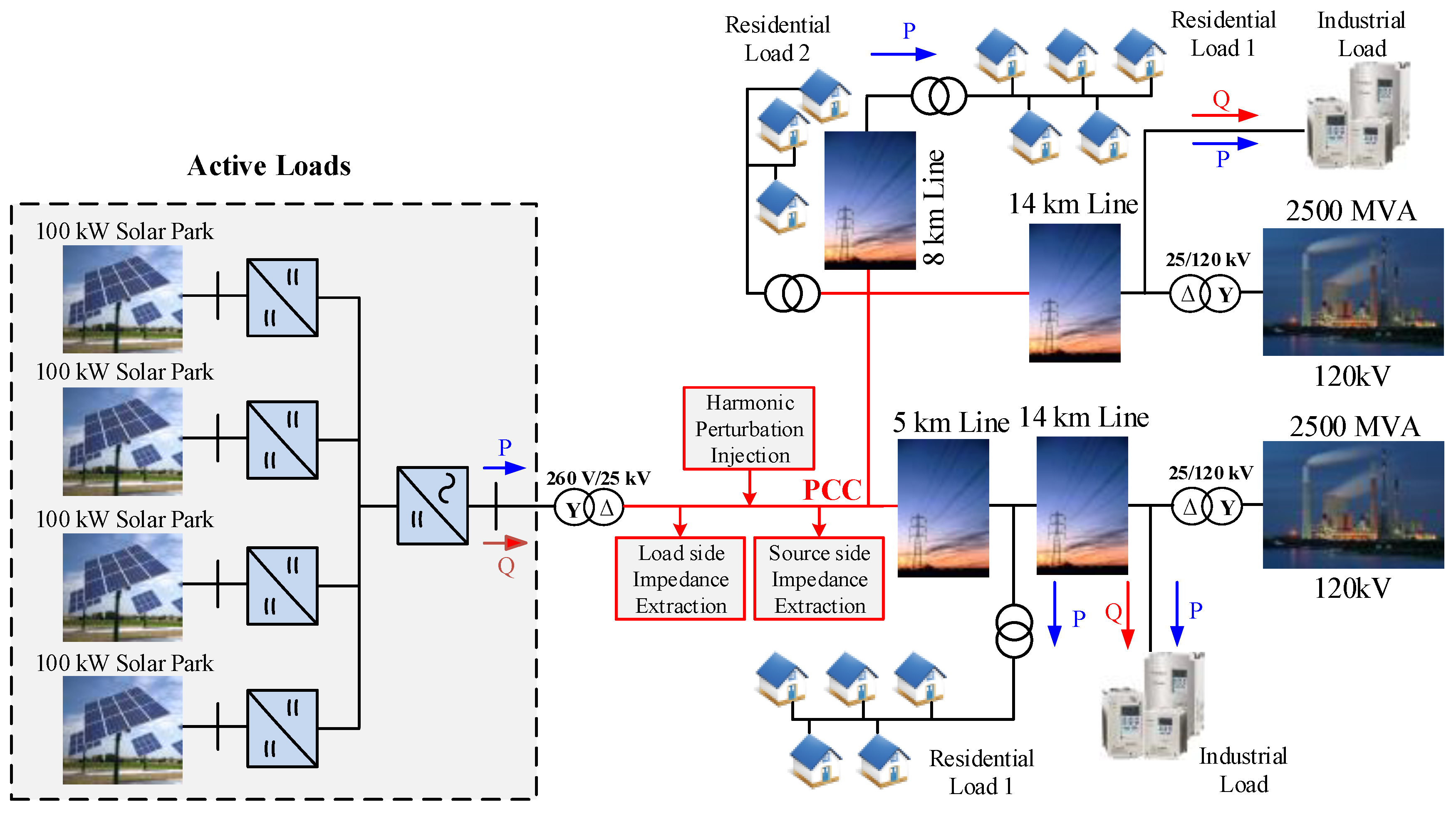
The Simulink model of the grid-connected PV systems (shown in Figure 8) was used for stability analysis.

The detail of the system parameters is tabulated in

Table 2. Parameters at the PCC for different penetrations of active loads.

Parameter	Symbol	Value	Symbol	Value
Power Source	P	2500 MVA	V	120 kV
Line Section	$R\left[r_1\right]$	[0.1153]	$L\left[r_1\right]$	$[1.05\times {10}^{-3}]$
Line Section	$R\left[r_0\right]$	[0.413]	$L\left[r_0\right]$	$[3.32\times {10}^{-3}]$
Industrial Load	P	30 MW	Q	2 MVar
Residential Load 1	P	2 MW	Q	0
Residential Load 2	P	100 kW	Q	0

. In this model, different PV systems, each having a rating of 100 kW, were integrated with PCC. In this configuration, each unit of the PV system consisted of 100 kW, and the size of the active load may consist of multiple units. To achieve the objective of comparative analysis, it was assumed that all the PV systems were working at the same temperature and receiving the same amount of irradiance. The stability at the PCC was evaluated against three different indices. These three indices were;

• First, stability was assessed by changing the parallel clustering (penetration) of grid-connected active loads.
• Then, the stability was evaluated by changing the distance of active loads from the PCC.
• Afterwards, the stability at the PCC was assessed by changing the serial clustering (size) of active loads.

These parameters were changed one by one, and the corresponding change in load side impedance at the PCC was recorded. Then, NSC was applied on the load side and source side impedance in each of the above cases. The corresponding Nyquist plots were drawn against different specific values of these parameters. The objective was to assess how varying these parameter affected the stability at the PCC.

The dynamic models of grid-connected active loads were developed and designed in MATLAB Simulink. The block diagram of the grid-connected active loads is shown in Figure 2 where PCC was working at a 25-kV voltage rating. Figure 2 describes how the size, distance, or penetration was changed for comparative stability analysis.

4.1. Effect of Penetration

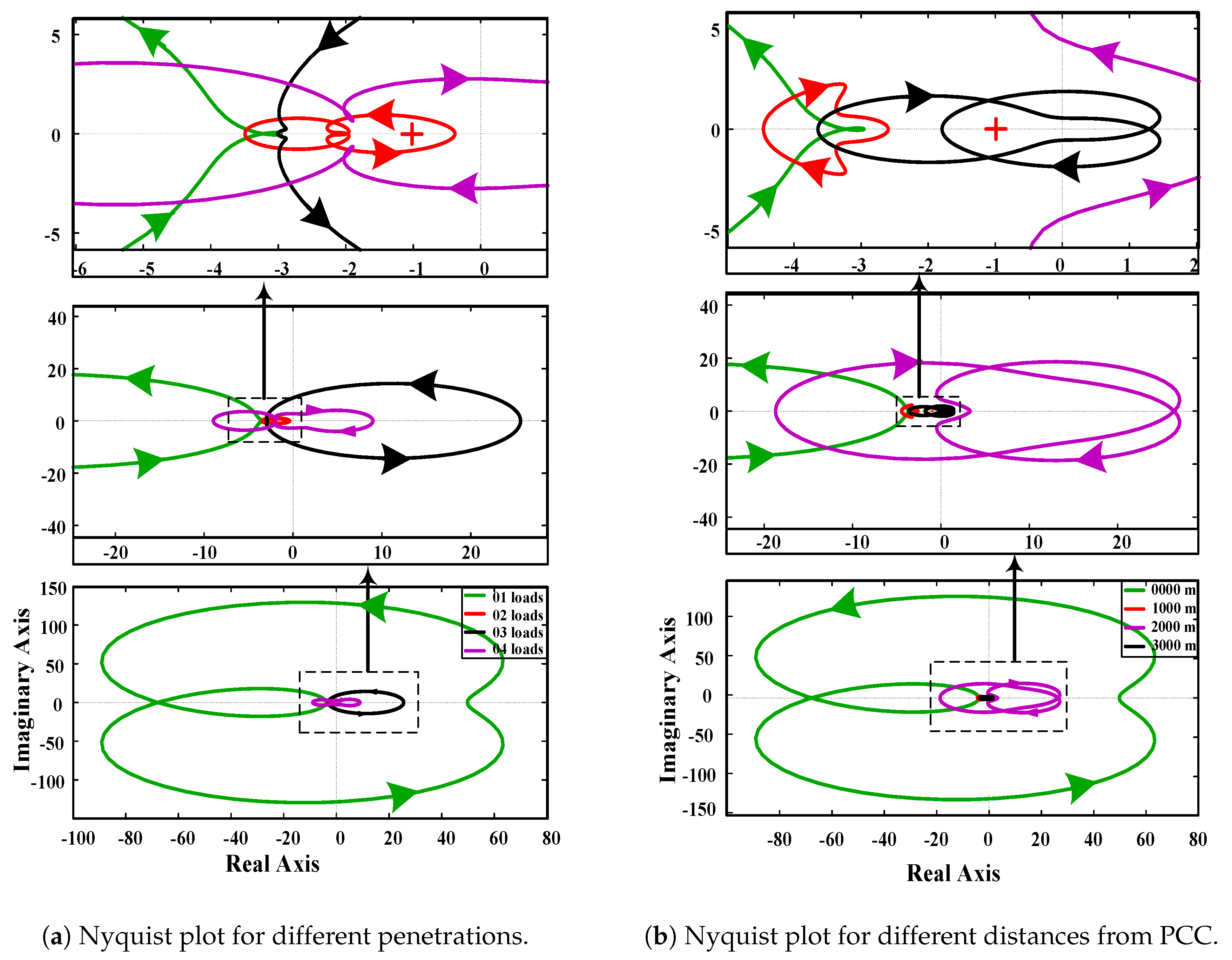
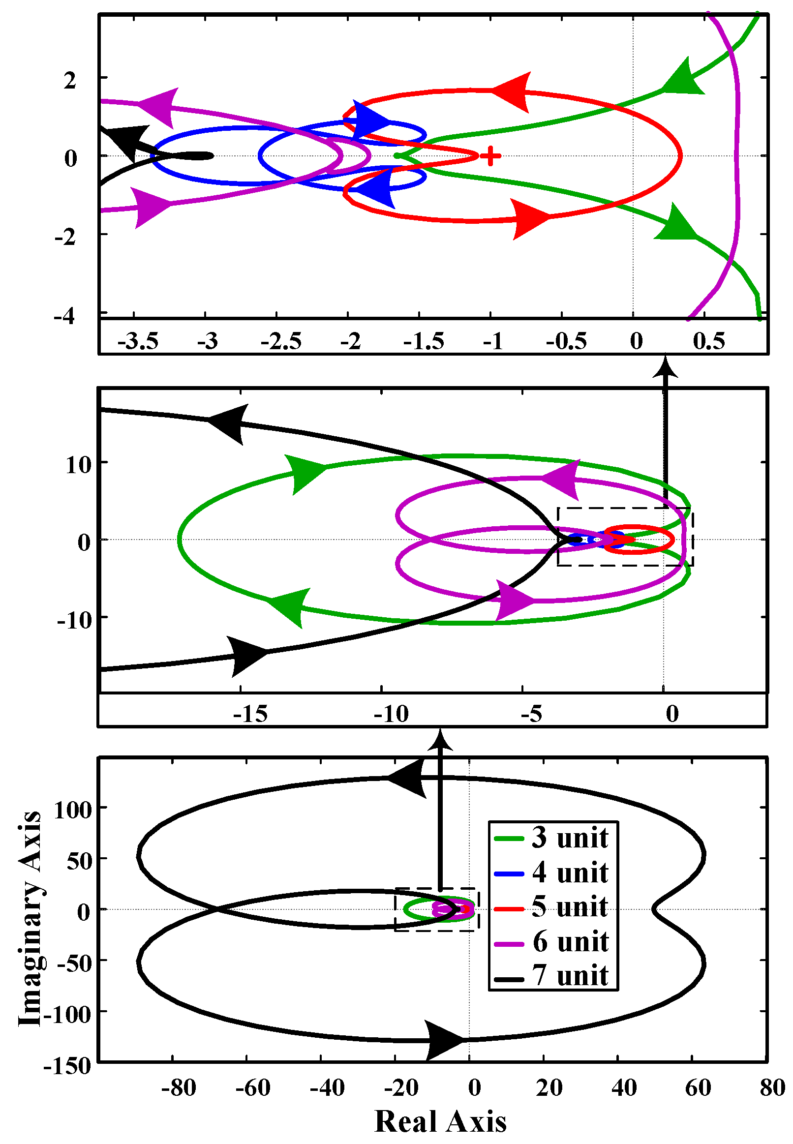
The first objective was to check the stability pattern at the PCC against various penetrations. The penetration of active loads was varied in a systematic way, and the corresponding change in load side impedance was recorded. The resultant Nyquist plots for different values of parallel clustering by keeping the distance and size constant are shown in a single plot in Figure 9a.

It is clear from these plots that as the parallel clustering increased, the anti-clockwise encirclements of −1 vanished. The anti-clockwise encirclements of −1 depicted the total number of closed loop poles in the night half plane, which caused the instability of the system. When the anti-clockwise encirclements of −1 vanished, the system became stable. The microgrid system was designed in such a way that the PCC was working at a stability boundary for different indices. Therefore, as the system indices were changed near the PCC, the system changed from unstable to stable or vice versa. Not all of the Nyquist plot is clearly visible to the naked eye, so the selected parts of the lower Nyquist plots are zoomed-in and shown above for better and clear understanding of the Nyquist plots. The system at the PCC was unstable when only a single active load (of size 700 kW i.e., seven units) was connected at the PCC (distance = 0 km). The Nyquist plot of one active load depicted an anti-clockwise encirclement, as shown in the lower part of Figure 9a. Similarly, the system at the PCC was still unstable when two and three active loads were connected respectively at the PCC in parallel configuration, as shown in the zoomed-in version of Figure 9a. When the parallel clustering reached the four active loads, keeping size and distance unchanged, the system at the PCC became stable. The stability would further improve by increasing the penetration at the PCC by keeping the distance and size constant.

4.2. Effect of Distance from PCC

To check the effect of the distance of active loads from the PCC to the stability at the PCC, the distance of active load was varied by keeping the penetration and size constant. The objective of selecting a specific penetration and a specific size was to keep the PCC near the stability boundary. The penetration of one active load and the size of seven units (700 kW) were chosen in this case. The load side impedance was recorded by changing the distance from the PCC by keeping the penetration and size constant in all the cases. The NSC was applied on the load and the source side impedances to get the Nyquist plot for different values of distances, as shown in Figure 9b.

The results show that the system was unstable at the PCC when the distance was 0 km because there was a pole in the right half plane (anti-clockwise encirclement of −1). As the distance was increased to 1 km, the anti-clockwise encirclement vanished (as shown in the zoomed-in version of the Nyquist plots), so the system became stable at the PCC. This stability further improved as the distance increased to 2 km and 3 km, respectively, by keeping the size and penetration constant.

4.3. Effect of the Sizes of Active Loads

To check the effect of changing the size of an active load on the stability at the PCC, the size was varied by keeping the distance and penetration constant. A single active load was connected at the PCC in this case, so the distance was 0 km and the penetration was one active load. The load side impedance changed by changing the size. Different Nyquist plots were obtained when NSC was applied on different values of load side impedances and the same value of source side impedance. These Nyquist plots, each corresponding to different sizes of an active load, are shown in Figure 10.

Initially, the system was stable at the PCC, as there were no anti-clockwise encirclements of −1, which depicts that there were no poles in the right half plane. The system remained stable when the size of active loads was equal to or less than four units (400 kW). As the size of the system reached five units (500 kW), the system became unstable, and there was an anti-clockwise encirclement of −1, which depicts a pole in the right half plane. The stability further deteriorated as the size was increased further.

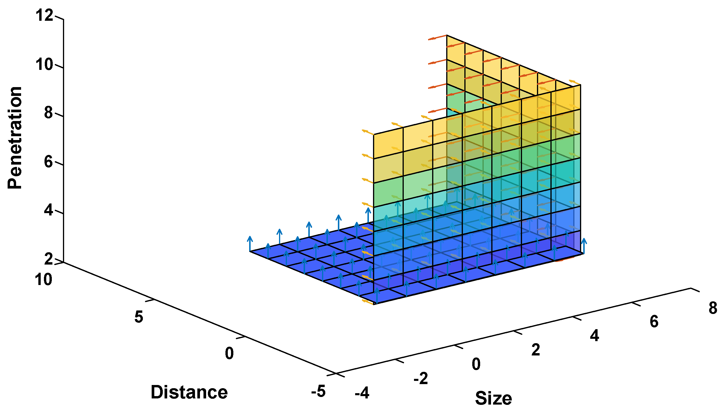
The summery of the above three cases is given in

Table 3. Effect of different parameters on stability.

Penetration	Distance at PCC	Size	Effect on Stability
Increasing	Constant	Constant	Improve
Constant	Increasing	Constant	Improve
Constant	Constant	Increasing	Deteriorate

. According to this table, when the size was increased by keeping other parameters constant, the stability at the PCC deteriorated. When the distance was increased from the PCC by keeping other parameters constant, the stability at the PCC improved.

When the penetration was increased at the PCC by keeping the distance and size constant, the stability at the PCC improved. The stability behavior at the PCC by changing the size, distance, and penetration is given in Figure 11. Figure 11 depicts the stability region in connection with size, distance, and penetration. Firstly, keeping distance (=0 km) and penetration (=1) constant, the instability boundary for size was six units. As the size decreased, the stability improved. The direction of the arrow shows the stability behavior (from the unstable to stable region and from the stable to more stable region). Secondly, keeping distance (=0 km) and size (=7 units) constant, the instability boundary for penetration was one active load. The direction of the arrow shows the stability behavior, so as the penetration increased, the stability improved further. Finally, keeping size (=7 units) and penetration (=1) constant, the instability boundary for distance was 0 km. As the distance increased, the stability improved further. These results verified that there was a strong relation between these parameters and the stability at the PCC. Changing any other system components, the stability boundary would shift, but the behavior of the stability and the relation to these parameters will remain the same.

The simulation results presented were near the stability boundary. These results and stability boundaries were only specific for the system designed for simulation. Changing the system would change the stability boundary because impedance would change. However, the relation of different parameters with the Nyquist stability would remain the same.

5. Conclusions

In this paper, the SSSA at the PCC was done by varying one of three parameters (size distance and penetration) and keeping the other two constant. The results show that the stability pattern of NSC changes in a systematic way in response to a systematic change in any of these parameters. The impact of increasing penetration and increasing distance from the PCC was positive on the stability at the PCC, while the impact of increasing the size (while keeping the other parameters constant) was negative on the stability at the PCC. Thus, a change in any of these parameters will play a significant role in deciding the stability at the PCC.

The design and composition, as well as the distance from the PCC of active loads play an important role in the SSS of an AC microgrid. These parameters must be thoroughly assessed before deploying active loads at the PCC.

References

- Siddique, M.N.; Ahmad, A.; Nawaz, M.K.; Bukhari, S.B.A. Optimal integration of hybrid (wind-solar) system with diesel power plant using HOMER. Turk. J. Electr. Eng. Comput. Sci. 2015, 23, 1547–1557. [Google Scholar] [CrossRef]
- Matos, E.O.D.; Soares, T.M.; Bezerra, U.H.; De Tostes, L.M.E.; Rodrigo, A.; Manito, A.; Cordeiro, B.C., Jr. Using linear and non-parametric regression models to describe the contribution of non-linear loads on the voltage harmonic distortions in the electrical grid. IET Gener. Transm. Distrib. 2016, 10, 1825–1832. [Google Scholar] [CrossRef]
- Li, Y.W.; He, J. Distribution System Harmonic Compensation Methods: An Overview of DG-Interfacing Inverters. IEEE Ind. Electron. Mag. 2014, 8, 18–31. [Google Scholar] [CrossRef]
- Bhattacharyya, S.; Cobben, S.; Ribeiro, P.; Kling, W. Harmonic emission limits and responsibilities at a point of connection. IET Gener. Transm. Distrib. 2012, 6, 256–264. [Google Scholar] [CrossRef]
- Wildrick, C.; Lee, F.; Cho, B.; Choi, B. A method of defining the load impedance specification for a stable distributed power system. In Proceedings of the IEEE Power Electronics Specialist Conference PESC ’93, Seattle, WA, USA, 20–24 June 1993; pp. 826–832. [Google Scholar]
- Khaligh, A.; Rahimi, A.; Emadi, A. Negative Impedance Stabilizing Pulse Adjustment Control Technique for DC/DC Converters Operating in Discontinuous Conduction Mode and Driving Constant Power Loads. IEEE Trans. Veh. Technol. 2007, 56, 2005–2016. [Google Scholar] [CrossRef]
- Emadi, A.; Ehsani, M. Negative impedance stabilizing controls for pwm Dc-Dc converters using feedback linearization techniques. In Proceedings of the 35th Intersociety Energy Conversion Engineering Conference and Exhibit (Cat. No.00CH37022), Las Vegas, NV, USA, 24–28 July 2000; Volume 1, pp. 613–620. [Google Scholar]
- Preda, T.; Uhlen, K.; Nordgård, D.E. An overview of the present grid codes for integration of distributed generation. In Proceedings of the CIRED 2012 Workshop: Integration of Renewables into the Distribution Grid, Lisbon, Portugal, 29–30 May 2012; pp. 1–4. [Google Scholar]
- Sudhoff, S.; Corzine, K.; Glover, S.; Hegner, H.; Robey, H. DC link stabilized field oriented control of electric propulsion systems. IEEE Trans. Energy Convers. 1998, 13, 27–33. [Google Scholar] [CrossRef]
- Emadi, A.; Khaligh, A.; Rivetta, C.; Williamson, G. Constant Power Loads and Negative Impedance Instability in Automotive Systems: Definition, Modeling, Stability, and Control of Power Electronic Converters and Motor Drives. IEEE Trans. Veh. Technol. 2006, 55, 1112–1125. [Google Scholar] [CrossRef]
- Feng, X.; Liu, J.; Lee, F. Impedance Specifications for Stable DC Distributed Power Systems. IEEE Trans. Power Electron. 2002, 17, 157–162. [Google Scholar] [CrossRef]
- Belkhayat, M.; Cooley, R.; Witulski, A. Large Signal Stability Criteria For Distributed Systems with Constant Power Loads. In Proceedings of the PESC ’95 - Power Electronics Specialist Conference, Atlanta, GA, USA, 18–22 June 1995; pp. 1333–1338. [Google Scholar]
- Liserre, M.; Teodorescu, R.; Blaabjerg, F. Stability of photovoltaic and wind turbine grid-connected inverters for a large set of grid impedance values. IEEE Trans. Power Electron. 2006, 21, 263–272. [Google Scholar] [CrossRef]
- Liu, J.; Feng, X.; Lee, F.; Borojevich, D. Stability margin monitoring for DC distributed power systems via current/voltage perturbation. In Proceedings of the Sixteenth Annual IEEE Applied Power Electronics Conference and Exposition APEC 2001 (Cat. No.01CH37181), Anaheim, CA, USA, 4–8 March 2001; Volume 2, pp. 745–751. [Google Scholar]
- Grigore, V.; Hatonen, J.; Kyyra, J.; Suntio, T. Dynamics of a buck converter with a constant power load. In Proceedings of the PESC 98 Record. 29th Annual IEEE Power Electronics Specialists Conference (Cat. No.98CH36196), Fukuoka, Japan, 22 May 1998; Volume 1, pp. 72–78. [Google Scholar]
- Chen, M.; Sun, J. Low-Frequency Input Impedance Modeling of Boost Single-Phase PFC Converters. IEEE Trans. Power Electron. 2007, 22, 1402–1409. [Google Scholar] [CrossRef]
- Prodic, A. Compensator Design and Stability Assessment for Fast Voltage Loops of Power Factor Correction Rectifiers. IEEE Trans. Power Electron. 2007, 22, 1719–1730. [Google Scholar] [CrossRef]
- Mithulananthan, N.; Kumar Saha, T.; Chidurala, A. Harmonic impact of high penetration photovoltaic system on unbalanced distribution networks—Learning from an urban photovoltaic network. IET Renew. Power Gener. 2016, 10, 485–494. [Google Scholar]
- He, J.; Li, Y.W.; Munir, M.S. A Flexible Harmonic Control Approach Through Voltage-Controlled DG-Grid Interfacing Converters. IEEE Trans. Ind. Electron. 2012, 59, 444–455. [Google Scholar] [CrossRef]
- Sun, J. Small-signal methods for AC distributed power systems—A review. IEEE Trans. Power Electron. 2009, 24, 2545–2554. [Google Scholar]
- Cespedes, M.; Sun, J. Adaptive Control of Grid-Connected Inverters Based on Online Grid Impedance Measurements. IEEE Trans. Sustain. Energy 2014, 5, 516–523. [Google Scholar] [CrossRef]
- Roinila, T.; Vilkko, M.; Sun, J. Online Grid Impedance Measurement Using Discrete-Interval Binary Sequence Injection. IEEE J. Emerg. Sel. Top. Power Electron. 2014, 2, 985–993. [Google Scholar] [CrossRef]
- Belkhayat, M. Stability Criteria for AC Power Systems with Regulated Loads. Ph.D. Thesis, Purdue University, West Lafayette, IN, USA, 1997. [Google Scholar]
- Francis, G.; Burgos, R.; Boroyevich, D.; Wang, F.; Karimi, K. An Algorithm and Implementation System for Measuring Impedance in the D-Q Domain. In Proceedings of the 2011 IEEE Energy Conversion Congress and Exposition, Phoenix, AZ, USA, 17–22 September 2011; pp. 3221–3228. [Google Scholar]
- Wen, B.; Dong, D.; Boroyevich, D.; Burgos, R.; Mattavelli, P.; Shen, Z. Impedance-Based Analysis of Grid-Synchronization Stability for Three-Phase Paralleled Converters. IEEE Trans. Power Electron. 2016, 31, 26–38. [Google Scholar] [CrossRef]
- Valdivia, V.; Lazaro, A.; Barrado, A.; Zumel, P.; Fernandez, C.; Sanz, M. Black-Box Modeling of Three-Phase Voltage Source Inverters for System-Level Analysis. IEEE Trans. Ind. Electron. 2012, 59, 3648–3662. [Google Scholar] [CrossRef]
- Rygg, A.; Molinas, M.; Zhang, C.; Cai, X. A Modified Sequence-Domain Impedance Definition and Its Equivalence to the dq-Domain Impedance Definition for the Stability Analysis of AC Power Electronic Systems. IEEE J. Emerg. Sel. Top. Power Electron. 2016, 4, 1383–1396. [Google Scholar] [CrossRef] [Green Version]
- Kundur, P. Power System Stability and Control; McGraw-Hill: New York, NY, USA, 1994. [Google Scholar]
- Yao, Z.; Therond, P.G.; Davat, B. Stability analysis of power systems by the generalised nyquist criterion. In Proceedings of the 1994 International Conference on Control Control ’94, Coventry, UK, 21–24 March 1994; pp. 739–744. [Google Scholar]
- Guanrong, C.; Moiola, J.L. Hopf Bifurcation Analysis: A Frequency Domain Approach; World Scientific: Singapore, 1996. [Google Scholar]
- Sanchez, S. Stability Investigation of Power Electronics Systems: A Microgrid Case. Ph.D. Thesis, Norwegian University of Science and Technology, Trondheim, Norway, 2015. [Google Scholar]
- Xu, Q.; Member, S.; Ma, F.; Luo, A.; Member, S. Analysis and Control of M3C based UPQC for Power Quality Improvement in Medium/High Voltage Power Grid. IEEE Trans. Power Electron. 2016, 31, 8182–8194. [Google Scholar] [CrossRef]
- Amin, M.; Molinas, M. Small-Signal Stability Assessment of Power Electronics based Power Systems: A Discussion of Impedance and Eigenvalue-based Methods. IEEE Trans. Ind. Appl. 2017, 53, 5014–5030. [Google Scholar] [CrossRef]
- Familiant, Y.A.; Huang, J.; Corzine, K.A.; Belkhayat, M. New Techniques for Measuring Impedance Characteristics of Three-Phase AC Power Systems. IEEE Trans. Power Electron. 2009, 24, 1802–1810. [Google Scholar] [CrossRef]
- Valdivia, V.; Lázaro, A.; Barrado, A.; Zumel, P.; Fernández, C.; Sanz, M. Impedance Identification Procedure of Three-Phase Balanced Voltage Source Inverters Based on Transient Response Measurements. IEEE Trans. Power Electron. 2011, 26, 3810–3816. [Google Scholar] [CrossRef]
- Shen, Z.; Jaksic, M.; Mattavelli, P.; Boroyevich, D.; Verhulst, J.; Belkhayat, M. Design and implementation of three-phase AC impedance measurement unit (IMU) with series and shunt injection. In Proceedings of the 2013 Twenty-Eighth Annual IEEE Applied Power Electronics Conference and Exposition (APEC), Long Beach, CA, USA, 17–21 March 2013; pp. 2674–2681. [Google Scholar]
- Shen, Z.; Jaksic, M.; Mattavelli, P.; Boroyevich, D.; Verhulst, J. Three-phase AC system impedance measurement unit (IMU) using chirp signal injection. In Proceedings of the 2013 Twenty-Eighth Annual IEEE Applied Power Electronics Conference and Exposition (APEC), Long Beach, CA, USA, 17–21 March 2013; pp. 2666–2673. [Google Scholar]
- Wen, B.; Boroyevich, D.; Burgos, R.; Mattavelli, P.; Shen, Z. Small-Signal Stability Analysis of Three-Phase AC Systems in the Presence of Constant Power Loads Based on Measured D-Q Frame Impedances. IEEE Trans. Power Electron. 2015, 30, 5952–5963. [Google Scholar] [CrossRef]
- Dong, D.; Wen, B.; Boroyevich, D.; Mattavelli, P.; Xue, Y. Analysis of Phase-Locked Loop Low-Frequency Stability in Three-Phase Grid-Connected Power Converters Considering Impedance Interactions. IEEE Trans. Ind. Electron. 2015, 62, 310–321. [Google Scholar] [CrossRef]
- Cespedes, M.; Sun, J. Impedance Modeling and Analysis of Grid-Connected Voltage-Source Converters. IEEE Trans. Power Electron. 2014, 29, 1254–1261. [Google Scholar] [CrossRef]
- Wen, B.; Boroyevich, D.; Burgos, R.; Mattavelli, P.; Shen, Z. Analysis of D-Q Small-Signal Impedance of Grid-Tied Inverters. IEEE Trans. Power Electron. 2016, 31, 675–687. [Google Scholar] [CrossRef]
- Hoffmann, N.; Fuchs, F.W. Minimal Invasive Equivalent Grid Impedance Estimation in Inductive-Resistive Power Networks Using Extended Kalman Filter. IEEE Trans. Power Electron. 2014, 29, 631–641. [Google Scholar] [CrossRef]
- Xiao, P.; Venayagamoorthy, G.K.; Corzine, K.A.; Huang, J. Recurrent Neural Networks Based Impedance Measurement Technique for Power Electronic Systems. IEEE Trans. Power Electron. 2010, 25, 382–390. [Google Scholar] [CrossRef]
- Gelb, A.; Velde, W.E.V. Multiple-Input Describing Functions and Nonlinear System Design; McGraw-Hill: New York, NY, USA, 1968. [Google Scholar]
- Shen, Z.; Jaksic, M.; Zhou, B.; Mattavelli, P.; Boroyevich, D.; Verhulst, J.; Belkhayat, M. Analysis of Phase Locked Loop (PLL) influence on dq impedance measurement in three-phase AC systems. In Proceedings of the 2013 Twenty-Eighth Annual IEEE Applied Power Electronics Conference and Exposition (APEC), Long Beach, CA, USA, 17–21 March 2013; pp. 939–945. [Google Scholar]
Figure 1.
Current perturbation injection in the shunt configuration.
Figure 2.
Comparative stability analysis of grid-connected active loads at the point of common coupling (PCC) with changing size, distance, and penetration.
Figure 3.
Simplified power system as a feedback control system.
Figure 4.
The effect of increasing penetration on load side impedance.
Figure 5.
Effect of increasing the size on load side impedance.
Figure 6.
Effect of increasing distance from the PCC on load side impedance.
Figure 7.
Impedance measurement setup for the (a) source side and (b) load side.
Figure 8.
Simulink model of grid-connected active Loads.
Figure 9.
Nyquist plot for different penetrations and distances.
Figure 10.
Nyquist plot for different sizes of active loads.
Figure 11.
The stability behavior at the PCC for different sizes, distances, and penetrations.