Generative Noise Reduction in Dental Cone-Beam CT by a Selective Anatomy Analytic Iteration Reconstruction Algorithm


Department of Electrical Engineering, Southern Taiwan University of Science and Technology, No. 1, Nan-Tai Street, Yung-Kang district, Tainan 71005, Taiwan
*
Author to whom correspondence should be addressed.
Electronics 2019, 8(12), 1381; https://doi.org/10.3390/electronics8121381
Submission received: 23 October 2019
/
Revised: 16 November 2019
/
Accepted: 17 November 2019
/
Published: 21 November 2019
(This article belongs to the Special Issue Intelligent Electronic Devices)
Abstract
:Dental cone-beam computed tomography (CBCT) is a powerful tool in clinical treatment planning, especially in a digital dentistry platform. Currently, the “as low as diagnostically acceptable” (ALADA) principle and diagnostic ability are a trade-off in most of the 3D integrated applications, especially in the low radio-opaque densified tissue structure. The CBCT benefits in comprehensive diagnosis and its treatment prognosis for post-operation predictability are clinically known in modern dentistry. In this paper, we propose a new algorithm called the selective anatomy analytic iteration reconstruction (SA2IR) algorithm for the sparse-projection set. The algorithm was simulated on a phantom structure analogous to a patient’s head for geometric similarity. The proposed algorithm is projection-based. Interpolated set enrichment and trio-subset enhancement were used to reduce the generative noise and maintain the scan’s clinical diagnostic ability. The results show that proposed method was highly applicable in medico-dental imaging diagnostics fusion for the computer-aided treatment planning, because it had significant generative noise reduction and lowered computational cost when compared to the other common contemporary algorithms for sparse projection, which generate a low-dosed CBCT reconstruction.
1. Introduction
Digital dentistry offers a comprehensive workflow in oral healthcare treatment and monitoring for most of the daily clinical practical protocols [1,2]. Oral and dentition anatomy are key to the image diagnostic efficiency, which would reduce complications in planning. This makes the operations more accurate, predictable, and safer. This also benefits the clinical expectation, which would help improve patient comfort. DICOM-based (Digital Imaging and Communications in Medicine) virtual planning is the golden standard in dental implantology, orthodontics, maxillofacial surgery, and comprehensive cosmetic dentistry. This method is used for systematic and specific computer-aided functionality. Cone-beam computed tomography was first introduction in the 1990s for dental implantology. Cone-beam computed tomography (CBCT) has been integrated into the current workflow of digital dentistry and has been improved upon by computer-aided design and manufacturing (CAD/CAM) solutions. These advancements have improved the clinical predictability and success rate; this is evidence-based and has been studied in dental literature. It is currently recommended in the dental professional community to use CBCT as a standard protocol [3,4,5,6]. Dental 3D imaging equipment allows clinicians to view enhanced visual information to aid in the correct diagnosis of the patient. Newer imaging equipment has improved upon previous clinical results by producing reliable and consistent treatment planning. Soft tissue surface morphology has been digitally reproduced through 3D scanned modeling via CBCT or oral 3D scanners, which includes intra-oral and desktop scanners. Therefore, three-dimensional multi-modality fusion diagnosis is recommended to be applied for digital treatment planning standardization in modern dentistry [5,6,7].
According to the latest radioactive safety directives, dental CBCT reconstruction algorithms are being developed for dental hard and soft tissues attenuation density, and must be designed to avoid excessive radiation exposure. Those are issued as limitations to the number of projections and the exposure dosage, per a single revolution, or a couple revolutions. Recently, the standard for dosage optimization has changed from “As Low As Reasonably Achievable” (ALARA) to “As Low As Diagnostically Acceptable” (ALADA). This has caused a need for refined algorithms that lie within the range of ALADA for the new acceptable dosage optimizations. At the 2014 NCRP (National Council on Radiation Protection of United States) Annual Meeting, the term “ALADA” was first proposed by Dr. Jerrold T. Bushberg as a variation of the acronym ALARA to emphasize the importance of optimization in medical imaging [8]. ALADA began initially in pediatric imaging and then expanded into dental imaging, in regard to the Image Gently® Campaign (for the pediatric population) [9] and Image Wisely® Campaign (for the adult patients) to promote the clinician’s responsibility in both medico-dental imaging indications and practices [8,10,11]. The “trade-off” constraints are between diagnostically valuable and radioactive safe practices. Currently, these are coined as dose reduction and essential informativeness enhancement. This makes it possible for three main approaches in 3D reconstruction that have high computational efficiency. The first approach is based on the approximation and its regularization. This is called the “regularized approach”. The second approach is based on statistical modeling, in regard to the objects’ anatomy and the radiation exposure physics; this is called the “statistical approach”. The last one is based on the efficiency of parallel computation for sparse representation in the inverse problems, which is integrated with the graphical processing unit (GPU), which is called the “GPU-based approach”. Over the past decade, difficulties in dental low-dosed CBCT and sparse-projection 3D reconstruction have been studied extensively. The first issue, inefficient input quality, is caused by generative blurring and defects, which are termed “generative noises”. The second issue is ill-posed computation due to the sparsity of input projections. The aforementioned issues are being worked on intensively. These issues are addressed by approximate solutions and are iteratively solved by using compressed sensing theory for the under-defined sampling, or one can use the sparse representation theory for general sparsity computation. This is most efficiently implemented with GPU-based paralleling computation, during image post-processing [12]. As result, the fusion solutions of both estimation and filtering have been used globally, locally, and adaptively. These solutions are trended in technically prior-interpolated dictionary learning, and supervised and unsupervised machine learning. Afterwards, it will be clinically verified by professionals or expertized end-users in the field.
On the engineering side, it is not intuitive to understand clinical diagnostic uncertainties. This is due to the lack of anatomical and pathologic knowledge, and also in part due to a lack of clinical experience or understanding [13,14]. Similarly, the same situation is concerned in dental image diagnostics, which has been subjectively evaluated by clinicians as the augmented tool for their individual visuality experience, in which any uncertainties may cause clinical failures or non-manageable complications, in the studies of Jacobs et al. (2018) [14] and Katsumata et al. (2007) [15]. The importance of application understanding and experience for both sides is de facto essential to improve the clinical user’s professionality and in vivo practical confidence. Additionally, with the recent advances in visualization augmentation, multi-formatted data structural registering, computer-aided design, and manufacturing integration, digitalization has been applied in modern dentistry. In fact, digitalization has been proposed to be applied in most branches of dentistry such as implantology [2,16], maxillofacial surgery (orthognathic or dentofacial cosmetic surgeries) [17], oral surgery, orthodontics, endodontics [18,19], periodontics [20], and the viral digital smile design in some comprehensive applications [21]. However, comprehensive dental implantology and maxillofacial surgery have been pioneered and successfully developed. It is recommended that modern digital diagnostic dentistry is used for dental implantology and maxillofacial surgery [22].
In this work, the proposed algorithm focuses on projection-based processing prior to reconstruction. The algorithm is made up of two parts: (a) projection-based pre-processing and (b) three-dimensional reconstruction. Due to the sparsity and low-dosed effects, the initial input projections set is interpolated to make a “pseudo up-sampling”; then, the interpolated pseudo-set is used as a dictionary to reweight for the new set bilaterally, which is based on both prior and posterior projections. According to the quadrant-based specifications, the anatomic containment in each projection is statistically metric and verified in the orthogonal and complimentary paired sets per each quadrant. After enhancing, a new pseudo-set is updated. This new set of projections is used to reconstruct iteratively the final three-dimensional model, which is processed by the GPU for computational effectiveness. Therefore, this algorithm is a combination of the regularization and statistical approaches and is implemented by GPU-based computation. The proposed algorithm is named “selective anatomy analytic iteration reconstruction” (SA2IR). This study proposes an alternative reconstruction algorithm for CBCT using dental imaging diagnostics, which is used to prevent the clinical radiological imaging overexposure and thus improve the radiation safety and assure the clinical diagnostic quality for the digital planned treatments in dentistry. For the detailed factors, the algorithm will be clarified and demonstrated further in the Methodology, Results, Discussion, and Conclusion.
2. Methodology
2.1. Equipment Configuration of the Duplicated Simulation
In order to lower the dosage radiation in image diagnostics, we propose a new approach using the sparse set of the CBCT’s projections; this corresponds to the specific anatomical similarity analysis of the orthogonal and complimentary paired sets. This is different from other inverse problems in CBCT 3D reconstruction. The key to our approach is focused on sparse projection reconstruction, using new re-generatively interpolated projections to create a pseudo-set. This is based on their orthogonal and complimentary constraints by making successive prior-et-posterior weight approximations. The assumptions of our approach are as follows:
- (1)
- Use a flat-panel imaging detector (FPID) to determine the CBCT modality.
- (2)
- Set the number of the received projections to sparse.
- (3)
- Scan the region of interest in dental anatomy structures for various diagnoses such as head-and-neck, oral, and dentition anatomy.
To simulate a real CBCT system, the parameters of CBCT DCT100-0X0 (Taiwan Care Tech Corporation (TCT), Taiwan, Integrated Biomedical System laboratory, STUST) is duplicated for the experimental studies, as shown in Table 1.
2.2. Selective Anatomy Analytic Iteration Reconstruction (SA2IR)
In the overview, the regularization in CBCT reconstructed algorithms is used primarily in two ways: as analytic and synthetic formulations. Generically, the regularization is to minimize the cost function, with respect to the successive forward or backward projections per each projection, which are defined in Equation (1) as
wherein represents data fidelity, is a functional regularization operator, represents the sparse transforming coefficient set, and is a regularization parameter to optimize the computing. Due to the sparse view conditions for the low-dosed reconstruction, the regularized algorithms have trade-offs between image quality, computational complexity, and diagnostic ability, as mentioned in the literature reviews and studies [23,24,25,26,27,28]. However, excessively generating noise and significantly reducing the diagnostic values of the reconstructed images, sparsity, and low-dose exposure per projection are highly desirable in the recent studies. One such study is the sinogram-based dictionary learning patched-based algorithms in reconstructed images denoising and enhancement, by Karimi and Ward (2016) [23]. Another study by Zhu et al. (2013) applied compressed sensing (CS) algorithms when violating the sampling theory in the discrete wavelet or discrete gradient transforms by using the total-variation-based (TV-) CS algorithm to suppress the streaking artifacts significantly without any image quality compromises [24]. Zhang et al. (2016) used the sinogram-based inpainting technique in metal artifact reducing (MAR) [25]. In a different study Zhang et al. (2015) [26] used the combination of compressed sensing and dictionary learning to regularize parameter determination via sparse constraint of the TV minimization to reduce the computational cost. Du et al. (2019) [27] also used compressed sensing image recovery through dictionary learning and thresholding shape-adaptiveness of the discrete cosine transform (DCT). The sinogram-based and regularization solutions have been proved practically efficient in sparse representative for low-dose CT reconstruction. Kim et al. (2018) [28] proposed the iteration algorithm for the compressed-sensing reconstruction method to reduce the computational cost regularized voxelization. Therefore, the proposed algorithm is implemented to generate a pseudo-set from the input projections and the “prior-et-posterior” bounded coefficients are reweighed in order to reconstruct the three-dimensional volume. The input projections set is implemented from a set of preset angular-position-wise events in order to capture the projection. By means of the sparse view conditions and in order to have a safer low-dose mode to approach the ALADA requirements, the continuity of the input sequence is not efficient enough to reconstruct the diagnostic-able images. To address this issue, we propose to enrich the optimum quantity of the projections set and enhance the projection set quality before reconstructing the final three-dimensional model.
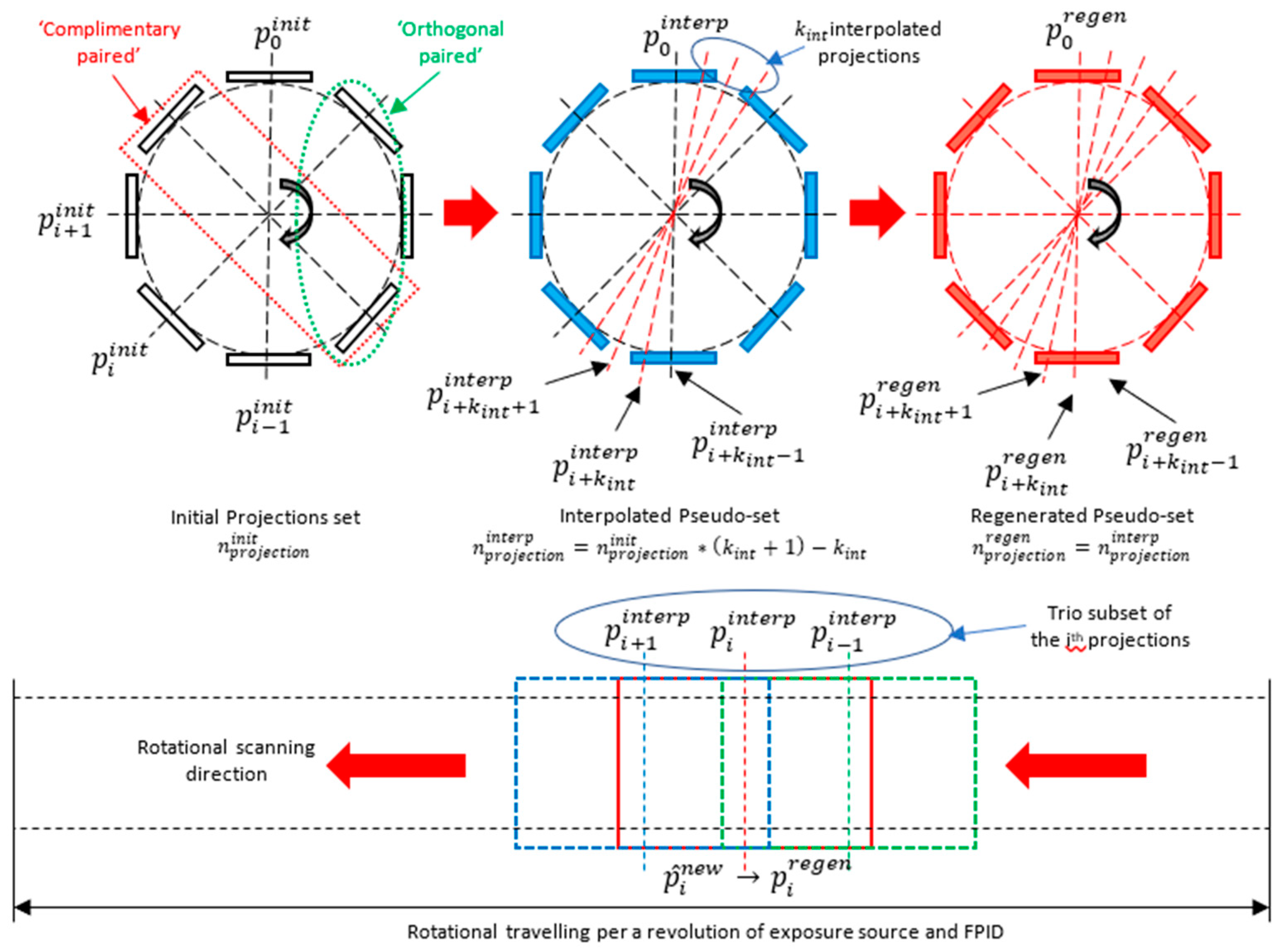
Firstly, the interpolation enrichment is implemented by Algorithm 1. The initial projection set is sparse viewed, so the proposal of input set enrichment is implemented by the interpolation as a denser pseudo-set of projections with the projection number to adapt the completeness of the basic computed tomography (CT) reconstruction fundamentals. Secondly, to enhance the projections set quality, our algorithm does not use the prior regularization as the others, but a loop of an “estimating–filtering–verifying” process for the regenerative interpolation (pseudo-) set of input projections is proposed to be applied with the same projection number . This is based on the pseudo-complete interpolated projection set before applying the final reconstruction. It is an enhancement process. The generative interpolation set of the initial projections set is implemented by updating the successive trio projection subset per each new projection. This is similar to a sliding window modulation. That regeneration is individualized per each normalized view of the full revolution, as shown in Figure 1. The prior projection, as , is used to estimate an in-flow overlapping of the successive one, as , in which the maximization is focused, which is termed the “Bhattacharyya distance” (), as shown in Equation (2). Based on the total similarity, proportional to , the updated projection for a new (pseudo-) set is estimated and pre-enhanced by the first two projections of a trio subset, respectively with the interpolated prior projection and the interpolated central projections, which is implemented via the discretized probability distribution.
wherein is called a “total similarity coefficient” (), which is defined by “Bhattacharyya coefficient” () of the pair of interpolated projections, of and , while is called the “estimated operator”, which is defined as shown in Equation (3).
The central projection, as a kernel of , is used to filter the result of , while the posterior projection, as , is used to verify the , the updated regenerative projection, as = , in which the minimization of is focused and termed as Kullback–Leibler’s divergence conditioning, as its distance () is shown in Equation (4). Then, the verification is implemented by the informative discrimination between the and the posterior one, , to update the regenerative projections as , if the informative discrimination is not exceeded (computational parameter). Otherwise, . The is the proper state of , which is modified by the -norm of the relevant to , as shown in Equation (5).
wherein and is called “verification operator”.
Let be the “absolute informative discrimination” of the verification at the ith projection, which is shown in Equation (5), as:
Let , where is called the “relative informative discrimination” between the estimated and the origin of the ith interpolated projection . Substituting in Equation (6), we have:
So, the updated projection is assigned to the regenerated projections set by “verification operator”, which is defined as shown in Equation (7):
| Algorithm 1: “Densification enrichment process” or Pseudo-Set Interpolation |
| Input: Initial projection set captured by FPID, as follows: Output: Interpolated pseudo-set for the reconstruction completeness availability, as follows: Begin Initialize necessary parameters. For k = 1 to k = maximum number of iterations: 1: , , and: . Find the common projection angle coincidences of two sets: and 2: Assign a kernel to remove the non-attenuated outer-cored region of interest (ROI). Implement the iteration loop by times. Then, assign the targeted pseudo-set with a denser viewed set, implanted with more interpolated projections in each interval of , between and . 3: Correct iteratively the implanted interpolated projections’ sinograms quality by structural similarity and mean squared errors with the given number of iterations. Assign the corrected ones as the final interpolated pseudo-set . End |
Our proposed enhancement process of the pseudo-set is shown in Algorithm 2.
| Algorithm 2: “Quality enhancement process” or Pseudo-Set Trio Subset Enhancement Operator |
| Input: Interpolated pseudo-set, as followed: Output: Regenerative pseudo-set for reconstruction, as follows: Begin 1: , and: 2: Apply the trio subset’s “estimating–filtering–verifying” processing loop per each projection in the interpolated pseudo-set iteratively.
End |
Finally, the output three-dimensional reconstruction is computed by our proposed variation of simultaneous iterative reconstruction technique (SIRT), which is called SA2IT (selective anatomy analytic iteration technique). The SIRT-based solution is chosen due to its advantage on the higher precision imaging quality reconstruction from the less accurate set of the appropriate noise-patterned projections, which is firstly introduced for medical computed tomography applications. However, its disadvantages are also mentioned in numerous studies, including (1) the expensive computational cost of the iteration, (2) the normalized blurring effect at the transition boundary of the less-intensity-discriminated levels, and (3) globalized intensity scale shifting, bandwidth truncating, and warping intensity distribution. Additionally, the effects of the background intensity levels affect the global contrast of an image, and the human-stimulated vision (as Weber’s Law) will be ignored in this study. The proposed SA2IT is conceptualized as a SIRT variation with constraints regarding the post-reconstruction average volumetric stabilization coefficients, which is recalled from any view of the prime input projections. This is constructed by the complimentary paired and the orthogonal paired projections. The proposed workflow is shown in Algorithm 3. As an iterative reconstruction technique, the generalization of Equation (8) for SA2IT is applied in this algorithm.
wherein:
where is the iteration number, is a noise reduction relaxation parameter, and are weighted coefficients for the back-projection and correction computation of the projection, successively, and is the correction computation based on the forward projection. The is the convergence condition recommended by Byrne et al. [29]. Additionally, the orthogonality featured convergence condition, , is proposed by our SA2IT, in which and are known as the orthogonality-featured bounded volume and the gradient descent SIRT (GD-SIRT) reconstructed volume. The corresponded correction computation is indicated in the term of the denser pseudo-set (), which is enriched, and enhanced by trio-subset principle as above.
| Algorithm 3: SA2IT algorithm |
| Input: Regenerative pseudo-set, as follows: Output: The SA2IT results Begin Initialize necessary parameters. For k = 1 to k = maximum number of iterations: 1: Apply the conventional SIRT algorithm to compute forward projection , correction computation (), back-projection, and the reconstructed volume , by Equations (8) and (9). 2: Apply the gradient descent to the reconstructed 3: Assign the corrected ones, adapted . End |
3. Experimental Setup
3.1. Phantom Reconstruction Experiments
As mentioned in dental literature and professional protocols, dental cone-beam computed tomography is used to give more clinical evidence for treatment planning and monitoring, which is anatomically relevant to hard tissues and various sinuses and air cavities of the maxillofacial region as well as dental structures. In ALADA’s radiation safety standard, the exposure dose is accurately managed to maintain the quality of diagnostic ability while strictly conforming to the patient’s radiation safety. Therefore, the experiments are designed as a sparse–viewed exposure of X-ray to lower the dosage per projection. This is different from the other algorithms; the proposed SA2IR enriches the input projection set with various sparsity, which is formulated with the densifying factorization or pseudo-up-sampling, to implant the possible slice into the sinogram of the original input. The specific number of input projections is set to minimum due to the trio-subset featured enhancement (a subset of three projections’ enhancement) and the orthogonality (periodic quadrant orthogonality per revolution) of the algorithm. When then SA2IR algorithm is applied, the pseudo-set is quantitatively enriched and qualitatively enhanced. Its reconstruction is based on SA2IT and was introduced in Part 4. In this work, the modified Shepp–Logan phantom, a variant of the numerical phantom for computed tomography simulation suggested by Shepp and Logan (1974) [30], was used to simulate the studied experiment results. For the clinical simulation, the realistic digital three-dimensional head phantom for C-Arm computed tomography supported by Aichert et al. (2013) [31] was used to simulate the clinical applicability of the algorithm in dental diagnostic imaging.
3.2. Comparison with the Other Reconstruction Algorithms
The reconstructed result of the proposed SA2IR algorithm is compared to the results of other algorithms, such as the Feldkamp–Davis–Kress (FDK) Algorithm [32], simultaneous iterative reconstruction technique (SIRT) [33], simultaneous algebraic reconstruction technique algorithm (SART) [34], order-subset SART (OS-SART) [35], total variation SART (TV-SART), adaptive steepest descent projection onto convex sets (ASD-POCS) [36], order-subset ASD-POCS (OS-ASD-POCS) [36], and conjugated gradient least square algorithm (CGLS) [37], and fast iterative shrinkage-thresholding algorithm (FISTA). Furthermore, the application of the trio-subset enhancement process to the sparse input of those is also implemented and studied.
4. Results and Discussions
4.1. Results of the SA2IR Algorithm’s Reconstruction Simulation
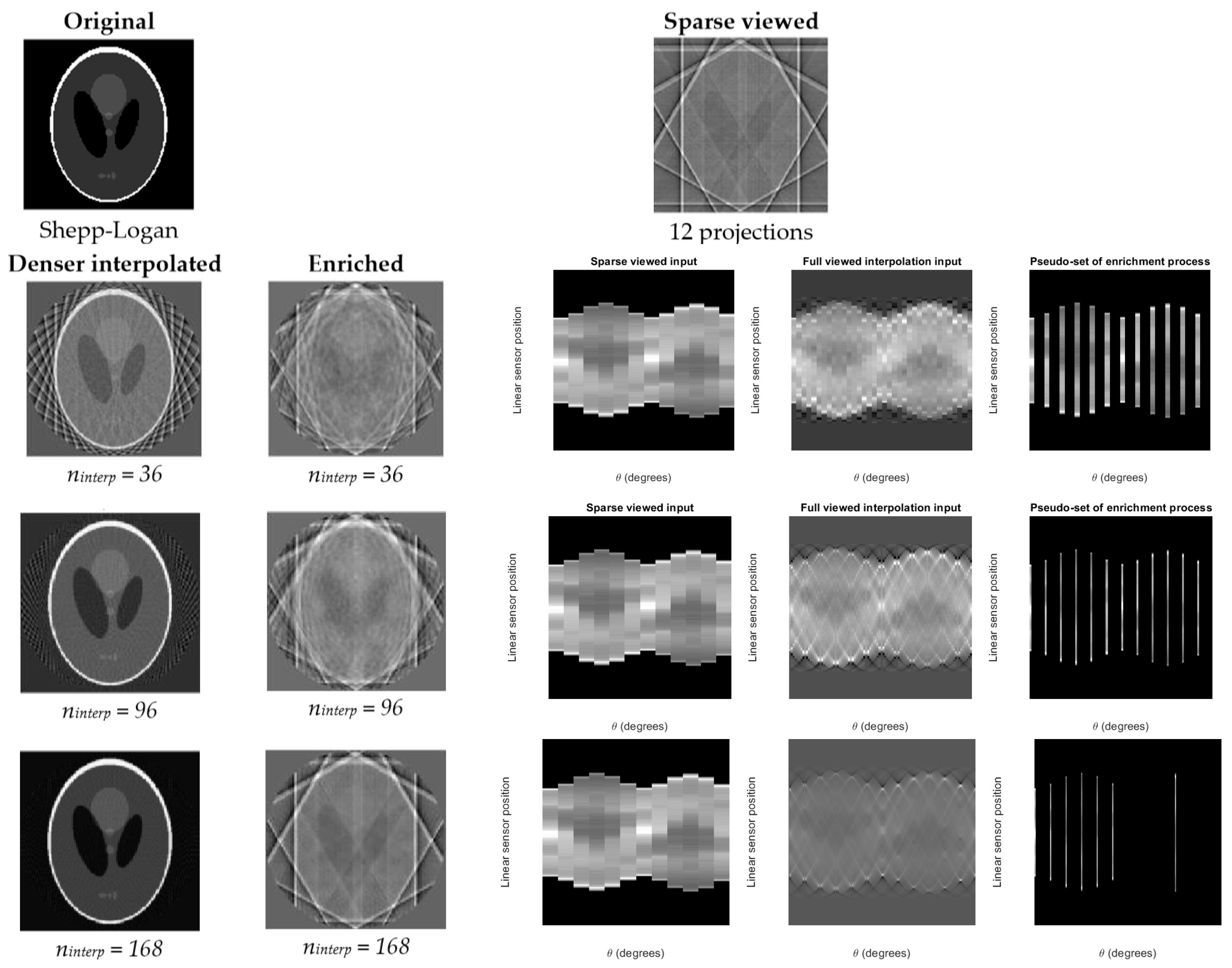
The simulated results of the proposed SA2IR are demonstrated into three parts: (a) the pseudo-set enrichment process, (b) the trio-subset enhancement process, and (c) the SA2IT reconstruction, respectively. The results are conducted on the modified Shepp–Logan phantom and the realistic patient’s head data. The simulations are implemented in the MATLAB environment (MATLAB 2017b, The MathWorks Inc., Natick, Massachusetts, USA) and tomographic iterative GPU-based reconstruction framework [38]. The simulations are based on the configuration of DCT100-0x0 CBCT (shown in Table 1) and implemented with the compilation support of the Nvidia CUDA toolkit 10.1, accelerated by Nvidia GTX 1650 GPU. Corresponding to the experimental setup, the specific number of input projections is simulated at the minimum of 12 projections (conducted by the ksparse = 6), which was demonstrated with the odd and even quadrant-bases number. The simulation results are conducted with ksampling values of 3, 8, and 14, which successively corresponded to the number of interpolated projections of 36, 96, and 168. The relevant sinograms of the enrichment process for the cases, including those sparse projections, denser projections, and enriched projections sets, are shown in Figure 2. Obviously, the lesser number of projection input is, the lower the reconstruction quality. Therefore, our proposed algorithm inserts the common between a sparse input to the denser expectation, with the given ksampling values of 3, 8, and 14, respectively as the number of projections in the enriched pseudo-sets. That made no changes in the histograms. However, it made a bounding enhancement. The generative noise is patterned as two parts, as external and internal patterned effects. The external patterned effect is shown as the bright streaked bounded frames and the aliased interfere, which is proportional to the times of overlapping, in terms of the common interaction of those, while the internal patterned effect is shown as a cumulative “edge-blurring”. It causes an effect, which is similar to contrast diffusion from the internal patterned out to the external patterned part, in the meaning of gradient, while preserving the histogram. That is partly also discussed by Perona and Malik regarding the Perona–Malik diffusion, which is known as a nonlinear anisotropic diffusion and is equivalent to Gaussian blurring in the case of constant diffusion coefficient, as a conventional heat equation [39]. In the case of SA2IR enrichment, the noise pattern is disturbed by the spacing of the interpolation. The densification of those depends on the overlapping of the common projections of the initial and the pseudo-set, which would be normally distributed (ninterp = 96 and 144) or partly compressed (ninterp = 168). Due to the symmetricity of the phantom, the orthogonality repetition base on equilateral segments is studied, which shows the behavior of the pseudo-set’s cumulative noise pattern. That orthogonality of the post-enrichment processing interpolated pseudo-set is also shown via eight equilateral segments of one scanning revolution (45 degrees per each segment), which are named successively as Ω1, Ω2, …, Ω7 and Ω8. The pattern and deterioration of the orthogonality per each segment are detected. The noise distribution changes per one scanning revolution; especially at the transition points at 0 degrees and 360 degrees, the flattened effect is observed. Otherwise, the shifting effects and blurring are differentiated per orthogonality pattern and the deterioration of each segment.
The parameters of trio-subset enhancement processing, such as the estimation operator (), filtering operator (), verification operator (), and their representation, are called ‘total trio-subset enhancement operator’ (), which is shown quantitively in Table 2. The contribution of the operators on the total enhancement operator () is calculated, which corresponded to the overlapped indices of each projection with its prior and posterior projections. The results show the efficiency of the bilateral approximation to construct a new pseudo-set of the same interpolated projections. The results and the relationship between the estimation and verification processes of three cases A, B, and C, with the specific common views or projections in each segment Ωi are shown in Table 2, between , and . Those specific common views are categorized as the first, middle, and last projections groups; these describe the behavior of each process per each segment Ωi and per different cases, which are set with 96, 144, and 168 projections to generate a new pseudo-set prior to the reconstruction.
Additionally, the results also show that the overlapping coefficient, , is meaningful in relation to the values regarding the number of projections and the operators in the trio sub-set enhancement. This coefficient is defined in Equation (9).
wherein is the distance between the detector and subject, is the width of the detector, and is the number of interpolated projections of the pseudo-set.
Three cases A, B, and C, defined as sparse 12 projections’ input, and the ninterp = 96, 144, and 168. The A, B, and C result sets are quoted at the first, middle, and last projections of each segment Ωi (i = [1,8], I ∈ ℕ). The Ωi is defined in degrees of (0,45), (45,90), (90,135), … (270,315), (315,360). The notation explanation of the common first, middle, and last projections represented for each segment of those cases is shown in Table 3.
4.2. Comparison to the Other Reconstruction Algorithms
The reconstructed results are implemented on the sparse 12-projection set, the result of the proposed SA2IR is compared to different algorithms, as mentioned above, included FDK, SIRT, SART, OS-SART, TV-SART, ASD-POCS, OS-ASD-POCS, β-ASD-POCS, CGLS, and FISTA. Obviously, the sparse set is unable to be implemented with FDK; the other results are shown in Figure 3. The result of our proposed algorithm (Figure 3(k1)) for the sparse case shows the transition quality between the results of SIRT (Figure 3(b1)) and SART (Figure 3(c1)). The edge preservation of the proposed algorithm is better than that of the conventional SIRT and nearly the same as that of SART. The external generative noise is a little bit thinner than the result of SIRT, while the internal generative noise is likely homogenous and better than the result of SART. Furthermore, the proposed algorithm shows that the edge preservation and global homogeneity are significantly better than the other results of OS-SART (intensity reducing), TV-SART (informative loss of edge and intensity), ASD-POCS (structural similarity reducing), OS-ASD-POCS (blurring), β-ASD-POCS (edge and intensity deterioration), CGLS (edge blurring), and FISTA (total image quality reducing) (in Figure 3, from (d1) to (j1)). Consequently, in the case of sparse projection input, the proposed algorithm reduced the generative noise significantly, compared to the other algorithms, as mentioned above, while preserving the edge and intensity; thus, had diagnostic ability.
The reconstructed results are implemented on the denser projection set of 48, as shown in Figure 3 (from (a2) to (l2). The result of the SA2IR algorithm is compared to different algorithms, as mentioned above, included SIRT, SART, OS-SART, TV-SART, ASD-POCS, OS-ASD-POCS, β-ASD-POCS, CGLS, and FISTA. In this section, we implemented both results of the proposed algorithm, as the origin and the modified ones, successively shown in Figure 3(k2,l2). The results are shown to be the same as what was discussed in the case of the sparse projection input.
Due to the shape-ness characteristics, the noise distributions are shown patterned per segments. The boundary ripple causes the edge detail loss, and the shifting causes the intensity loss. The image quality metrics of the reconstructed results are qualitatively evaluated in Table 4. The qualitative metrics of image quality are proposed to be measured in root mean square error (RMSE), structural similarity (SSIM), peak signal-to-noise ratio (PSNR), and signal-to-noise (SNR), and the entropy of the results are shown in Figure 3. According to Table 4, the quantitative metric benefits of SA2IR are indicated as asterisked. Those metrics are divided into two main groups, included (1) the Referral metrics group, included RMSE, SSIM, PSNR, and SNR, which is referred to the original phantom, and (2) the Individual metrics group, as the entropy measurement. Corresponding to the results in Figure 3 and Table 4, the proposed SA2IR algorithm is proved to reduce the generative noise, both external and internal of the edges, or inner or outer of the edge, compared to the other algorithms.
For the patient head data clinical simulation, the reconstructed results are implemented and demonstrated into the different section of maxillofacial and mandibular structures (shown in Figure 4). The reconstruction was done with the initial sparse set of 68 projections. The enrichment ratio was chosen as ksampling = 8 for doubling scan angular rotation. Those results are addressed as the upper jaw region (basal palatine bone), lower arch, mid-facial region, and temporomandibular joint region, respectively to the 68th, 52nd, 108th, and 112nd slices of the used patient head data (shown in Figure 5). The boxing volumetric size of the head data reconstruction is 360 × 360 × 360 (in mm). According to the simulation results of the phantom in Table 4, the qualitative image quality metric evaluation of those is shown in Table 5. Regarding the meaning of image quality indexes and computational time “trade-off”, the significant benefit of using the proposed algorithm compared to the other common contemporary algorithms for sparse projection reconstruction was observed. According to the results in Figure 3, the reconstructed results of the clinical simulation is to compare SA2IR to SIRT, SART, OS-SART, ASD-POCS, OS-ASD-POCS, and CGLS algorithms. The remainder were omitted, because of their disadvantages when compared to the SA2IR. To clarify the trade-off beneficiary of SA2IR to the others, the differentiation beneficiary is shown in Table 5.
According to Table 5, the results of the proposed algorithm are significantly beneficiary in balancing between the ALADA adaptation and computation time (in seconds) in comparison to the other referred algorithms. To evaluate the “clinical diagnostic-ability”, the mean square error (MSE), structural similarity (SSIM), entropy (E), and the signal-to-noise ratios (PSNR and SNR) are used. In the complicative structures of the mid-facial and temporomandibular joint regions, the results of SA2IR are shown to be better than those of SART and ASD-POCS. The results are shown to have no meaningful diagnostic-able visual differences compared to OS-SART and OS-ASD-POCS. Except for the computation time of the SIRT and CGLS algorithms, SA2IR took less time to implement than the others. The computation time that the SA2IR algorithm took was 4.8, 5.0 and 5.3 s, which are significantly less when compared to SART (30.2, 30.2 and 35.1 s) and ASD-POCS (32.0, 35.9 and 37.1 s), while arithmetically less than that of OS-SART (5.4, 5.3 and 5.8 s) and OS-ASD-POCS (5.3, 5.3 and 5.6 s). However, the image quality of SIRT and CLGS is lower and has more blurring than the other algorithms, as shown in Figure 5. The SA2IR result has similar effects to the ordered-subset regularizations of both ASD-POCS and SART in generative noise reduction, contrast equalization, and cost-effective computation. Furthermore, the generative noise reduction in SA2IR is less than all the other algorithms shown in Figure 5. This is due to the “chirp soft ablation” effect of the trio subsets enhancement of SA2IR.
The proposed algorithm shows good agreement with the trade-off problem when using sparse projections to design low-dosed CBCT reconstructions. The results are promising when compared to other algorithms due to the balanced image quality, diagnostic potential, along with more cost-effective computation, and lowered exposure. The generative noise reduction effect is significantly reduced due to the initial projects set densification (enrichment) and trio subset enhancement. The structural features and contrast are maintained as able to be diagnostic. The computation time has been reduced significantly in comparison to the other algorithms such as SART, OS-SART, ASD-POCS, and OS-ASD-POCS.
5. Conclusions
In this paper, the SA2IR is proposed as a specific iterative method for dental CBCT reconstruction problems. This algorithm is made up of two parts: the pre-reconstruction processing and the 3D reconstruction of a CBCT projection set. The pre-reconstruction process is composed of the pseudo-set enrichment and the trio-subset enhancement processes. Experimental simulation was implemented with (1) a minimum projection set of 12 projections and (2) the sparse cases of 48 projections, on a phantom. Clinical simulation was implemented with the sparse projections set of 68 projections, with respect to the diagnostic anatomy differentiation of four regions. These regions are the upper jaw arch, lower jaw arch, mid-facial, and temporomandibular. The results have shown that when compared to previous conventional algorithms (SIRT, SART, OS-SART, ASD-POCS, OS-ASD-POCS, and CGLS), the SA2IR method produces comparable diagnostic ability image quality compared to the other conventional methods. SA2IR reduces generative noise, can preserve structural features, and has enhanced global contrast when compared to SART, OS-SART, ASD-POCS, and OS-ASD-POCS. The SA2IR’s computation time is significantly better than all of the other methods, especially when compared to SART and ASD-POCS. The clinical simulation has shown the compatibility of the algorithm with many applied dental image diagnostics, especially for dental implantology and maxillofacial surgery.
The proposed algorithm is shown to be highly applicable in the sparse projection and low-dose CBCT reconstruction, adapting the ALADA concept, as “radiation safer and imaging diagnostic-ability optimization”. That is more humane for the patients and clinicians, regarding both heath and responsibility. This approach is also available to be applied in other medical CBCT reconstruction applications. This selective anatomical analytic iteration reconstruction (SA2IR) algorithm uses a combination of the regularization approach and statistical approach, and utilizes the robustness of GPU-based computation. To improve upon this study, further research will be conducted on human head and body anatomy structures and properties. That study will help to enhance the SA2IR’s trio subset enhancement process. The bio-physical relationship will aid in modeling between exposure–direction and various other anatomical structures. The outcome of this experiment is expected to reduce generative noise as well as computational uncertainties, and enhance the imaging of the soft tissue structure.
Author Contributions
Y.-C.D. and L.D.-N. developed the methodology. Y.-C.D. conceived, supervised, and coordinated the investigations as well as checked the manuscript’s logical structure. L.D.-N. performed the simulation as well as analyzed the experimental data.
Funding
The authors would like to thank the Ministry of Education, Taiwan, for financially supporting this research in the Allied Advanced Intelligent Biomedical Research Center (A2IBRC) under the Higher Education Sprout Project.
Conflicts of Interest
The authors declare no conflict of interest.
Abbreviations
The following abbreviations are used in this manuscript:
| ALADA | As Low As Diagnostically Acceptable |
| ALARA | As Low As Reasonably Achievable |
| (OS)-ASD-POCS | (Order-Subset) Adaptive Steepest Descent Projection On Convex Sets |
| CAD/CAM | Computer-Aided Design/ Computer -Aided Manufacturing |
| CBCT | Cone-Beam Computed Tomography |
| CGLS | Conjugated Gradient Least Square |
| CT | Computed Tomography |
| DICOM | Digital Imaging and Communication in Medicine |
| FISTA | Fast Iterative Shrinkage-Thresholding Algorithm |
| FPID | Flat Panel Imaging Detector |
| FDK | Feldkamp - Davis - Kress |
| GPU | Graphical Processing Unit |
| NCRP | National Council on Radiation Protection (United States) |
| RMSE | Root Mean Square Error |
| SA2IR | Selective Anatomy Analytic Iteration Reconstruction |
| SA2IT | Selective Anatomy Analytic Iteration Technique |
| (OS)-SART | (Order-Subset) Simultaneous Algebraic Reconstruction Technique |
| SIRT | Simultaneous Iterative Reconstruction Technique |
| SNR | Signal-To-Noise Ratio |
| PSNR | Peak Signal-To-Noise Ratio |
| SSIM | Structural Similarity |
| TSC | Total Similarity Coefficient |
References
- Fokas, G.; Vaughn, V.N.; Scarfe, W.C.; Bornstein, M.M. Acccuracy of linear measurement on CBCT images related to presurgical implant treatment: A systematic review. Clin. Oral Implant. Res 2018, 29, 393–415. [Google Scholar] [CrossRef] [PubMed]
- Bornstein, M.M.; Jorner, K.; Jacobs, R. Use of cone beam computed tomography in implant dentistry: Current concepts, indications, and limitations for clinical practice and research. Periodontology 2017, 73, 51–72. [Google Scholar] [CrossRef] [PubMed]
- Kim, I.H.; Singer, S.R.; Mupparapu, M. Review of cone beam computed tomography guidelines in North America. Quintessence Int. 2019, 50, 136–145. [Google Scholar]
- Hayashi, T.; Arai, Y.; Chikui, T.; Hayashi-Sakai, S.; Honda, K.; Indo, H.; Kawai, T.; Kobayashi, K.; Murakami, S.; Nagasawa, M.; et al. Committee on Clinical Practice Guidelines Japanese Society for, Oral Maxillofacial, Radiology. Clinical guidelines for dental cone-beam computed tomography. Oral Radiol. 2018, 34, 89–104. [Google Scholar] [CrossRef]
- Alghazzawi, T.F. Advancements in CAD/CAM technology: Options for practical implementation. J. Prosthodont. Res. 2016, 60, 72–84. [Google Scholar] [CrossRef]
- Dao-Ngoc, L. The review of RP (Rapid Prototyping application in maxillofacial surgeries in Vietnam from 2010 to 2016: In the manufacturing engineer’s view. Cập nhật nha khoa–Tài liệu tham khảo và đào tạo liên tục 2017, 22, 121–142. [Google Scholar]
- Qin, Z.; Zhang, X.; Li, Y.; Wang, P.; Li, J. One-stage treatment for maxillofacial asymmetry with orthognathic and contouring surgery using virtual surgical planning and 3D-printed surgical templates. J. Plast. Reconstr. Aesthet. Surg. 2019, 72, 97–106. [Google Scholar] [CrossRef]
- Bushberg, J.T. Eleventh annual Warren K. Sinclair keynote address-science, radiation protection and NCRP: Building on the past, looking to the future. Health Phys. 2015, 108, 115–123. [Google Scholar] [CrossRef]
- White, S.C.; Scarfe, W.C.; Schulze, R.K.W.; Lurie, A.G.; Douglass, J.M.; Farman, A.G.; Law, C.S.; Levin, M.D.; Sauer, R.A.; Valachovic, R.W.; et al. The Image Gently in Dentistry campaign: Promotion of responsible use of maxillofacial radiology in dentistry for children. Oral Surg. Oral Med. Oral Pathol. Oral Radiol. 2014, 118, 257–261. [Google Scholar] [CrossRef]
- Fernandes, K.; Levin, T.L.; Miller, T.; Schoenfeld, A.H.; Amis, E.S., Jr. Evaluating an Image Gently and Image Wisely Campaign in a Multihospital Health Care System. J. Am. Coll. Radiol. 2016, 13, 1010–1017. [Google Scholar] [CrossRef]
- Jaju, P.P.; Jaju, S.P. Cone-beam computed tomography: Time to move from ALARA to ALADA. Imaging Sci. Dent. 2015, 45, 263–265. [Google Scholar] [CrossRef]
- Matenine, D.; Goussard, Y.; Despres, P. GPU-accelerated regularized iterative reconstruction for few-view cone beam CT. Med. Phys. 2015, 42, 1505–1517. [Google Scholar] [CrossRef]
- Zhang, H.; Wang, J.; Zeng, D.; Tao, X.; Ma, J. Regularization strategies in statistical image reconstruction of low-dose X-ray CT: A review. Med. Phys. 2018, 45, e886–e907. [Google Scholar] [CrossRef]
- Jacobs, R.; Vranckx, M.; Vanderstuyft, T.; Quirynen, M.; Salmon, B. CBCT vs. other imaging modalities to assess peri-implant bone and diagnose complications: A systematic review. Eur. J. Oral Implant. 2018, 11, 77–92. [Google Scholar]
- Katsumata, A.; Hirukawa, A.; Okumura, S.; Naitoh, M.; Fujishita, M.; Ariji, E.; Langlais, R.P. Effects of image artifacts on gray-value density in limited-volume cone-beam computerized tomography. Oral Surg. Oral Med. Oral Pathol. Oral Radiol. Endodontol. 2007, 104, 829–836. [Google Scholar] [CrossRef]
- Stefanelli, L.V.; DeGroot, B.S.; Lipton, D.I.; Mandelaris, G.A. Accuracy of Dynamic Dental Implant Navigation System in a Private Practice. Int. J. Oral Maxillofac. Implant. 2019, 34, 205–2013. [Google Scholar] [CrossRef]
- Harris, B.T.; Montero, D.; Grant, G.T.; Morton, D.; Llop, D.R.; Lin, W.S. Creation of a 3D dimensional virtual dental patient for computer-guided surgery and CAD-CAM interim complete removable and fixed dental prostheses: A clinical report. J. Prosthet. Dent. 2017, 117, 197–204. [Google Scholar] [CrossRef]
- Patel, S.; Brown, J.; Pimentel, T.; Kelly, R.D.; Abella, F.; Durack, C. Cone beam computed tomography in Endodontics—A review of the literature. Int. Endod. J. 2019, 52, 1138–1152. [Google Scholar] [CrossRef]
- Tchorz, J.P. 3D Endo: Three-dimensional endodontic treatment planning. Int. J. Comput. Dent. 2017, 20, 87–92. [Google Scholar]
- Woelber, J.P.; Fleiner, J.; Rau, J.; Ratka-Kruger, P.; Hannig, C. Accuracy and Usefulness of CBCT in Periodontology: A Systematic Review of the Literature. Int. J. Periodontics Restor. Dent. 2018, 38, 289–297. [Google Scholar] [CrossRef]
- Pozzi, A.; Arcuri, L.; Moy, P.K. The smiling scan technique: Facially driven guided surgery and prosthetics. J. Prosthodont. Res. 2018, 62, 514–517. [Google Scholar] [CrossRef] [PubMed]
- McGuigan, M.B.; Duncan, H.F.; Horner, K. An analysis of effective dose optimization and its impact on image quality and diagnostic efficacy relating to dental cone beam computed tomography (CBCT). Swiss Dent. J. 2018, 128, 297–316. [Google Scholar]
- Karimi, D.; Ward, R.K. Sinogram denoising via simultaneous sparse representation in learned dictionaries. Phys. Med. Biol. 2016, 61, 3536–3553. [Google Scholar] [CrossRef]
- Zhu, Z.G.; Wahid, K.; Babyn, P.; Cooper, D.; Pratt, I.; Carter, Y. Improved Compressed Sensing Based Algorithm for Sparse—View CT Image Reconstruction. Comput. Math. Methods Med. 2013, 2013, 185750. [Google Scholar] [CrossRef]
- Zhang, H.M.; Li, L.; Wang, L.Y.; Sun, Y.M.; Yan, B.; Cai, A.L.; Hu, G.E. Computed Tomography Sinogram Inpainting With Compound Prior Modelling Both Sinogram and Image Sparsity. IEEE Trans. Nucl. Sci. 2016, 63, 2567–2576. [Google Scholar] [CrossRef]
- Zhang, C.; Zhang, T.; Zheng, J.; Li, M.; Lu, Y.; You, J.; Guan, Y. A Model of Regularization Parameter Determination in Low-Dose X-Ray CT Reconstruction Based on Dictionary Learning. Comput. Math. Methods Med. 2015, 2015, 831790. [Google Scholar] [CrossRef]
- Du, D.; Pan, Z.; Zhang, P.; Li, Y.; Ku, W. Compressive sensing image recovery using dictionary learning and shape-adaptive DCT thresholding. Magn. Reson. Imaging 2019, 55, 60–71. [Google Scholar] [CrossRef]
- Kim, G.; Park, S.; Je, U.; Cho, H.; Park, C.; Kim, K.; Lim, H.; Lee, D.; Lee, H.; Park, Y.; et al. A New Voxelization Strategy in Compressed-Sensing (CS)-Based Iterative CT Reconstruction for Reducing Computational Cost: Simulation and Experimental Studies. J. Med. Biol. Eng. 2018, 38, 129–137. [Google Scholar] [CrossRef]
- Byrne, C. A unified treatment of some iterative algorithms in signal processing and image reconstruction. Inverse Probl. 2003, 20, 103–120. [Google Scholar] [CrossRef]
- Shepp, L.A.; Logan, B.F. The Fourier reconstruction of a head section. IEEE Trans. Nucl. Sci. 1974, 21, 21–43. [Google Scholar] [CrossRef]
- Aichert, A.; Manhart, M.T.; Navalpakkam, B.K.; Grimm, R.; Hutter, J.; Maier, A.; Hornegger, J.; Doerfler, A. A realistic digital phantom for perfusion C-arm CT based on MRI data. In Proceedings of the 2013 IEEE Nuclear Science Symposium and Medical Imaging Conference (2013 NSS/MIC), Seoul, Korea, 27 October–2 November 2013. [Google Scholar]
- Feldkamp, L.A.; Davis, L.C.; Kress, J.W. Practical Cone-Beam Algorithm. J. Opt. Soc. Am. A 1984, 1, 612–619. [Google Scholar] [CrossRef]
- Kak, A.C.; Slaney, M. Principles of Computerized Tomographic Imaging, Classics in Applied Mathematics; Society for Industrial and Applied Mathematics: Philadelphia, PA, USA, 2001. [Google Scholar] [CrossRef]
- Andersen, A.H.; Kak, A.C. Simultaneous Algebraic Reconstruction Technique (SART)—A Superior Implementation of the ART Algorithm. Ultrason. Imaging 1984, 6, 81–94. [Google Scholar] [CrossRef]
- Censor, Y.; Elfving, T. Block-iterative algorithms with diagonally scaled oblique projections for the linear feasibility problem. SIAM J. Matrix Anal. Appl. 2002, 24, 40–58. [Google Scholar] [CrossRef]
- Sidky, E.Y.; Pan, X. Image reconstruction in circular cone-beam computed tomography by constrained, total-variation minimization. Phys. Med. Biol. 2008, 53, 47–77. [Google Scholar] [CrossRef]
- Björck, Å. Numerical Methods for Least Squares Problems; Society for Industrial and Applied Mathematics: Philadelphia, PA, USA, 1996. [Google Scholar] [CrossRef]
- Biguri, A.; Dosanjh, M.; Hancock, S.; Soleimani, M. TIGRE: A MATLAB-GPU toolbox for CBCT image reconstruction. Biomed. Phys. Eng. Express 2016, 2, 055010. [Google Scholar] [CrossRef]
- Perona, P.; Malik, J. Scale-space and edge detection using anisotropic diffusion. IEEE Trans. Pattern Anal. Mach. Intell. 1990, 16, 629–639. [Google Scholar] [CrossRef] [Green Version]
Figure 1.
The illustrations of the projection set and the trio subset in selective anatomy analytic iteration reconstruction (SA2IR).
Figure 1.
The illustrations of the projection set and the trio subset in selective anatomy analytic iteration reconstruction (SA2IR).

Figure 2.
The reconstruction and sinograms illustration of the enrichment process of a sparse 12 projections (original, the first row), at the denser interpolated set of 36 (upper-left) (the second row), 96 (upper-right), and 168 projections (the third row).
Figure 2.
The reconstruction and sinograms illustration of the enrichment process of a sparse 12 projections (original, the first row), at the denser interpolated set of 36 (upper-left) (the second row), 96 (upper-right), and 168 projections (the third row).

Figure 3.
The Shepp–Logan phantom reconstructed results, based on sparse 12-projection input (from (a1) to (k1)) and sparse 48-projection input (from (a2)–(l2)), such as: (a1,a2)–Origin phantom, (b1,b2)–SIRT (simultaneous iterative reconstruction technique), (c1,c2)–SART (simultaneous algebraic reconstruction technique algorithm), (d1,d2)–OS-SART (order-subset SART), (e1,e2)–TV-SART (total variation SART), (f1,f2)–ASD-POCS (adaptive steepest descent projection onto convex sets), (g1,g2)–OS-ASD-POCS (order-subset ASD-POCS), (h1,h2)–β-ASD-POCS, (i1,i2)–CGLS (conjugated gradient least square algorithm), (j1,j2)–FISTA (fast iterative shrinkage-thresholding algorithm) and (k1,k2)–SA2IR.
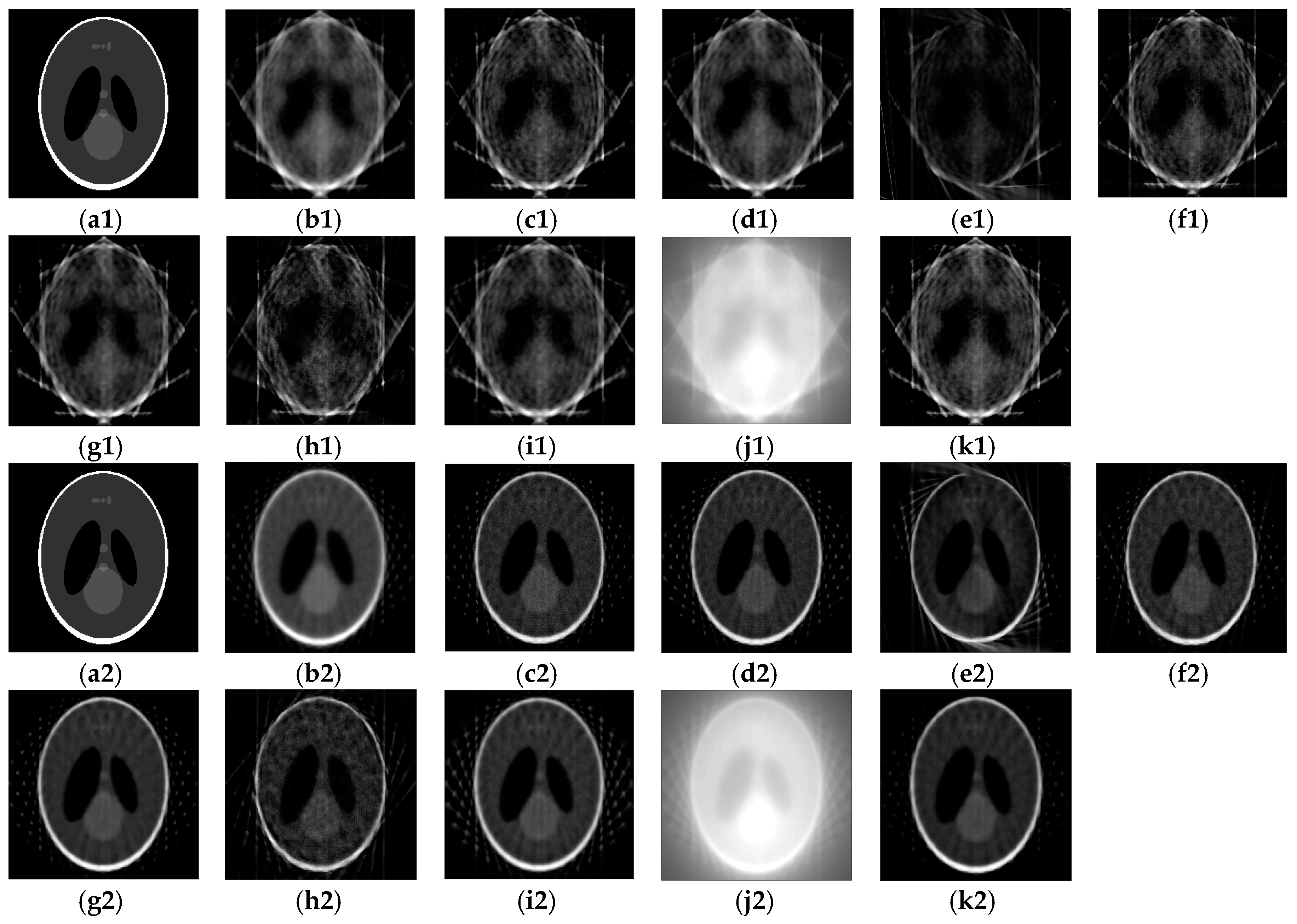
Figure 4.
The patient head data referred to dental anatomical regions (from left to right), such as: (a)–Upper jaw region (at slice #68), (b)–Lower arch (at slice #52), (c)–Mid-facial region (at slice #108), (d)–Temporomandibular joint region (at slice #112).
Figure 4.
The patient head data referred to dental anatomical regions (from left to right), such as: (a)–Upper jaw region (at slice #68), (b)–Lower arch (at slice #52), (c)–Mid-facial region (at slice #108), (d)–Temporomandibular joint region (at slice #112).

Figure 5.
The reconstructed results of others algorithms compared to SA2IR, with respect to the different anatomical regions, as: (a)–Upper jaw region (the first row), (b)–Lower arch (the second row), (c)–Mid-facial region (the third row), and (d)–Temporomandibular region (the fourth row).
Figure 5.
The reconstructed results of others algorithms compared to SA2IR, with respect to the different anatomical regions, as: (a)–Upper jaw region (the first row), (b)–Lower arch (the second row), (c)–Mid-facial region (the third row), and (d)–Temporomandibular region (the fourth row).


Table 1.
DCT100-0X0 cone-beam computed tomography (CBCT) technical configuration. FPID: flat-panel imaging detector.
Table 1.
DCT100-0X0 cone-beam computed tomography (CBCT) technical configuration. FPID: flat-panel imaging detector.
| Technical Parameters | Information | - | ||
|---|---|---|---|---|
| Notation | Unit | Value | ||
| Source-to-Detector Distance | SDD | cm | 72 | Term of “Patient” position means “Rotation Axis” position |
| Source-to-Patient Distance | SPD | cm | 50 | |
| Patient-to-Detector Distance | PDD | cm | 22 | |
| X-ray beam exposure size | WE × HE | cm × cm | 12.8 × 12.8 | Width × Height |
| Cone-beam opening of FPID | βx βz | (o) | 9.15° 9.15° | Respected to xx and yy axis |
| Detector’s size (Width × Length) | W × L | cm × cm | 13 × 13 | Amorphous Silicon Receptor |
| Voxel size | Vx | mm | 0.125 and 0.200 | - |
| Rotation degree | Α | (o) | 180° or 360° | Projection arch per scan |
| Field-of-View (Diameter × Height) | FOV (D × H) | cm × cm | 9 × 9 and 15 × 9 | - |
| Projection rotation angular step | αpst | (o/step) | 0.6 | - |
| Number of projections | Np | projections | 300 or 600 | np = α/pp |
Table 2.
The trio-subset enhancement operators of the simulated results.
| Simulated Results Based on the Modified Shepp–Logan Phantom | ||||||
|---|---|---|---|---|---|---|
| Processes | Estimation Process | Verification Process | ||||
| Studied Segments | - | |||||
| Ω1 | A 1,6,12 | 0.1634 | 0.8366 | 2.4442 | 2.4442 ± 2.0901 × 10⁻¹⁴ | 0.3215 |
| 0.0050 | 0.9950 | 2.4575 | 2.4575 ± 1.3341 × 10⁻¹⁴ | |||
| 0.0063 | 0.9937 | 2.4577 | 2.4577 ± 1.4675 × 10⁻¹⁴ | |||
| B 1,9,18 | 0.1283 | 0.8717 | 2.4576 | 2.4576 ± 2.2235 × 10⁻¹⁴ | 0.2139 | |
| 0.0052 | 0.9948 | 2.4575 | 2.4575 ± 4.4470 × 10⁻¹⁶ | |||
| 0.0046 | 0.9954 | 2.4575 | 2.4575 ± 2.1790 × 10⁻¹⁴ | |||
| C 1,11,21 | 0.1008 | 0.8992 | 2.4575 | 2.4576 ± 1.2451 × 10⁻¹⁴ | 0.1833 | |
| 0.0028 | 0.9972 | 2.4575 | 2.4575 ± 8.4492 × 10⁻¹⁵ | |||
| 0.0023 | 0.9977 | 2.4574 | 2.4575 ± 6.6704 × 10⁻¹⁵ | |||
| Ω2 | A 12,18,24 | 0.0063 | 0.9937 | 2.4577 | 2.4577 ± 1.4675 × 10⁻¹⁴ | 0.3215 |
| 0.0041 | 0.9959 | 2.4577 | 2.4577 ± 2.3569 × 10⁻¹⁴ | |||
| 0.0019 | 0.9981 | 2.4577 | 2.4577 ± 2.0011 × 10⁻¹⁴ | |||
| B 18,27,36 | 0.0046 | 0.9954 | 2.4575 | 2.4575 ± 2.1790 × 10⁻¹⁴ | 0.2139 | |
| 0.9324 | 0.9991 | 2.4575 | 2.4575 ± 7.5598 × 10⁻¹⁵ | |||
| 0.1033 | 0.9999 | 2.4575 | 2.4575 ± 8.4492 × 10⁻¹⁵ | |||
| C 21,32,42 | 0.0023 | 0.9977 | 2.4575 | 2.4575 ± 6.6704 × 10⁻¹⁵ | 0.1833 | |
| 0.0041 | 0.9959 | 2.4575 | 2.4575 ± 1.4230 × 10⁻¹⁴ | |||
| 0.3650 | 1.0000 | 2.4575 | 2.4575 ± 1.5120 × 10⁻¹⁴ | |||
| Ω3 | A 24,30,36 | 0.0019 | 0.9981 | 2.4577 | 2.4577 ± 2.0011 × 10⁻¹⁴ | 0.3215 |
| 0.3053 | 0.9997 | 2.4576 | 2.4576 ± 2.2401 × 10⁻¹⁴ | |||
| 0.9441 | 0.9999 | 2.4576 | 2.4576 ± 1.9122 × 10⁻¹⁴ | |||
| B 36,45,54 | 0.1033 | 0.9999 | 2.4575 | 2.4575 ± 8.4492 × 10⁻¹⁵ | 0.2139 | |
| 0.0016 | 0.9984 | 2.4575 | 2.4575 ± 5.7810 × 10⁻¹⁵ | |||
| 0.0056 | 0.9944 | 2.4575 | 2.4575 ± 1.6009 × 10⁻¹⁴ | |||
| C 42,53,63 | 0.3650 | 1.0000 | 2.4575 | 2.4575 ± 1.5120 × 10⁻¹⁴ | 0.1833 | |
| 0.1337 | 0.9999 | 2.4575 | 2.4575 ± 1.2451 × 10⁻¹⁴ | |||
| 0.0125 | 0.9875 | 2.4575 | 2.4575 ± 2.0901 × 10⁻¹⁴ | |||
| Ω4 | A 36,42,48 | 0.9441 | 0.9999 | 2.4576 | 2.4576 ± 1.9122 × 10⁻¹⁴ | 0.3215 |
| 0.0015 | 0.9985 | 2.4576 | 2.4576 ± 1.2451 × 10⁻¹⁴ | |||
| 0.0036 | 0.9964 | 2.4576 | 2.4576 ± 2.3124 × 10⁻¹⁴ | |||
| B 54,63,72 | 0.0056 | 0.9944 | 2.4575 | 2.4575 ± 1.6009 × 10⁻¹⁴ | 0.2139 | |
| 0.0102 | 0.9898 | 2.4575 | 2.4575 ± 1.9122 × 10⁻¹⁴ | |||
| 0.0060 | 0.9940 | 2.4575 | 2.4575 ± 1.0228 × 10⁻¹⁴ | |||
| C 63,74,84 | 0.0125 | 0.9875 | 2.4575 | 2.4575 ± 2.0901 × 10⁻¹⁴ | 0.1833 | |
| 0.6270 | 0.3730 | 2.4575 | 2.4575 ± 1.1562 × 10⁻¹⁴ | |||
| 0.0022 | 0.9978 | 2.4575 | 2.4575 ± 1.7343 × 10⁻¹⁴ | |||
| Ω5 | A 48,54,60 | 0.0036 | 0.9964 | 2.4576 | 2.4576 ± 2.3124 × 10⁻¹⁴ | 0.3215 |
| 0.0055 | 0.9945 | 2.4576 | 2.4576 ± 9.3386 × 10⁻¹⁵ | |||
| 0.0050 | 0.9950 | 2.4576 | 2.4576 ± 1.3786 × 10⁻¹⁴ | |||
| B 72,81,90 | 0.0060 | 0.9940 | 2.4575 | 2.4575 ± 1.0228 × 10⁻¹⁴ | 0.2139 | |
| 0.0045 | 0.9955 | 2.4575 | 2.4575 ± 1.3341 × 10⁻¹⁴ | |||
| 0.0013 | 0.9987 | 2.4575 | 2.4575 ± 1.5120 × 10⁻¹⁴ | |||
| C 84,95,105 | 0.0022 | 0.9978 | 2.4575 | 2.4575 ± 1.7343 × 10⁻¹⁴ | 0.1833 | |
| 0.0055 | 0.9945 | 2.4575 | 2.4575 ± 5.3363 × 10⁻¹⁵ | |||
| 0.1044 | 0.9999 | 2.4575 | 2.4575 ± 1.0228 × 10⁻¹⁴ | |||
| Ω6 | A 60,66,72 | 0.0050 | 0.9950 | 2.4576 | 2.4576 ± 1.3786 × 10⁻¹⁴ | 0.3215 |
| 0.0086 | 0.9914 | 2.4576 | 2.4576 ± 1.1562 × 10⁻¹⁴ | |||
| 0.0054 | 0.9946 | 2.4576 | 2.4576 ± 1.2007 × 10⁻¹⁴ | |||
| B 90,99,108 | 0.0013 | 0.9987 | 2.4575 | 2.4575 ± 1.5120 × 10⁻¹⁴ | 0.2139 | |
| 0.8497 | 0.9999 | 2.4575 | 2.4575 ± 1.8677 × 10⁻¹⁴ | |||
| 0.0022 | 0.9978 | 2.4575 | 2.4575 ± 9.3386 × 10⁻¹⁵ | |||
| C 105,116,126 | 0.1044 | 0.9999 | 2.4575 | 2.4575 ± 1.0228 × 10⁻¹⁴ | 0.1833 | |
| 0.3272 | 0.9997 | 2.4575 | 2.4575 ± 1.2007 × 10⁻¹⁴ | |||
| 0.0108 | 0.9892 | 2.4575 | 2.4575 ± 1.8677 × 10⁻¹⁴ | |||
| Ω7 | A 72,78,84 | 0.0054 | 0.9946 | 2.4576 | 2.4576 ± 1.2007 × 10⁻¹⁴ | 0.3215 |
| 0.0027 | 0.9973 | 2.4576 | 2.4576 ± 2.9456 × 10⁻¹⁴ | |||
| 0.0019 | 0.9981 | 2.4576 | 2.4576 ± 8.8939 × 10⁻¹⁵ | |||
| B 108,117,126 | 0.0022 | 0.9978 | 2.4575 | 2.4575 ± 9.3386 × 10⁻¹⁵ | 0.2139 | |
| 0.0056 | 0.9944 | 2.4575 | 2.4575 ± 6.2257 × 10⁻¹⁵ | |||
| 0.0077 | 0.9923 | 2.4575 | 2.4575 ± 6.2257 × 10⁻¹⁵ | |||
| C 126,137,147 | 0.0108 | 0.9892 | 2.4575 | 2.4575 ± 1.8677 × 10⁻¹⁴ | 0.1833 | |
| 0.0031 | 0.9969 | 2.4575 | 2.4575 ± 6.2257 × 10⁻¹⁵ | |||
| 0.0057 | 0.9943 | 2.4575 | 2.4575 ± 3.5576 × 10⁻¹⁵ | |||
| Ω8 | A 84,90,96 | 0.0019 | 0.9981 | 2.4576 | 2.4576 ± 8.8939 × 10⁻¹⁵ | 0.3215 |
| 0.0012 | 0.9988 | 2.4576 | 2.4576 ± 1.4657 × 10⁻¹⁴ | |||
| - | - | 2.4532 | 2.4532 ± 6.2257 × 10⁻¹⁵ | |||
| B 126, 135,144 | 0.0077 | 0.9923 | 2.4575 | 2.4575 ± 6.2257 × 10⁻¹⁵ | 0.2139 | |
| 0.0060 | 0.9940 | 2.4575 | 2.4575 ± 4.8917 × 10⁻¹⁵ | |||
| - | - | 2.4576 | 2.4575 ± 2.0011 × 10⁻¹⁴ | |||
| C 147,158,168 | 0.0057 | 0.9943 | 2.4575 | 2.4575 ± 3.5576 × 10⁻¹⁵ | 0.1833 | |
| 0.0054 | 0.9946 | 2.4575 | 2.4575 ± 1.6898 × 10⁻¹⁴ | |||
| - | - | 2.4575 | 2.4575 ± 1.0228 × 10⁻¹⁵ | |||
Table 3.
The notation of the common projections for eight segments, notation of the common projections of three cases A, B, and C for eight segments Ωi (sparse 12 projections input and the ninterp = 96, 144, and 168).
Table 3.
The notation of the common projections for eight segments, notation of the common projections of three cases A, B, and C for eight segments Ωi (sparse 12 projections input and the ninterp = 96, 144, and 168).
| Segment Ωi | Case A | Case B | Case C | ||||||
|---|---|---|---|---|---|---|---|---|---|
| First | Middle | Last | First | Middle | Last | First | Middle | Last | |
| Ω1 | 1 | 6 | 12 | 1 | 9 | 18 | 1 | 11 | 21 |
| Ω2 | 12 | 18 | 24 | 18 | 27 | 36 | 21 | 32 | 42 |
| Ω3 | 24 | 30 | 36 | 36 | 45 | 54 | 42 | 53 | 63 |
| Ω4 | 36 | 42 | 48 | 54 | 63 | 72 | 63 | 74 | 84 |
| Ω5 | 48 | 54 | 60 | 72 | 81 | 90 | 84 | 95 | 105 |
| Ω6 | 60 | 66 | 72 | 90 | 99 | 108 | 105 | 116 | 126 |
| Ω7 | 72 | 78 | 84 | 108 | 117 | 126 | 126 | 137 | 147 |
| Ω8 | 84 | 90 | 96 | 126 | 135 | 144 | 147 | 158 | 168 |
Table 4.
Qualitative image quality metric evaluation of the reconstructed results in Figure 3 (from (a2) to (l2)). RMSE: root mean square error, SSIM: structural similarity, PSNR: peak signal-to-noise ratio, SNR: signal-to-noise.
Table 4.
Qualitative image quality metric evaluation of the reconstructed results in Figure 3 (from (a2) to (l2)). RMSE: root mean square error, SSIM: structural similarity, PSNR: peak signal-to-noise ratio, SNR: signal-to-noise.
| Algorithms | RMSE | SSIM | PSNR | SNR | Entropy |
|---|---|---|---|---|---|
| SIRT | 0.0082 * | 0.6401 * | 20.8486 * | −1.7900 | 5.1575 |
| SART | 0.0057 * | 0.6517 * | 22.4720 * | −0.9387 | 5.3968 * |
| OS-SART | 0.0055 | 0.7024 | 22.6087 * | −1.0994 | 5.1386 * |
| TV-SART | 0.0156 | 0.5216 | 18.0633 | −1.8817 | 5.8063 |
| ASD-POCS | 0.0063 * | 0.5802 | 21.9976 * | −0.9116 | 5.3289 * |
| OS-ASD-POCS | 0.0053 | 0.7150 | 22.7878 * | −0.91174 | 4.7335 |
| β-ASD-POCS | 0.0081 | 0.4037 | 20.8905 | −0.5470 | 5.8491 |
| CGLS | 0.0058 | 0.6488 | 22.3796 | −1.3787 | 5.6202 |
| FISTA | 0.0509 | 0.1795 | 12.9291 | −25.0662 | 1.7108 |
| SA2IR | 0.0079 * | 0.6452 * | 21.0202 * | −1.9962 | 5.0969 * |
The asterisks (*) mean the concerned values of the other algorithms in comparison to SA2IR.
Table 5.
Qualitative image quality metric evaluation of the patient data simulation results.
| Algorithms | RMSE | SSIM | PSNR | SNR | Entropy | Computation Time (secs.) |
|---|---|---|---|---|---|---|
| Upper Jaw Arch Region–Head | ||||||
| SIRT | 0.0013 * | 0.6139 | 29.0292 | −0.2467 | 4.1147 | 3.00 |
| SART | 0.0013 * | 0.5423 | 28.9282 | −0.0218 | 4.2795 * | 30.20 * |
| OS-SART | 0.0009 * | 0.6005 * | 30.5914 * | −0.0514 | 4.1238 | 5.40 |
| ASD-POCS | 0.0011 * | 0.5625 * | 29.6087 * | −0.0906 | 4.1928 * | 32.00 * |
| OS-ASD-POCS | 0.0006 | 0.6747 | 32.4155 | −0.0827 | 3.712 | 5.30 * |
| CGLS | 0.0022 * | 0.4164 | 26.5544 | −0.0671 | 5.6606 | 1.80 |
| SA2IR | 0.0009 * | 0.5988 * | 30.2784 * | −0.1543 | 4.2824 * | 4.80 * |
| Lower Jaw Arch Region–Head | ||||||
| SIRT | 0.0012 * | 0.6003 | 29.254 | −0.2533 | 3.8695 | 2.80 |
| SART | 0.0012 * | 0.5412 | 29.22 | −0.0383 | 4.0492 * | 30.20 * |
| OS-SART | 0.0008 * | 0.5976 * | 30.7944 * | −0.0614 | 3.9003 * | 5.30 * |
| ASD-POCS | 0.0010 * | 0.5557 | 29.8809 * | −0.1041 | 4.072 * | 35.90 * |
| OS-ASD-POCS | 0.0006 | 0.6596 | 32.2566 | −0.0931 | 3.5123 | 5.30 * |
| CGLS | 0.0020 * | 0.4042 | 26.8865 | −0.0846 | 5.4896 | 1.90 |
| SA2IR | 0.0009 * | 0.5865 * | 30.3070 * | −0.1638 | 4.0506 * | 5.00 * |
| Mid-Facial Region–Head | ||||||
| SIRT | 0.0011 * | 0.6161 | 29.7068 | −0.2359 | 3.885 | 2.80 |
| SART | 0.0011 * | 0.5509 | 29.4622 * | −0.0267 | 4.0768 * | 29.40 * |
| OS-SART | 0.0008 * | 0.6062 * | 31.108 * | −0.0526 | 3.9013 * | 5.40 * |
| ASD-POCS | 0.0010 * | 0.5662 | 30.1793 * | −0.0919 | 3.9817 * | 31.60 * |
| OS-ASD-POCS | 0.0005 | 0.6764 | 32.8669 | −0.0823 | 3.5258 | 5.20 * |
| CGLS | 0.0019 * | 0.4185 | 27.162 | −0.0628 | 5.5153 | 1.80 |
| SA2IR | 0.0008 * | 0.6037 * | 30.8624 * | −0.1472 | 4.0744 * | 4.80 * |
| Temporomandibular joint Region–Head | ||||||
| SIRT | 0.0040 * | 0.5173 | 23.9879 | −0.5294 | 4.7749 | 3.00 |
| SART | 0.0027 | 0.5377 * | 25.6691 * | −0.0972 | 4.9691 * | 35.10 * |
| OS-SART | 0.0021 | 0.5889 | 26.8414 | −0.1208 | 4.7041 | 5.80 * |
| ASD-POCS | 0.0026 * | 0.5494 * | 25.8782 * | −0.1777 | 4.9102 * | 37.10 * |
| OS-ASD-POCS | 0.0018 | 0.6166 | 27.4522 | −0.1851 | 4.6107 | 5.60 * |
| CGLS | 0.0053 * | 0.3314 | 22.7355 | −0.2227 | 6.1786 | 1.90 |
| SA2IR | 0.0030 * | 0.5151 * | 25.1978 * | −0.3472 | 5.0687 * | 5.30 * |
The asterisks (*) mean the concerned values of the other algorithms in comparison to SA2IR.
© 2019 by the authors. Licensee MDPI, Basel, Switzerland. This article is an open access article distributed under the terms and conditions of the Creative Commons Attribution (CC BY) license (http://creativecommons.org/licenses/by/4.0/).
Share and Cite
MDPI and ACS Style
Dao-Ngoc, L.; Du, Y.-C. Generative Noise Reduction in Dental Cone-Beam CT by a Selective Anatomy Analytic Iteration Reconstruction Algorithm. Electronics 2019, 8, 1381. https://doi.org/10.3390/electronics8121381
AMA Style
Dao-Ngoc L, Du Y-C. Generative Noise Reduction in Dental Cone-Beam CT by a Selective Anatomy Analytic Iteration Reconstruction Algorithm. Electronics. 2019; 8(12):1381. https://doi.org/10.3390/electronics8121381
Chicago/Turabian StyleDao-Ngoc, Lam, and Yi-Chun Du. 2019. "Generative Noise Reduction in Dental Cone-Beam CT by a Selective Anatomy Analytic Iteration Reconstruction Algorithm" Electronics 8, no. 12: 1381. https://doi.org/10.3390/electronics8121381
Note that from the first issue of 2016, this journal uses article numbers instead of page numbers. See further details here.