Fully Mechatronical Design of an HIL System for Floating Devices


1
Dipartimento di Ingegneria Industriale e dell’Informazione, Università degli Studi di Pavia, Via A. Ferrata 5, 27100 Pavia, Italy
2
Department of Mechanical Engineering, Politecnico di Milano, 20156 Milano, Italy
*
Authors to whom correspondence should be addressed.
Robotics 2018, 7(3), 39; https://doi.org/10.3390/robotics7030039
Submission received: 22 May 2018
/
Revised: 5 July 2018
/
Accepted: 11 July 2018
/
Published: 20 July 2018
(This article belongs to the Special Issue Kinematics and Robot Design I, KaRD2018)
Abstract
:Recent simulation developments in Computational Fluid Dynamics (CFD) have widely increased the knowledge of fluid–structure interaction. This has been particularly effective in the research field of floating bodies such as offshore wind turbines and sailboats, where air and sea are involved. Nevertheless, the models used in the CFD analysis require several experimental parameters in order to be completely calibrated and capable of accurately predicting the physical behaviour of the simulated system. To make up for the lack of experimental data, usually wind tunnel and ocean basin tests are carried out. This paper presents a fully mechatronical design of an Hardware In the Loop (HIL) system capable of simulating the effects of the sea on a physical scaled model positioned in a wind tunnel. This system allows one to obtain all the required information to characterize a model subject, and at the same time to assess the effects of the interaction between wind and sea waves. The focus of this work is on a complete overview of the procedural steps to be followed in order to reach a predefined performance.
1. Introduction
Recent simulation developments in Computational Fluid Dynamics (CFD) have widely increased the knowledge of fluid–structure interaction. This has been particularly effective in the research field of floating bodies such as offshore wind turbines and sailboats, where air and sea are involved. Scale model testing of floating structures is a common practice in this research field and help in the development of new concepts and technological solutions, driving the design choices and rapidly answering the scientific questions. Moreover, this study approach allows one to evaluate related problems such as the definition of the control algorithm structures and quantification of costs and benefits.
Nevertheless, when the effects of wind and wave loads become comparable, the validation of the test models is affected by a scaling issue called Froude–Reynolds conflict, related to the ability to reproduce the effects of wind and wave at the same time in a correct manner. For this reason, hybrid tests both in ocean basins [1] and wind tunnels [2] are the most effective approach used to overcome scaling constraints and exploit separately wind and wave generators.
In this paper, the hardware/software setup developed for hybrid tests in a wind tunnel is presented and fully described. The aim of this work is to provide a complete overview of the design procedures and methodologies required to develop a hardware in the loop device capable of simulating the effects of the sea on a physical scaled model positioned in a wind tunnel. In order to achieve the required performance and in compliance with the dimensional constraints, a fully mechatronical design approach has been used. Moreover, this system is particularly challenging in terms of dynamic response. For these reasons, it can be taken as an example of integrated design not only for this specific application, but also for a generic simulator. In fact, the design scheme followed and the numeric tools to develop the system sizing and select the commercially available components are of general interest.
Figure 1 summarises the design procedure of the HIL device presented in this paper and called Hexafloat. The latter consists of a six-degree-of-freedom (DOF) parallel manipulator custom designed to move a scaled wind turbine (e.g., 1/75 of the 10 MW DTU reference wind turbine [3]) in a wind tunnel. The manipulator end effector is equipped with a six-degrees of freedom weight scale used to measure the constraint reactions between the robot and the scaled wind turbine (i.e., aerodynamic load effects). A real-time mathematical model generates the reference commands to be followed by the robot according to the dynamic of the floating substructure simulated by the system and the measures acquired from the weight scale (i.e., real-time hydro/structure computations). The design procedure, as shown in Figure 1, is made up of four main steps that for descriptive simplicity are presented in sequence in this paper but should be considered as a cyclic procedure that ends asymptotically towards the result. The first step relates to the kinematic topological definition and its optimisation as a function of the workspace dimension and the dimensional constraints. The second and the third steps are related to the sizing procedures necessary to ensure the static and dynamic performance of the device taking into account both the actuation system and structural components. The last step deals with the definition of the hardware and software control issues.
2. Geometric and Kinematic Design
The starting point of every project is the definition of the operating conditions. Figure 2 summarises the dimensional constraints and shows the position of the desired working volume within the wind tunnel. This position has been chosen in order to optimize the layout of the aerodynamic tests using a scaled turbine with respect to the wind tunnel performance. No commercial solutions suit the requirements due to the restricted space available to install the device so therefore a custom solution must be realized out of necessity.
Among the possible six-DoF manipulator architectures, a parallel kinematic machine (PKM) has been preferred rather than the serial one, due to its high stiffness and high dynamic performance even if this entails an accurate design of the joints in order to have an adequate working space and the absence of backlash. In the first part of the design procedure, the main focus is on the choice of the kinematic topology and the geometric dimensions [2,4]. The most common and widespread six-DOF PKM architectures among which to choose the right topology for this application can be summed up in three families:
- 6-UPS:
- manipulators with kinematic chain characterised by a sequence of a universal joint at the base (U), an actuated prismatic joint (P) that changes the length of the link as well as a spherical joint (S) connected to the mobile platform;
- 6-RUS:
- manipulators with fixed length links, moved by actuated revolute joints (R) located at the base. The other joints in the kinematic chain are: an intermediate universal joint and a spherical joint connected to the mobile platform;
- 6-PUS:
- manipulators with fixed length links. The actuated prismatic joint is generally composed of a slider moving along a rectilinear guide. The link is connected to the slider by means of a universal joint and to the mobile platform by means of a spherical joint.
The most promising solution within the three families is the six-PUS configuration because the actuation system lays on the floor grounded; moreover, the vertical bulk is limited as opposed to the horizontal one. This topology has been selected in order to guarantee high performance in terms of dynamic response and structural properties with the view to reduce the size vertically. Within this category, the two manipulators shown in Figure 3 have been chosen and evaluated [5]. The first one is called Hexaglide, having parallel linear guides and therefore is characterized by symmetry with respect to the longitudinal median plane. The second is called Hexaslide and is characterized by a radial symmetry with respect to the vertical axis due to the radial distribution of the linear guides in the plane. This characteristic leads to a better isotropy of the workspace.
2.1. Kinetostatic Optimization
An optimization process [5] is required in order to synthesize the geometric parameters of the two chosen robot architectures and evaluate which is the best solution. To properly set up the process, it is first necessary to identify the geometric parameters characterizing the two architectures and thereafter a function that mathematically describes the goal to be achieved. Finally, a set of physical constraints affecting the system have to be identified and defined in mathematical form in order to create the numeric boundaries for the solution. When choosing the number of parameters to be optimized, a trade-off has to be found: if the number of parameters used to characterize a machine is increased, the whole process of optimization would benefit, thus allowing a higher freedom. However, the complexity of the machine increases dramatically. A trade-off needs to be found between global performance and structural modularity, which is critical in order to simplify design and optimization steps.
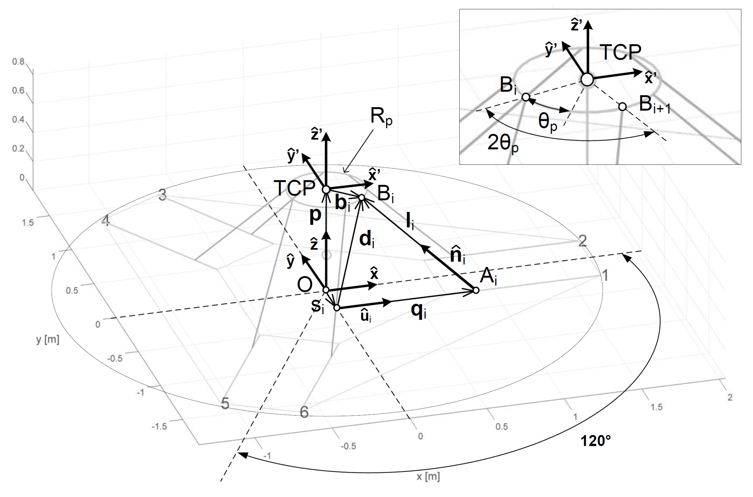
The Hexaslide architecture can be analysed taking into consideration the following parameters (Figure 4) for the optimization process:
- s: semi-distance between two parallel guides;
- : length of the links;
- : radius of the circumference on which the platform joint centres are located;
- : semi-angular aperture between the two segments connecting the origin of the Tool Center Point (TCP) reference frame and a couple of platform joints;
- : height of the centre of the desired workspace.
For this architecture, the same kinematic chain is replicated identically for six times.
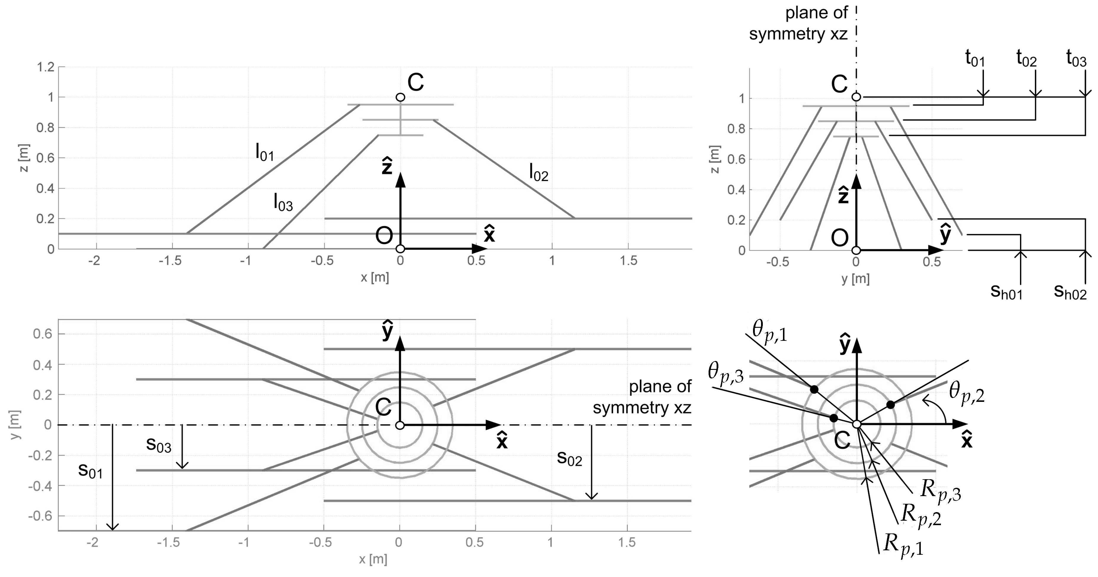
The Hexaglide architecture, shown in Figure 5, can be analysed considering a higher number of parameters because three different kinematic chains can be identified in the robot configuration. The parameters to be optimized are:
- : radius of the circumference on which the platform joints 1 and 2 are located;
- : radius of the circumference on which the platform joints 3 and 4 are located;
- : radius of the circumference on which the platform joints 5 and 6 are located;
- : semi-angular aperture between the two segments connecting the origin of the TCP reference frame and platform joints 1 and 2;
- : semi-angular aperture between the two segments connecting the origin of the TCP reference frame and platform joints 3 and 4;
- : semi-angular aperture between the two segments connecting the origin of the TCP reference frame and platform joints 5 and 6;
- : vertical distance between TCP and the plane where platform joints 1 and 2 lie;
- : vertical distance between TCP and the plane where platform joints 3 and 4 lie;
- : vertical distance between TCP and the plane where platform joints 5 and 6 lie;
- : length of links 1 and 2;
- : length of links 3 and 4;
- : length of links 5 and 6;
- : semi-distance between parallel guides 1 and 2;
- : semi-distance between parallel guides 3 and 4;
- : semi-distance between parallel guides 5 and 6;
- , : vertical distance between ground and parallel guides;
- : height of the center of the desired workspace.
For this architecture, each kinematic chain is replicated twice, one on both sides of the longitudinal median plain of symmetry.
The goal is to optimize robot kinematic performance while ensuring the desired workspace boundaries. In order to define a proper objective function, the desired workspace is discretized in elementary volumes: for each elementary volume, the specific set of parameters under analysis must be allowed to reach its centre point. Moreover, for each centre point analysed, the resulting machine must be able to orientate the TCP with any possible combination of pitch, roll and jaw angles varying inside a predefined range. If that is not the case, the elementary volume is added to the total volume that the current set of parameters is not able to cover. In order to make the computational cost affordable and restrict the checks to a finite amount of angles combinations, the three angular ranges are discretized. The evaluation of the objective-function is performed firstly by fixing the mobile-platform orientation , and thereafter computing the part of volume that end-effector is unable to reach for these specific orientations, such as:
where the combination of parameters i, j, k unequivocally identify a check-point of the workspace in which , , represent the number of discretization points, respectively, along the x, y, z axes. The variable is equal to 1 if the specific parameters prevent the end-effector from reaching the pose defined by i, j, k and , and 0, otherwise. The term is the elementary volume resulting from the discretization of the workspace.
This procedure is repeated for all combinations of pitch, roll and jaw angles and the resulting value for the objective-function is computed as:
Even if a volume portion is discarded for only one specific orientation, that portion of workspace is excluded for the corresponding geometrical configuration. Using this approach, in the ideal case in which a set of parameters allows the robot to reach any point in the workspace regardless of its orientation, the objective-function would be equal to 0. On the other hand, if the set of parameters does not allow the reaching of a particular point of the workspace, the objective function would assume a value equal to the dimension of the single discrete volume times the number of orientations for which that volume has been discarded.
The kinematic capability of reaching each point with every possible orientation is not in itself enough, but additional constraint definitions are required. The kinematic constraints are defined as follows:
- Distance between the i-th platform joint and the corresponding base joint should not exceed the length of the link for geometric congruence;
- Each actuated joint coordinate has to be comprised within a range defined by the dimension of the machine, since actuators’ stroke range have a direct impact on the major bulk direction of the machine, longitudinal for the Hexaglide, and radial for the Hexaslide;
- Each passive joint, both platform and base ones, should respect their respective mobility ranges.
The kinetostatic constraints are defined by the transmission ratio between forces and moments acting on the end-effector and the actuation forces. This transmission ratio for each actuator is computed and the maximum should be lower than a prescribed limit value. As is common for PKMs, this transmission ratio varies considerably within the nominal workspace due to nonlinear kinematics, especially in proximity of the singular configurations. The geometric constraints enforce the respect of the minimum distance between two links and between a link and the mobile platform in order to avoid the problem of self-collision of the component for particular poses.
The solution related to the minimisation of the objective function has been obtained through a single objective genetic algorithm approach [6]. The use of a semi-stochastic search and the evaluation of the performance of different individuals at each iteration makes the process of finding the global minimum of the objective-function to be minimized, easier. The steps characterizing this kind of algorithm are:
- Choice of a sufficiently high number of individuals representing a generation in order to have a significant statistical sample;
- Evaluation of the performance for each individual of the current generation depending on the values assumed by its genes;
- Choice of the group with the better performance that will constitute the elite and will pass unchanged to the next generation;
- Creation of a new generation based on elitary choice, crossover and mutation;
- Computation of the performance of the individuals of the new generation in comparison to the goal desired.
The algorithm would keep modifying parameters trying to cover the desired workspace as much as possible and minimizing the defined objective function. In Table 1 and Table 2, the lower and upper bounds imposed at the beginning of the optimization and the optimal values obtained are reported.
Minimum distance between the links, minimum distance between links and platform, transmission ratio and maximum and minimum strokes of the actuated joint coordinates are mapped throughout the workspace to guide one in the choice of the best architecture. The following conclusions hold respectively for the Hexaslide and Hexaglide.
Hexaslide:
- Topology: both the height and the in plane bulkiness of the manipulator are quite limited. When the robot is in the home position, the links are arranged in such a way that a good compromise is achieved between the capacity to generate velocity in all directions and to bear external forces without too much effort required by the actuators.
- Link-to-link and link-to-platform minimum distances: The link-to-platform minimum distance recorded is above 270 mm throughout the workspace, thus avoiding any risk of collision between the legs.
- Force transmission ratio: the worst case obtained by the computation is closed to the limit value of 5 but restricted to only a few small lower regions of the workspace.
- Actuated joints maximum and minimum stroke: as the joints coordinate distance with respect to the global reference frame is always positive, it is sufficient to check the maximum value in order to evaluate the bulkiness of the robot. This joint coordinate excursion is about 1 m.
Hexaglide
- Topology: The in plane bulkiness of this robot is much higher with respect to the Hexaslide. Moreover, the centre of the desired workspace in the optimized configuration is placed in a higher position compared to the Hexaslide configuration.
- Link-to-link and link-to-platform minimum distances: no risk of self-collision between the elements has been detected.
- Force transmission ratio: the transmission ratio remains limited above 2.5.
- Maximum and minimum stroke: the bulkiness of this solution is higher compared to the Hexaglide one.
It can thus be concluded that Hexaslide architecture is more compact compared to Hexaglide but reaches higher values of force transmission ratio. The Hexaslide architecture has been chosen due to its lower vertical bulkiness, more compact in plane dimensions, better workspace isotropy and lower position of the workspace centre. All of these features make it possible to install the machine under the wind tunnel floor level, reducing the robot influence on the air flow quality and keeping the turbine farther from the wind tunnel ceiling. Moreover, Hexaslide offers two additional advantages: all the elements that make up the links are the same for all six of the kinematic chains and the radial symmetry simplifies the design process. Hereafter, this machine will be referred to as Hexafloat, while the term Hexaslide will refer to the specific architecture of the robot.
2.2. Kinematics Analysis
In order to develop the optimisation problem and design the control algorithm of the robot, it is necessary to solve the inverse and forward kinematics. In this section, for the sake of briefness, only the solution of the inverse and forward kinematic problem of the robot architecture chosen is presented.
2.2.1. Inverse Kinematics (IK)
In order to study Inverse Kinematics, two different reference frames have been considered, the global one and the local one with origin in the TCP and built into the robot platform. With reference to Figure 6, two different vector closures for each kinematic chain can be set up in order to compute the joint coordinates vector q. The first vector closure allows one to determine the absolute position vector of the platform joint with respect to a point that is the intersection of the direction with its orthogonal plane passing through the global origin. Each has a fixed length with different orientations in the - plane:
where is the rotation matrix defining the platform orientation. This matrix is used to transform the expression of , constant into a rotating local reference frame, in its equivalent with respect to a zero orientation local frame translating with the platform. Position vector and the offset complete the transformation from the zero orientation local frame to the global one. The second vector closure allows one to determine the position of the i-th slider on the guide:
The magnitude of vector corresponds to the length of the robot leg while represents the guide direction unitary vector. This procedure is identical, except for the orientation of , and , for all six links of the robot.
2.2.2. Forward Kinematics (FK)
The Hexafloat robot will not be equipped with sensors able to directly measure the platform position and orientation, therefore a good quality FK could work as a virtual sensor for the pose of the robot. A high frequency estimation of the actual pose of the TCP would be a valuable feedback tool for the other controller in the HIL setup, but a short calculation time and overall stability, in the case of numerical algorithms, is crucial. Extensive research has been conducted to ascertain analytical methods to solve the FK of PKMs, especially for Gough–Steward configuration, but the pose of the robot has not been expressed in explicit form so far.
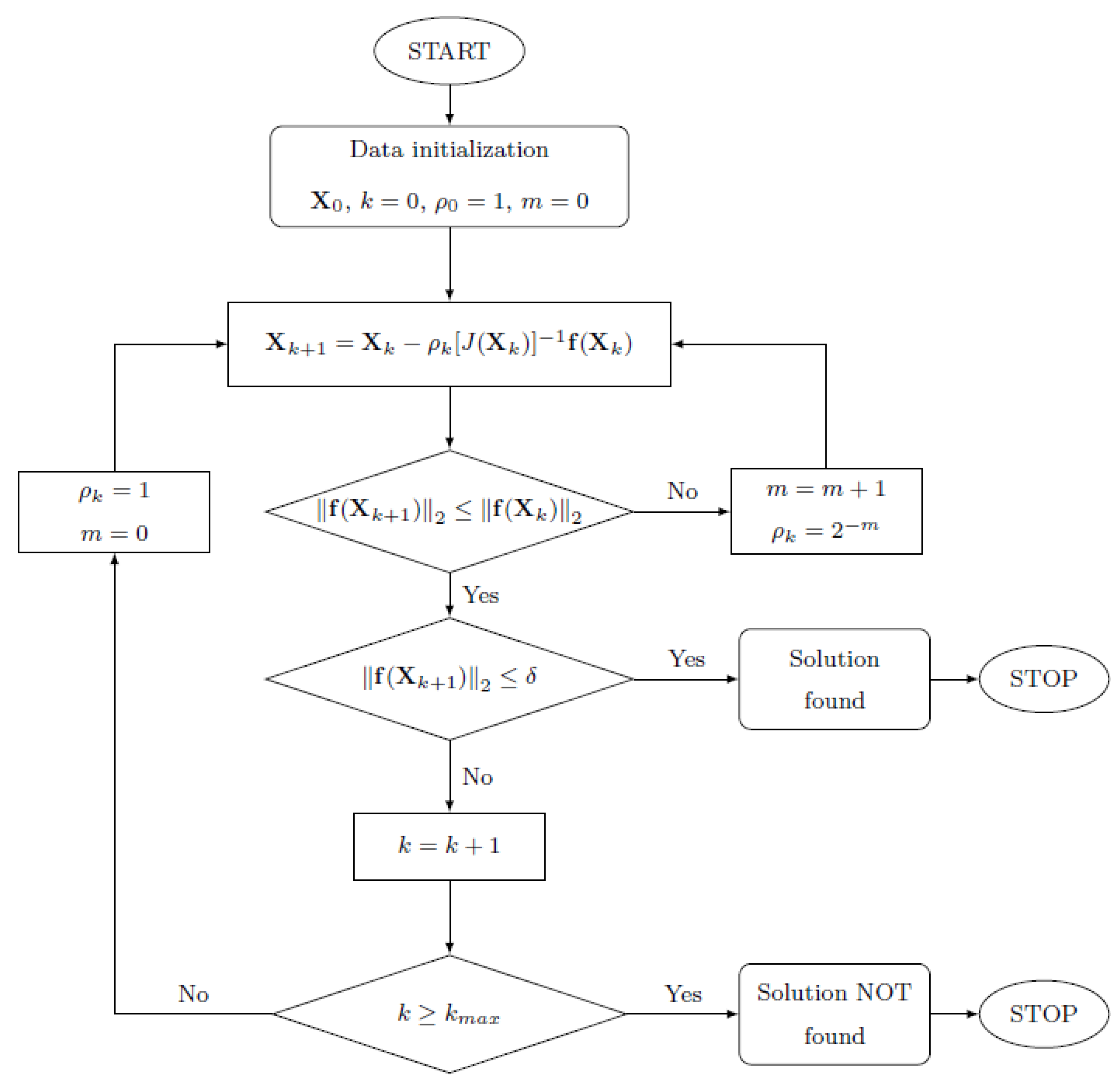
Considering numerical methods, the Newton–Raphson (NR) algorithm has its numerical stability highly dependent on the accuracy of the initial approximation of the solution vector so a monotonic descent operator can be added obtaining the so-called Modified-Global-Newton–Raphson (MGNR) algorithm, able to estimate the FK solution of six-DoF parallel robots for any initial approximation in the non-singular workspace without divergence. The algorithm requires the definition of a system of six nonlinear equations and the evaluation of a matrix of partial derivatives:
The evaluation of partial derivatives matrix can be simplified by implementing Jacobian-Free-Monotonic-Descendent (JFMD) algorithm. A first-order Taylor expansion can be used to approximate the partial derivatives matrix in a numerical way. The JFMD method is implemented via the following steps:
- proper initial approximation of for the solution is chosen and the corresponding is calculated;
- the th solution attempt is calculated according to the following formula:where is the monotonic descent factor. It starts from 1 and during each iteration is calculated as , where m is the number of rechecking times in the corresponding iteration, necessary to obtain the monotonic trend. The approximated Jacobian matrix is evaluated from the first-order Taylor expansion of its partial derivatives and considering a perturbation parameter of 1 × 10. The i-th row and j-th column of the approximated Jacobian matrix is evaluated as:
- convergence criterion is defined imposing the error to satisfy the following inequality:
- the algorithm stops if convergence is achieved or the maximum number of iterations is reached:where is the required computation tolerance and is the given maximum number of iterations.
The first initial approximation must be taken close to the Home Position ( mm from the ground reference frame), where the robot is supposed to be when switched on. For the following times, the initial approximation is chosen as the estimated pose at the previous cycle. The logic of the JFMD algorithm is clarified in the flow chart in Figure 7. Thanks to C language implementation, this routine is able to converge to a solution in relative little iteration, with a mean calculation time of around 50 s in the actual hardware chosen to control the robot. This performance allows one to use FK as a virtual real-time sensor with sufficient accuracy.
2.3. Velocity Analysis and Kinetostatic
In order to determine the relation between the velocity of the TCP and the ones of the joint coordinates, it is necessary to calculate the Jacobian matrix. If all six links are considered together, a compact matrix form coupling the joint velocity vector and the workspace velocity vector w can be defined:
and with some algebraic steps:
The solution of the kinetostatic analysis provides the actuation forces required to bear the external forces applied to the TCP. Due to the virtual work principle and knowing that the virtual variation of the workspace coordinates is related to the virtual variation of the joint coordinates through the Jacobian matrix , the actuation forces can be computed as:
The representation of the way in which forces applied to the robot platform are transmitted to the actuators is obtained considering the unitary hypersphere of forces in the workspace [7]. This unitary hypersphere is transformed into a hyper-ellipsoid in the space of actuation forces. This is a common description used in the robotic field in order to characterise the behaviour of the robot in every point of the working space and it states that, if one of the forces applied to the TCP reaches the maximum value of 1, the other components must be nil. An alternative representation is based on the use of a hyper-cube of unitary semi-side that is transformed into a hyper-polyhedron through the Jacobian matrix, as shown in Figure 8. Moreover, it should be noted that the inverse Jacobian matrix can be split into a translational and a rotational part as presented in [8]. Using this approach, it is possible to note that the rotational components of the inverse Jacobian matrix are dimensional and in fact they correspond to a length. In order to let all the elements of the inverse Jacobian matrix be dimensionless, it is useful to divide the rotational components by a scale factor defined as characteristic length . In this way, a normalized inverse Jacobian matrix is obtained and is used to obtain the maximum actuation force.
3. Actuation Chain Sizing
A proper sizing of mechanical components and actuating systems requires the knowledge of the most power demanding motion that the machine is required to execute, considering the influence of robot dynamics and carried loads. For the application taken into account, the movement of the end effector is unknown in advance because it depends on the wind effect over the wind turbine and the mathematical model used to define the behaviour of the floating structure. To obtain a scenario of the possible movement of the end effector, it is necessary to consider an approximation of the wave motion of the sea expressed by a combination of six cosinusoidal functions [9,10]. Analysing any combination of a parameter set, which is used to define the sea behaviour, one can obtain a possible end effector motion. The time history of the sea level is expressed as:
where is the amplitude, the pulsation, and the phase shift. Both amplitude and phase shift change very slowly in time so it is reasonable to assume they are constant for the whole duration of the simulation and the time history of each DoF is described as:
where is an offset parameter taking into account the initial pose of the robot.
The worst operating conditions may be represented in the case where all frequencies and amplitudes assume their maximum value. However, the intrinsically nonlinear kinematic of the robot may invalidate this assumption. In effect, it is not guaranteed that this is the most demanding case in terms of internal loads, motor torques, velocities and accelerations. Furthermore, a simple co-sinusoidal motion of the end-effector is translated into a periodic motion of the joint coordinates where higher order harmonics with respect to the appear. It is difficult to predict if the energy associated with the higher order harmonics of a specific is bigger than the energy of the harmonics corresponding to a lower .
The four characteristic parameters are thus defined in the following ranges:
- Initial pose : may vary in the range ;
- Frequency : in the range between and ;
- Phase shift : in the range of ;
- Amplitude : its maximum range is and the relation has to be verified to guarantee that the end-effector remains within the boundaries of the desired workspace. The effective range of is obtained by combining the maximum range with the expressed relation, eventually modifying it in the event that is different from zero.
In order to test any pose in the working volume, a procedure has been designed [11]. Firstly, the workspace has been divided into a finite number of portions. For each of these, an admissible range of motion parameters for each degree of freedom has been chosen. In particular, these ranges have to be discretized in order to obtain a finite number of combinations. Therefore, a set of time histories for the six-DoF end-effector is generated and thereafter the inverse kinematic and dynamic problem solved in order to calculate the motor torques required for each set.
3.1. Multibody Model
The procedure described above needs a mathematical model to be implemented. In particular, a multibody model of the robot has been developed using the commercial software MSC ADAMS 2016 in order to compute the dynamic and kinematic quantities that allow one to properly size mechanical components as well as the actuating system [12]. At the preliminary stage of the project, the inertial properties of the components, that make up the robot, are unknown and must be estimated. The results obtained by the use of the multibody model and the developed procedure are used to refine these values and update the model to subsequently enhance the results accuracy and converge towards the final result.
The developed multibody model is based on a parametric approach in order to be easily integrated into the motor sizing procedure. The first step for the model formulation is the definition of a set of reference frames located in positions that allow one to easily define the inertial properties, joints, applied forces and measurements points. The reference frames created are: a TCP reference frame; six reference frames called in correspondence to the centre of the end-effector joints; six reference frames called in correspondence to the centre of the base universal joints; six reference frames called located at the origin of the guide axes, as shown in Figure 9.
The three main components for each kinematic chain are: platform, links and sliders. The element called platform takes into account the mobile platform, the six spherical joints attached to it, the six axes load cell used to measure the forces and moments exerted by the scaled model of the turbine on the robot. Due to the symmetry, the centre of mass is expected to be located on the z-axis of the TCP reference frame and the principal axes of inertia are expected to be parallel to the axes of the TCP. Links can be represented as cylinders whose centre of mass is located in the middle of the link and whose principal axes of inertia are aligned with those of the reference frame. The elements called sliders take into account the universal joints, joint supports and sliders of the transmission unit. Since these bodies will be subjected to a purely translational motion during simulations, it is sufficient to characterise them with their total mass. This schematization with the equivalent mass and inertial properties of the assembly is possible because the model described in this section is supposed to be rigid. The mechanical and geometrical limits of each joint are represented by locking one or more relative degrees of freedom and giving a limited range of displacement/rotation among the possible ones.
3.2. Monte Carlo Method
Due to the impossibility in the definition of the most demanding task for this application, a statistical approach has been developed, based on the Monte-Carlo Method. This novel approach is implemented as follows:
- Choice of a sufficiently high number M of simulations, each of which has a specific time history for every DoF.
- Definition of the Probability Density Functions (PDF) of the input parameters that define every motion task: it is assumed that, at the initial instant, the TCP may be located with the same probability in any point of the workspace. The PDFs chosen for the parameters describing the motion are respectively: for the initial pose a uniform distribution, for the frequency a uniform distribution, for phase shift a uniform distribution and for the amplitude a Rayleigh distribution.
- Repeated sampling of the chosen PDFs: each parameter is allocated a random value for each simulation. The result is a set of M vectors fully defining a six-DoF motion task to be assigned to the TCP.
- Solution of the IK problem to find the joint coordinates time histories to be used as inputs for the simulations involving the multibody model.
- Solution of the inverse dynamics problem for each of the M simulations.
- Post-processing: evaluation of a distribution among the M simulations of the parameters of interest.
The results collected are used to size the mechanical components and the actuators. In particular, it is possible to obtain the slider velocity and acceleration, forces exerted by the motors on the sliders, axial forces along the guide and the so-called “Load factor” for the actuator sizing procedure. A summary set of values is required in order to easily compare these quantities with the corresponding limits specified by the manufacturers. These sets are computed through the extraction of the maximum values for each simulation stored in M array; among these, the highest value is extracted. Therefore, the interval from 0 to the highest extracted value is divided into subranges, and, for each of these, the number of occurrences of the M values is assessed. A set of discrete PDFs is obtained and this represents the probability that the maximum value obtained during a simulation is comprised within a certain interval.
3.3. Actuating System Sizing Procedure
The selection of an actuating system requires one to choose both the electric motor and the gearbox unit. In scientific literature, several procedures to size the motor reducer group are available. In this work, the approach proposed in [11,13] is applied. Independently from the procedure used, the motor reducer sizing is based on the checking of the following three relationships:
- Limit on maximum torque:
- Limits on nominal torque:
- Limit on maximum speed:
is the motor torque, the maximum torque the motor is able to generate, and is the maximum torque that the transmission unit is able to bear. In addition, represents the resistant speed computed on the load side, is the maximum speed the motor can reach without damaging its mechanical components, is the maximum speed the slider can achieve without damaging mechanical components. Following the [13] approach, from the power balance and the thermal check inequality, it is possible to define the transmission ratio as follows:
where the acceleration factor and the load factor are defined as:
The RMS values of torque and acceleration are defined as:
The acceleration factor is a motor characteristic that can be evaluated directly from the datasheets, whereas the load factor depends on the task performed by the actuations system, and, for the case under study, can be calculated using the multibody model. Following the sizing procedure, firstly, the optimal transmission ratio value is evaluated. Then, this value is compared to the transmission ratio purchasable in the market and the closest is chosen taking into consideration that it is within the available range. In particular, greater attention must be paid to evaluate the maximum velocity required during the task and the relative limit transmission value using the formula:
All the results obtained from the multibody simulations refer to the kinematic and dynamic quantities of the manipulator sliders. In order to transform force into torque and linear velocity or acceleration into angular ones, the following equations have to be used:
It is worth noticing that to increase the transmission stiffness and achieve the maximum velocity required, every linear axis of the robot is made up of only a single reduction stage. In particular, the motor is directly connected to the screw by means of a rigid joint and the transmission ratio is the screw lead. Due to the high dynamic performance, stiffness and precision required, recirculating ball screws have been chosen. The double slider configuration for each guide has been selected in order to guarantee a uniform load distribution. The manufacturer’s instructions to correctly size these devices have been followed, in particular to the total length of the screw, maximum allowed velocities, forces that the guide can bear and the like. All of this is summarized in Table 3. As concerns the electric motor OMRON (Tokyo, Japan), as well as the heat dissipation check, the maximum torque achievable has been evaluated.
Figure 10 and Figure 11 show the maximum torque distribution and maximum rotation speed obtained during simulations. Once fixed a coverage threshold, the corresponding values are extracted and they are used as guidelines in the components’ choice. The most restricting limit is imposed by transmission units: the Rollon ballscrew drive (Vimercate (MB), Italy) chosen satisfies the maximum torque test in of the cases with Rayleigh approach and in with the other one. Even if the coverage is not , the choice has been made to find a suitable trade-off between performances and size. As for maximum torque analysis, the most restricting limit for rotation speed is imposed by the linear transmission unit, but, since the selected transmission satisfies more than of the cases, this test is passed.
4. Mechanical Design and Component Sizing
A design process is always iterative: an initial model, which satisfies the preliminary parameters required, is firstly created, thereafter each part of this model is refined and improved in order to enhance its dynamic characteristics and reduce mass and costs of the whole system. In this process, the multibody model plays an important role: it is used many times in an iterative way to analyse the dynamic behaviour of the system after every single modification in order to check the mechanical components and actuation system. For the development of a simulator, it is necessary to realize two kinds of structural analyses: the first one is a static analysis for which the focus is to determine the stress and strain of any mechanical components. The second analysis is a dynamic one performed to obtain the modal behaviour of the system.
4.1. Robot Description and Overview
In order to clarify the results obtained with static and dynamic analysis, a complete overview of the “as built” project is necessary, Figure 12a. The entire system can be divided into two main parts: the Hexafloat manipulator and the auxiliary systems. The first part is made up of “Grounded elements” (all the fixed supporting structure and the power and actuation units), “Joints”, “Links” and “Platform”, whereas the auxiliary systems include: “Lifting system” (a tool used to manage the rest task of the system), “Energy chain” (device that houses cables and the like) and “External Sensors” (sensors for monitoring the system during the operating tasks).
Hereafter is a more detailed description of every component and technical solution adopted.
4.1.1. Grounded Components
This is the framework and gives stability to all the moving parts, Figure 12b. The linear actuation systems are fixed onto it. Therefore, this assembly should be stiff enough to bear static and dynamic loads. The Central plate, made of aluminium, is used to provide the correct orientation and position of the linear guides through calibrated machining. The linear actuators are grouped into two by two and each couple is oriented with an angle of 120 with respect to the other. This leads to a radial symmetry of the machine. Each couple of linear actuators is fixed to the Central plate. To provide further stiffness to the system, avoid undesired tilting and relative displacement between the two couples of guides, three “K” links constrain the Central plate with the “C” shaped supports over which the actuation system is mounted. Aluminium joint holders are used to couple the Joints with the linear actuators. Through the optimization process and the solving of the kinematic closure equations, when the robot is in the Home Position, the direction of each Link is defined and the Joints holder shape and inclination designed. The whole framework will be placed in the wind tunnel using 22 levelling elements to distribute the weight uniformly and maintain the guides on the same plane, without misalignments.
4.1.2. Joints
The PUS kinematic chain on the basis of which the manipulator is realized is made up of an actuated prismatic joint followed by a double revolute joint (universal joint) and a spherical one mounted on the Platform. Placing a universal joint and a revolute one so that the rotation axis of the latter passes through the intersection of the universal joint rotation axes, it is possible to obtain the same numbers of DoFs that the spherical joint has. Therefore, the same universal joint used in the lower part of the kinematic chain is mounted on the Platform, and the rotational degree of freedom is directly realized within the Link. In order to obtain the stiffness, precision and mobility required, a custom joint solution has been realized and they are shown in Figure 13a,b. The main feature of such Joint is the possibility to have a cone shaped motion range with a semi-angular aperture of 45 around the normal direction, designed and assembled to have zero backlash.
Each joint is made up of a couple of Half shells connected to an Inner block through two roller bearings and two Support shafts. These components are tightened by two screws and aligned by two calibrated dowel pins. In this way, the Inner block has a relative movement with respect to the shell, the further DoF is provided by another two roller bearings that support the Inner shaft pinned to the link. All these inner components are packed through a Distance ring and a Closing ring. Half shells and Inner block are made of aluminium, while other components are made of steel. The Joint is fixed to the Joints holder through four screws and aligned with two calibrated dowel pins.
4.1.3. Links
The Links, Figure 14, connect the mobile platform to the fixed one. These bear the pay load made up of the mobile platform, RUAG (RUAG Aviation - Aerodynamic, Schiltwald, Switzerland) load cell, scaled wind turbine and sensors. The RUAG six-DOF weight scale, model W192–6I, is dimensioned for the following forces and moments: N, N, N, Nm, Nm and Nm. Due to the complexity of this device, it is necessary to use a calibration matrix capable of taking into account not only the weight scale deformation but also the working temperature. This calibration matrix, provided by the manufacturer, follows quality procedures in use at the wind tunnel and it is available at the internet address of the Life50+ project. The Link is composed of:
- Lower rod, made of steel, at one side, directly connected to the Inner shaft of the Joint assembled on the grounded components, the other side is used to pack up the bearing group between a mechanical stop and nuts;
- Bearing case, made of steel, which houses the bearings that provide the rotational DoF along the Link axis, and is connected to the Leg pipe by six screws;
- Leg pipe, a hollow cylinder made of aluminium;
- Distance washer, made of steel, it allows the regulation of the total Link length through a threaded connection with the Upper rod. It is also connected to the Leg pipe by six screws;
- Upper rod, made of steel, the final component connected to the Inner shaft of the Joint assembled on the Platform;
4.1.4. Platform
The Platform, Figure 15a, is realised in order to define the right position of the joints and the six-DOF weight scale. It is made up of the following elements:
- Bottom plate, made of aluminium, necessary to sustain and distribute the load and it is the frame of the Platform;
- Three Angular joints holder, made of aluminium, needed to guarantee the correct orientation angle of the Joints;
- Top plate, made of carbon fibres, to give added rigidity to the structure;
- RUAG 6-axis load cell, to measure loads exchanged between the machine and the wind turbine.
4.1.5. Auxiliary System
Two auxiliary systems have been designed: an Energy chain (Figure 15b) and a Lifting system (Figure 16b). The Hexafloat machine is designed to stay below the floor of the wind tunnel when not in operation. In this configuration, the machine has to overcome a singularity to reach Home Position and a Lifting system helps the robot to pass this critical point in the rise and return phases. This system can be schematically modelled as in Figure 16a as an isosceles three-hinged arc, in which hinge A is placed on ground, B on the Moving carriage and C at the central part of the Three points beam, thus allowing a vertical movement of the Three points beam top end (point D). Furthermore, a four-link mechanism is coupled to this system in order to keep it parallel to the ground along the whole stroke of the Coupling platform, mounted on top of the lifting mechanism. The Moving carriage is driven by the motor through a trapezoidal screw, which converts motion from angular to linear.
Measuring and actuation devices will be mounted on the Platform and on-board the scaled wind turbine, and these instruments need to be fed by electric energy and have to be connected to a controller in order to guarantee a real-time data exchange. Therefore, a cable housing system is needed in order to protect cables, maintain a good flexibility while following the Platform movements, without interfering with these. The system is made up of the following elements: four “L” plates supports, made of steel; two lateral connecting plates, made of aluminium; two mounting brackets with strain relief mounted, respectively, on the Platform and on Parts on ground; an intermediate mounting bracket; a mounting sliding bracket and a flexible chain.
4.2. Static Analysis
Through the results obtained from the multibody analysis, one can determine the most critical load acting on the system. In particular, the interest is on the force that must be borne by the links because, through this, the remaining parts of the system are loaded. For safety reasons, an overestimated value of 2500 N is assumed both in traction and compression for every link. The static analysis has been performed using a commercial FEM solution and several models have been studied in order to take into consideration both single elements and their subassembly. Taking into account the final configuration, one can state:
- Grounded components: The symmetry of the assembly allows one to take into account only one third of the frame. Moreover, only the aluminium profile of the linear actuator is taken into account because it bears the vertical loads. A “worst” vertical load (i.e., 2500 N) is applied on each guide and positioned with different combinations of the total actual stroke of the sliders (i.e., 0%, 25%, 50%, 75%, 100%). Local stresses and strains never exceed the limit values, Figure 17a.
- Joint: bearings have been substituted with rigid components to simplify the assessment. Different configurations of angle are tested both as regards compression and traction with an applied load of 2500 N, Figure 18a,b. Only the rod shows visible deformations and stresses. In order to better investigate the behaviour of internal components, other analyses have been carried out and no problems have been reported by the results:
- −
- Inner Block: a load of 2500 N is split into two equal loads, each one acting on a set of bearings. Maximum stress registered is 85 MPa, which is far below the admissible stress of 250 MPa, Figure 19a.
- −
- Support shaft: a load of 1250 N is applied for simulating the presence of two Support blocks per Joint. The test is effected by loading one end of the shaft and maintaining the other one fixed, Figure 19b.
- −
- Inner shaft: a load of 2500 N is applied in the midspan and both ends are pinned in order to simulate the presence of the two bearings, Figure 20a.
- Platform: two horizontal forces are applied at different heights on the TCP. The first of 200 N located at 1.0 m and the second of 100 N at 1.5 m corresponding, respectively, to equivalent inertial load and aerodynamic thrust due to the pay load. These loads are borne very well by the structure both in terms of stress and displacement, Figure 17b.
- Lifting system: this device has to generate a total lift of 150 mm in a time span of about 15 s with a cycloidal motion curve and must also bear the weight of all the moving parts of the robot. This system has been developed in order to help the robot to overcome the singularity configuration during the start and stop procedures. The analysis reveals maximum values occurrence at the initial phase of the rise and FEM analysis ensures that stress remains below the critical values.
4.3. Purchased Components’ Sizing
Final choices regarding motors, linear actuators and the energy chain are listed.
4.3.1. Motors
The selected model is the OMRON R88M-K2K030F-BS2, whose main characteristics are collected in Table 4(a). The Lifting system motor, required to bear the torque increment given by the low efficiency of the trapezoidal screw adopted, is the OMRON R88M-K20030T-BS2, the main characteristics of which are reported in Table 4(b). Both motor models have an auxiliary brake for safety reasons and an encoder to allow one to have a control of position and velocity. For the 2 KW motor of the robot, the encoder is a quadrature incremental encoder with a maximum resolution of 4,194,304 cnt/rev.
The encoder signal is processed in order to obtain a lower resolution of 131,072 cnt/rev. The resulting linear resolution of 3,276,800 cnt/m is obtained considering a lead of 0.04 m/rev for the ball-screw linear axis. For the lifting system motor, the maximum encoder resolution is 131,072 cnt/rev. The modified used resolution is of 13,107.2 cnt/rev, thus obtaining the same linear resolution of the robots axis due to a smaller lead of 0.004 m/rev.
4.3.2. Linear Actuator
The linear actuator chosen is the model TH145 SP4, produced by ROLLON and whose characteristics are reported in Table 5(a). The following customizations are required: screw lead of 40 mm per revolute, to allow the respecting of required performances; two calibrated centring holes on its lower side to correctly assemble the central plate; two calibrated centring holes on the external carriage to allow the correct positioning of the Joint holder.
4.3.3. Other Components
The selected energy chain is Igus (Colonia, Germany) Riflex TRE.40 whose main characteristics are reported in Table 5(b). Tapered roller bearings chosen both for the links and joints are the INA FAG 30202-A. These support both axial and radial loads, thus avoiding the usage of more than one bearing. KTR-TOOLFLEX20M motor coupling is chosen. Due to the reduced space available for the Lifting system, a more compact model of bearing INA FAG 3000-B-2RS-TVH has been chosen. It is a double row angular contact ball bearing, which can bear both axial and radial loads. KTR Rotex 19/92Sh-A/2.1-11/2.0-8 motor coupling has been chosen for the Lifting system and it provides the required performance and encumbrance constraints.
4.4. Modal Analysis
In this section, the approach followed to assess the correctness of the overall design, in terms of dynamic behaviour, is reported. More specifically, the goal is to verify that the first normal modes of the coupled structure coincide with those of the turbine only, in order to minimize the dynamic effects of the robot. Nevertheless, the modal behaviour of a robot strongly depends on the specific pose of the end effector, since the mass and stiffness distribution change according to the pose.
The normal modes and their associated frequencies are computed in order to verify that the frequencies in the first normal mode were high enough. In particular, they must be higher than the well defined frequency range for all the robot poses in to the working volume. The frequency range depends on the dynamic behaviour of the scaled turbine.
To analyse the dynamic response of the manipulator, the entire workspace was discretized, and the trend of the frequency corresponding to the first normal mode over the entire workspace was mapped on specific planes that intersect the robot workspace. The procedure is listed below:
- Identification of planes that intersect the workspace.
- Identification of a grid of equally spaced points on each plane.
- Discretization of pitch, roll and yaw angles describing the end-effector orientation:
- −
- Three roll angles: −5, 0, +5,
- −
- Five pitch angles: −8, −4, 0, +4, +8,
- −
- Three yaw angles: −3, 0, +3.
- Modification of the pose of the robot in order to have the end-effector placed in correspondence to each point of the grid and exploring all the possible orientations.
- In correspondence to each pose, linearization of the flexible virtual model and computation of the frequency associated to the first normal mode.
- For each point of the grid, recording the lowest value of frequency among the ones obtained by changing the orientation angles.
The final result is a set of maps, one for each intersecting plane, which show the trend of the lowest frequencies regardless of the orientation of the robot, as shown in Figure 22. To perform these sets of simulations, a simplified design of the robot was created. Lower simplified joints are tied to the ground applying spherical pins and the simulation provides the first three eigenmode frequencies. Links can be regarded as the main cause for a possible deterioration of the behaviour of the coupled system. The main deformations are concentrated on links and an advanced multibody model has been developed in the “Adams” environment, Figure 23, whose links are made of two extremity elements and an intermediate one characterised by aluminium properties. The results given by the two numerical environments are reported in Table 6.
A frequency response analysis has been performed on the wind turbine and on the coupled system made by the wind turbine and the Hexaslide. The aim of this simulation is to check the Hexaslide is not influencing the frequencies of the turbine’s mode of vibrating, thus making the presence of Hexaslide negligible at least from a mechanical point of view.
A swept sine load of 100 N amplitude between 0.1 Hz and 250 Hz has been applied to the rotor centre in wind (x) direction and the displacements and rotation have been measured. This Force is able to well excite the first and most relevant eigenmodes of the turbine.
The results are reported in Figure 24. The first two wind turbine eigenfrequencies are preserved even in the coupled system, while two peaks appear between 75 Hz and 100 Hz.
It can be concluded that, in the range of 0–60 Hz, a robot’s dynamics does not influence the turbine eigenfrequencies.
5. Control Architecture and Electronics
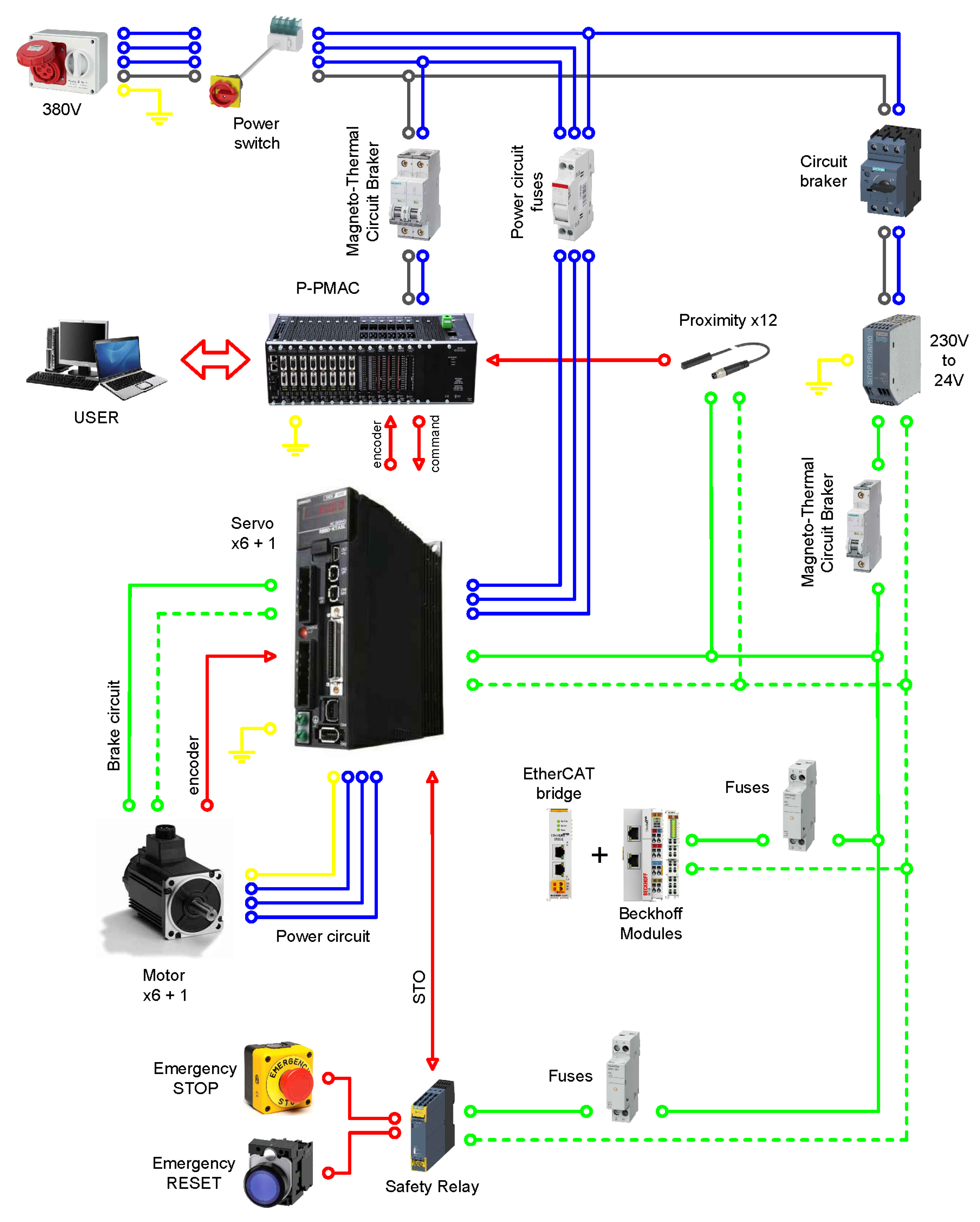
A simplified scheme of the electric panel configuration is reported in Figure 25. The core of the electrical panel is represented by Power PMAC, the property of Delta Tau Data Systems (Chatsworth, CA, USA). There are essentially two zones: one with AC voltage, represented by solid black and blue lines, powered by a 380 V AC line and brings it to the Power PMAC fed at 230 V and to the power circuits of the servo amplifiers fed at 380 V, and the other one with 24 V DC voltage, downstream of the 24 V power supply, which is represented by the solid and dashed green lines. This circuit provides power to the safety relay, limit switches and proximity sensors and to the Beckhoff modules for Ether-CAT communications. Red lines represent the transmission of data between different components.
- EtherCAT modules: the Beckhoff EtherCAT module EK1100 is connected to two EL1008 modules, each of them providing eight digital inputs, and to one EL2008 module that makes available eight digital outputs.
- Servo amplifiers: their main function is to power the motors according to the signals coming from the motion controller. They also process and gather the feedback signals of the motors’ encoders to bring them to Power PMAC. Both signals are transported to and from the servo amplifier into a single cable that is then split into an actual terminal board to be brought to the correct connectors of Power PMAC. Each servo amplifier has the main task of closing the current and phase commutation feedback loop for the motor, starting from the torque reference provided by the Power PMAC motion controller.
- Power PMAC: this is the core of the electrical architecture, it is a general-purpose embedded computer with a built-in motion and machine-control application. It also provides a wide variety of hardware machine interface circuits that allow the connection to common servo and stepper drives, feedback sensors, and analogue and digital I/O points.
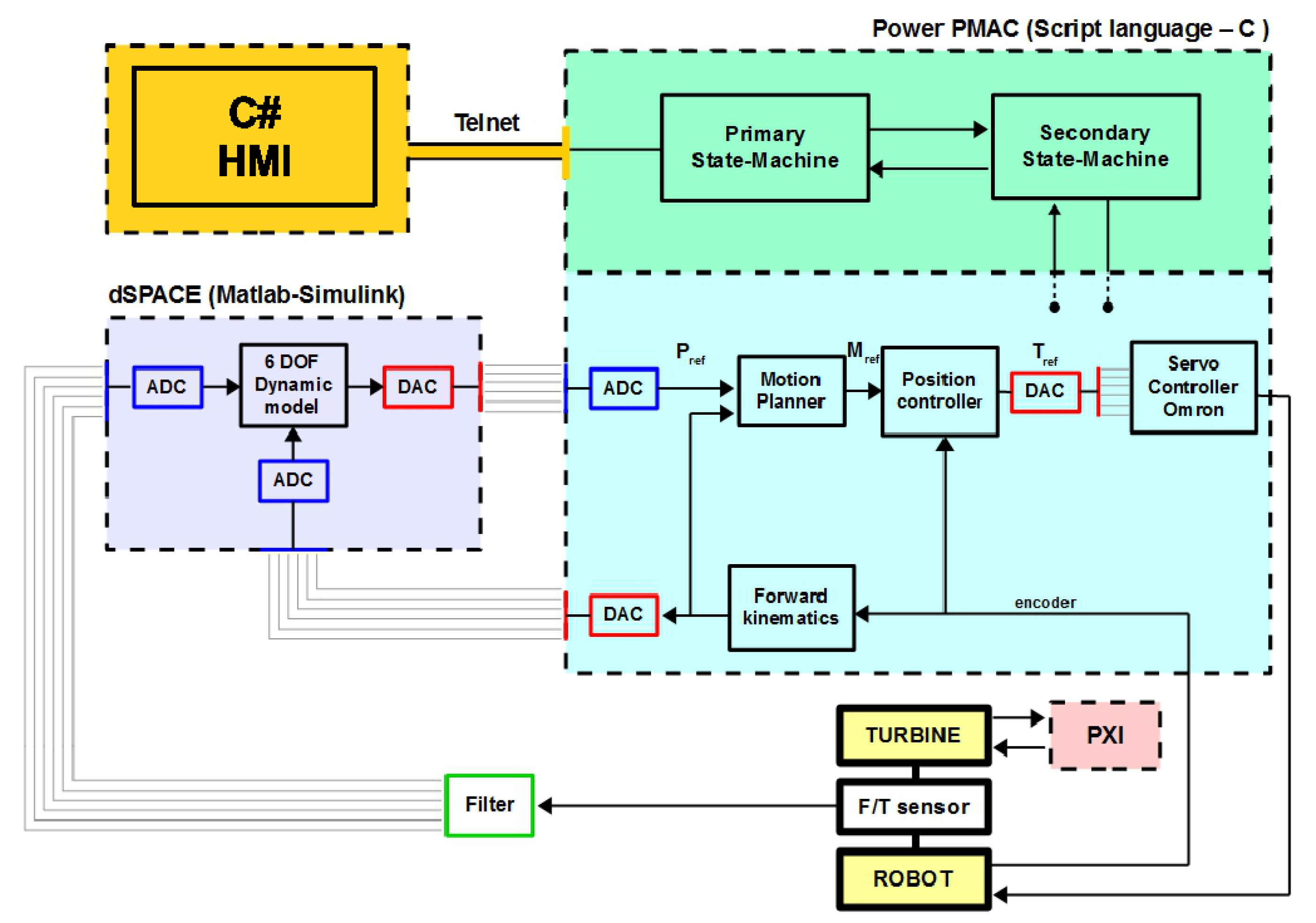
The modular rack is the most flexible configuration, since it permits the user to choose which CPU card, digital or analogue I/O card, axis interface cards and the like to use in the system. Power PMAC can handle all of the tasks required for machine control, constantly switching back and forth between the different tasks thousands of times per second. On this powerful controller, the main control software of the robot has been designed and implemented. Figure 26 shows the general overview of the software architecture. In particular, it is structured so that a primary and a secondary states machine manages the principal functionality of the system, among which the management of the logic state (start, stop, homing, jog, and the like) and the functioning of the machine (managing exceptions, motion programs, debug towards the user). The Position-Based-Admittance-Control (PBAC) control scheme used to close the position loop is highlighted in light blue. Further details in this regard are set out in [14].
The lowest level of the control is constituted by the position and velocity servo loops, giving the analogic torque output reference for the seven servo actuator. Each high level control modality developed has been designed to respect real-time performances desired as well as safety, using advanced tools such as position based admittance control, buffering with time-based control, motion look-ahead for smooth blending, fast C written nonlinear FK and demanding algebra, workspace boundaries check with controlled dynamics on the limits [15], and acceleration saturation with workspace reference tracking check. For more details about control architecture and algorithms, refer to [14,15].
The Human–Machine Interface (HMI) designed allows full control by the user of every significant functioning parameter, simplifying state change and enhancing safety. The HMI communicates with Power PMAC by means of Telnet communication protocol and is completely written in C# language.
6. Conclusions
The experimental verification of the dynamic response of the robot is currently being finalized. The main control features have been tested on a scaled model of the manipulator with optimum results [14,15]. The full scale is now fully operative and its behaviour is under test. For the sake of completeness in Figure 27, the full scale system equipped with accelerometers during the modal analysis campaign is reported. From the first broad results, it appears confirmed that the robot will not interfere, from a dynamic point of view, with the wind turbine scale model [3].
Further experimental modal analysis is staged for the next months, to fully explore the performances not only of the complete mechanical system, but of the whole machine under control influence. First verifications of control performances have already given satisfying results, but further refinement is done every day to an optimized controlled system behaviour in every required operative condition.
This paper shows the design methodology of the HexaFloat system, a six-DoF robot for wind tunnel hybrid testing of floating offshore wind turbines. This setup consists of a parallel kinematic robot, “HexaFloat”, designed and developed to test the dynamics of floating offshore wind turbine concepts, selected within LIFES50+ project, at the Politecnico di Milano wind tunnel, through a hybrid methodology which combines HIL, in real-time measurements (i.e., aerodynamic forces on the wind turbine scale model) and computations (i.e., hydrodynamic forces on platform). This represents the complementary test approach, with respect to the one developed at the Sintef Ocean basin. The final test campaign for LIFES50+ project is staged for July 2018. The complete HIL setup is currently under testing for performance verification, disturbance influence analysis, control of final refinements and tuning and controllers’ communication optimization.
Author Contributions
H.G. and F.L.M. conceived the devices and the sizing tools used; G.R. and M.P. designed the system; F.L.M. developed the control software of the devices; F.L.M., tested the system. H.G. and F.L.M. wrote wrote the paper.
Funding
This project has received funding from the European Union’s Horizon 2020 research and innovation programme under Grant agreement No. 640741.
Conflicts of Interest
The authors declare no conflict of interest. The founding sponsors had no role in the design of the study; in the collection, analyses, or interpretation of data; in the writing of the manuscript, and in the decision to publish the results.
References
- Sauder, T.; Chabaud, V.; Thys, M.; Bachynski, E.E.; Sæther, L.O. Real-time hybrid model testing of a braceless semi-submersible wind turbine: Part I—The hybrid approach. In Proceedings of the 2016 35th International Conference on Ocean, Offshore and Arctic Engineering, Madrid, Spain, 17–22 June 2016; American Society of Mechanical Engineers: New York, NY, USA, 2016; p. V006T09A039. [Google Scholar]
- Bayati, I.; Belloli, M.; Ferrari, D.; Fossati, F.; Giberti, H. Design of a 6-DoF robotic platform for wind tunnel tests of floating wind turbines. Energy Procedia 2014, 53, 313–323. [Google Scholar] [CrossRef]
- Bayati, I.; Belloli, M.; Bernini, L.; Giberti, H.; Zasso, A. Scale model technology for floating offshore wind turbines. IET Renew. Power Gener. 2017, 11, 1120–1126. [Google Scholar] [CrossRef]
- Giberti, H.; Ferrari, D. A novel hardware-in-the-loop device for floating offshore wind turbines and sailing boats. Mech. Mach. Theory 2015, 85, 82–105. [Google Scholar] [CrossRef]
- Fiore, E.; Giberti, H. Optimization and comparison between two 6-DoF parallel kinematic machines for HIL simulations in wind tunnel. MATEC Web Conf. 2016, 45, 04012. [Google Scholar] [CrossRef] [Green Version]
- Ferrari, D.; Giberti, H. A genetic algorithm approach to the kinematic synthesis of a 6-DoF parallel manipulator. In Proceedings of the 2014 IEEE Conference on Control Applications (CCA), Juan Les Antibes, France, 8–10 October 2014; pp. 222–227. [Google Scholar]
- Merlet, J. Jacobian, manipulability, condition number, and accuracy of parallel robots. J. Mech. Des. 2006, 128, 199–206. [Google Scholar] [CrossRef]
- Legnani, G.; Tosi, D.; Fassi, I.; Giberti, H.; Cinquemani, S. The “point of isotropy” and other properties of serial and parallel manipulators. Mech. Mach. Theory 2010, 45, 1407–1423. [Google Scholar] [CrossRef]
- Vinje, T. The statistical distribution of wave heights in a random seaway. Appl. Ocean Res. 1989, 11, 143–152. [Google Scholar] [CrossRef]
- Xu, D.; Li, X.; Zhang, L.; Xu, N.; Lu, H. On the distributions of wave periods, wavelengths, and amplitudes in a random wave field. J. Geophys. Res. C 2004, 109. [Google Scholar] [CrossRef] [Green Version]
- Fiore, E.; Giberti, H.; Bonomi, G. An innovative method for sizing actuating systems of manipulators with generic tasks. Mech. Mach. Sci. 2017, 47, 297–305. [Google Scholar] [CrossRef]
- Fiore, E.; Giberti, H.; Ferrari, D. Dynamics modeling and accuracy evaluation of a 6-DoF Hexaslide robot. In Nonlinear Dynamics; Springer: Berlin, Germany, 2016; Volume 1, pp. 473–479. [Google Scholar]
- Giberti, H.; Cinquemani, S.; Legnani, G. A practical approach to the selection of the motor-reducer unit in electric drive systems. Mech. Based Des. Struct. Mach. 2011, 39, 303–319. [Google Scholar] [CrossRef]
- La Mura, F.; Todeschini, G.; Giberti, H. High Performance Motion-Planner Architecture for Hardware-In-the-Loop System Based on Position-Based-Admittance-Control. Robotics 2018, 7, 8. [Google Scholar] [CrossRef]
- La Mura, F.; Romanó, P.; Fiore, E.; Giberti, H. Workspace Limiting Strategy for 6 DOF Force Controlled PKMs Manipulating High Inertia Objects. Robotics 2018, 7, 10. [Google Scholar] [CrossRef]
Figure 1.
General scheme of the HexaFloat design process.

Figure 2.
Dimensional constraints: (a) Workspace constraints; (b) Wind tunnel frontal view and dimensions of the space dedicated to the machine.
Figure 2.
Dimensional constraints: (a) Workspace constraints; (b) Wind tunnel frontal view and dimensions of the space dedicated to the machine.

Figure 3.
Hexaglide robot (a) and Hexaslide robot (b) simplified geometry scheme.

Figure 4.
Hexaslide geometric parameters, the Cartesian space is represented in meters.

Figure 5.
Hexaglide geometric parameters, the Cartesian space is represented in meters.

Figure 6.
Vector closures used to solve the inverse kinematics (IK) problem: in blue, the 1st closure while in red the 2nd one.
Figure 6.
Vector closures used to solve the inverse kinematics (IK) problem: in blue, the 1st closure while in red the 2nd one.

Figure 7.
Flow chart of the Jacobian Free Monotonic Descendent (JFMD) algorithm.

Figure 8.
Transformation of the workspace forces unitary hypercube into the actuation forces hyperpolyhedron.
Figure 8.
Transformation of the workspace forces unitary hypercube into the actuation forces hyperpolyhedron.

Figure 9.
Reference frames configuration, the Cartesian space is represented in meters.

Figure 10.
Maximum torque distribution along all the simulations.

Figure 11.
Maximum angular velocity distribution along all the simulations.

Figure 12.
Components. (a) Hexafloat exploded; (b) parts on the ground partially exploded view.

Figure 13.
Custom joint. (a) joint exploded view; (b) joint assembly.

Figure 14.
Link exploded view.

Figure 15.
Platform and energy chain. (a) platform exploded view; (b) energy chain assembly.

Figure 16.
Lifting system. (a) lifting system scheme; (b) lifting system assembly.

Figure 17.
Movable and fixed platform analysis. (a) parts on ground static analysis; (b) platform static analysis.
Figure 17.
Movable and fixed platform analysis. (a) parts on ground static analysis; (b) platform static analysis.

Figure 18.
Joint analysis. (a) joint static analysis; (b) joint static analysis, inclined configuration.
Figure 18.
Joint analysis. (a) joint static analysis; (b) joint static analysis, inclined configuration.

Figure 19.
Inner block and shaft analysis. (a) inner block static analysis; (b) support shaft static analysis.
Figure 19.
Inner block and shaft analysis. (a) inner block static analysis; (b) support shaft static analysis.

Figure 20.
Inner shaft and link analysis. (a) inner shaft static analysis; (b) link static analysis.
Figure 20.
Inner shaft and link analysis. (a) inner shaft static analysis; (b) link static analysis.

Figure 21.
Lower rod analysis. (a) lower rod compression analysis; (b) lower rod traction analysis.

Figure 22.
Modal frequencies maps.

Figure 23.
Numerical modal analysis. (a) Inventor 1st mode of vibration; (b) Adams 1st mode of vibration.
Figure 23.
Numerical modal analysis. (a) Inventor 1st mode of vibration; (b) Adams 1st mode of vibration.

Figure 24.
Frequency Response analysis of Turbine and Hexaslide with turbine. (a) displacement along direction; (b) rotation around the axis.
Figure 24.
Frequency Response analysis of Turbine and Hexaslide with turbine. (a) displacement along direction; (b) rotation around the axis.


Figure 25.
Simplified scheme of an electrical layout.

Figure 26.
Complete control scheme.

Figure 27.
Hexaslide experimental setup.


Table 1.
Limits and results of the Hexaslide optimization.
| Symbol | Lower Bound | Upper Bound | Optimal Value | MU |
|---|---|---|---|---|
| 400 | 500 | 463.6 | mm | |
| s | 200 | 300 | 203.1 | mm |
| l | 400 | 700 | 686.6 | mm |
| 200 | 250 | 238.7 | mm | |
| 0 | 60 | 38.5 |
Table 2.
Limits and results of the Hexaglide optimization.
| Symbol | Lower Bound | Upper Bound | Optimal Value | MU |
|---|---|---|---|---|
| 500 | 700 | 593.9 | mm | |
| 100 | 980 | 1050.8 | mm | |
| 100 | 980 | 277.7 | mm | |
| 100 | 980 | 330.2 | mm | |
| 600 | 1600 | 1207.7 | mm | |
| 600 | 1600 | 873.9 | mm | |
| 600 | 1600 | 825.7 | mm | |
| 200 | 400 | 306.2 | mm | |
| 200 | 400 | 326.7 | mm | |
| 200 | 400 | 275.9 | mm | |
| −200 | 0 | −183.0 | mm | |
| −200 | 0 | −72.4 | mm | |
| −200 | 0 | 22.9 | mm | |
| 10 | 170 | 77.3 | ||
| 10 | 170 | 37.9 | ||
| 10 | 170 | 100.6 |
Table 3.
Resume of checks done on guides.
| Parameter | Value | Limit Value | UM | |
|---|---|---|---|---|
| Length of the guide | 1100 | > | 650 | mm |
| Max velocity | 1.67 | < | 2.66 | m/s |
| Max acceleration | 28.5 | < | 50 | m/s |
| 1385 | < | 12,250 | N | |
| 1385 | < | 69,600 | N | |
| 1385 | < | 69,600 | N | |
| 174 | < | 3028 | Nm | |
| 174 | < | 2290 | Nm | |
| 174 | < | 2290 | Nm |
Table 4.
Motors’ characteristics.
| (a) OMRON R88M-K2K030F-BS2 Main Characteristics | ||
| Characteristic | Value | MU |
| Tension | 400 | V |
| Nominal Power | 2000 | W |
| Nominal Torque | 6.37 | Nm |
| Maximum Torque | 19.1 | Nm |
| Nominal velocity | 3000 | rpm |
| Maximum velocity | 5000 | rpm |
| (b) OMRON R88M-K20030T-BS2 Main Characteristicss | ||
| Characteristic | Value | MU |
| Tension | 230 | V |
| Nominal Power | 200 | W |
| Nominal Torque | 0.64 | Nm |
| Maximum Torque | 1.91 | Nm |
| Nominal velocity | 3000 | rpm |
| Maximum velocity | 6000 | rpm |
Table 5.
Other components’ characteristics.
| (a) ROLLON TH145 SP4 Main Characteristics | ||
| Characteristic | Value | MU |
| Total length | 1100 | mm |
| Width | 145 | mm |
| Thickness | 85 | mm |
| Screw diameter | 20 | mm |
| Number of charts | 2 | - |
| Total system mass | 30 | kg |
| (b) Igus Triflex TRE.40 Main Characteristics | ||
| Characteristic | Value | MU |
| Total length | 1600 | mm |
| Number of chain links | 116 | - |
| External diameter | 43 | mm |
| Curvature radius | 58 | mm |
| Maximum single cable diameter | 13 | mm |
| Maximum relative rotation | ±10 | |
Table 6.
Eigenmodes frequencies in Home Position.
| (a) Eigenmodes Frequencies Calculated through Inventor | |
| Eigenmode index | Frequency |
| I | 151 Hz |
| II | 154 Hz |
| III | 210 Hz |
| (b) Eigenmodes Frequencies Calculated through Simplified Adams Model | |
| Eigenmode index | Frequency |
| I | 169 Hz |
| II | 171 Hz |
| III | 222 Hz |
© 2018 by the authors. Licensee MDPI, Basel, Switzerland. This article is an open access article distributed under the terms and conditions of the Creative Commons Attribution (CC BY) license (http://creativecommons.org/licenses/by/4.0/).
Share and Cite
MDPI and ACS Style
Giberti, H.; La Mura, F.; Resmini, G.; Parmeggiani, M. Fully Mechatronical Design of an HIL System for Floating Devices. Robotics 2018, 7, 39. https://doi.org/10.3390/robotics7030039
AMA Style
Giberti H, La Mura F, Resmini G, Parmeggiani M. Fully Mechatronical Design of an HIL System for Floating Devices. Robotics. 2018; 7(3):39. https://doi.org/10.3390/robotics7030039
Chicago/Turabian StyleGiberti, Hermes, Francesco La Mura, Gabriele Resmini, and Marco Parmeggiani. 2018. "Fully Mechatronical Design of an HIL System for Floating Devices" Robotics 7, no. 3: 39. https://doi.org/10.3390/robotics7030039
Note that from the first issue of 2016, this journal uses article numbers instead of page numbers. See further details here.