Abstract
Recent advances in planning and control of robot manipulators make an increasing use of optimization-based techniques, such as model predictive control. In this framework, ensuring the feasibility of the online optimal control problem is a key issue. In the case of manipulators with bounded joint positions, velocities, and accelerations, feasibility can be guaranteed by limiting the set of admissible velocities and positions to a viable set. However, this results in the imposition of nonlinear optimization constraints. In this paper, we analyze the feasibility of the optimal control problem and we propose a method to construct a viable convex polyhedral that ensures feasibility of the optimal control problem by means of a given number of linear constraints. Experimental and numerical results on an industrial manipulator show the validity of the proposed approach.
1. Introduction
Robotic systems typically present kinematic and/or dynamic limitations. For example, joint positions are generally bounded within an available range of motion, while actuators implicitly present velocity and acceleration/torque limits. Further constraints can be due to the environment where the robot has to operate (e.g., partial occupation of the robot workspace) or to safety reasons, which may determine velocity and acceleration limitations. Including such constraints in the development of planning and control methods is of utter importance, as their violation might lead to unrealizable motions (with consequent significant errors in the execution of the tasks) or to safety issues (for example, in the case workspace limits are not respected).
Constrained methods are widely diffused, for example, in the case of offline trajectory planning. The general approach consists in the formulation of a constrained optimization problem that should optimize a given objective, such as minimum execution time [1] or minimum energy consumption [2]. This is also the case of global redundancy resolution methods [3], where the robot has to perform an assigned task, and the redundancy can be exploited to optimize a desired objective, such as maximum manipulability [4], dexterity [5], or maximum joint range availability [6]. However, all these methods are typically performed offline as they need the prior knowledge of the task to be performed, and they lead to heavy computational burdens that do not permit their online execution. For this reason, they are not able to handle online trajectory generation and re-planning techniques and this is a relevant limitation, considering recent robotic applications such as collaborative robotics and robots in unstructured environments. To handle the robot constraints in online planning and control methods, optimization-based techniques are becoming more and more widespread as the increasing computing power of modern processors allows their real-time implementation with small sampling periods.
Quadratic programming, for example, is intensively exploited in the resolution of the Inverse Kinematic (IK) problem of redundant manipulators [7,8,9,10,11]. In brief, a manipulator is termed kinematically redundant with respect to a task when it has a number of degrees of freedom greater than the one of the desired task. The IK problem does not present a unique solution, as the transformation between the joint and the task space results in an undetermined system. Such problem is usually addressed at differential level in order to exploit the linear relation between joint and task velocities given by the Jacobian of the robot. This can be formulated as a chain of Quadratic Programs (QP) with decreasing priorities: the tasks are written as cost functions and the robot limits are represented as linear constraints. The possibility of including robot constraints in the QP represents a great advantage with respect to other typical methods (such as the unconstrained projection of secondary tasks in the null space of the Jacobian [12,13]). Further developments in this field explicitly face the problem of possible saturations and task deformations by introducing a scaling variable into the QP to slow down the execution of the tasks if needed [14].
A further improvement of these methods is represented by the use of Model Predictive Control (MPC) techniques, which aim at overcoming issues related to the fact that the previous methods only consider the current state of the robot. In fact, MPC-based methods are able to take into account the future evolution of the system, the tasks, and the constraints, improving the behavior of the robot in terms of task satisfaction and smoothness [15,16]. MPC is also applied to constrained motion planning [17,18] or low-level control applications [19].
Disregarding the particular field of application, a fundamental issue to address when using optimization-based control techniques is the feasibility of the online optimization problem. In fact, feasibility must be ensured in any possible state of the system. Otherwise, a solution to the problem might not exist, and this could cause the algorithm to stop (unless specific but sub-optimal strategies are activated when infeasibility occurs).
Feasibility of the online optimization problem is strictly related to the concept of set viability [20]. A set is said to be viable if, given an initial state within such set, the state trajectory can be kept within the set by means of a proper and realizable input function. In other words, keeping the state within a viable set ensures feasibility for all future time instants. On the contrary, if the state exits the viable set, infeasibility of the control problem will surely occur at a certain time in the future. This is particularly relevant in the case of state-constrained systems, as infeasibility might occur if no viability conditions are added to the control problem but only state and input limits are taken into account.
For robot manipulator control, this issue is common to any control strategy that takes into account both position and acceleration/torque constraints. In this case, the simplistic imposition of box constraints on the position and the acceleration/torque of the robot does not ensure the existence of a feasible solution to the optimization problem. For example, if a robot joint approaches its position limit with high velocity, the position bound will be exceeded due to the bounded admissible deceleration. Few works addressed this issue by means of manually-tuned heuristic strategies that aimed at reducing the velocity of the robot when it approached its position limits [21,22,23]. Many other control strategies did not take into account position bounds, assuming that the reference trajectories were implicitly feasible [24,25]. Notice that the viability guarantee does not ensure the feasibility of the reference trajectory, which could be only verified offline when the whole trajectory is known a priori. Such approach does not apply to online methods, which should be able to handle online trajectory generation and re-planning. In these cases, we can only ensure the feasibility of the optimal control control, which typically aims at minimizing the deviation of the performed motion with respect to the reference trajectory. This means that, although the desired motion might be infeasible, the optimal control problem remains feasible. In this case, a deformation with respect to the nominal trajectory could arise.
A formal viability guarantee was given in [26], which proposed an invariance control scheme for constrained robot manipulators. In particular, viability conditions were derived in order not to exceed workspace limitations with bounded joint accelerations. In [14], a local redundancy resolution technique was proposed: to respect a given deceleration limit in the breaking phase, the position-velocity state region was limited by imposing that the robot was able to stop within the given joint limit (in fact, limiting the state region to a viable set). This approach was similarly adopted in [27] in the context of robust constrained motion planning. Recently, viability for joint-constrained manipulators was explicitly addressed in [28], with a particular focus on the discrete-time implementation of the viability constraints.
All the above-mentioned approaches were based on the derivation of an analytical viability condition for a double integral system with bounded input and output. The resulting condition is quadratic in the velocity state. However, as all the above-mentioned works refer to local/feedback methods, such condition could be easily linearized around the current system state, resulting in variable box constraints on the control actions. However, such linearization is not possible for predictive strategies. In this case, a linear approximation of the viability set should be obtained. For example, Faroni et al. [29] gives a sufficient condition to approximate the quadratic viable set with a linear constraint and maintaining the viability property. Although the approximation technique is easy to implement and does not remarkably increase the computational complexity of the problem, the resulting allowed state region could result to be significantly smaller than the original one.
In this paper, we propose a method to derive a viable convex polyhedron for a robotic system with bounded joint positions, velocities, and accelerations. In particular, a simple optimization problem is set up to determine the maximum polyhedron that approximates the original viable set. The original quadratic condition is approximated by a polyhedron with a given number of sides, by maximizing the area of the allowed velocity-position state-region. Moreover, viability of the resulting set is ensured by imposing that, for all points on the polyhedron boundary, there exists a realizable input action that keeps the next state within the polyhedron itself, which is also demonstrated to be convex and can be therefore rewritten as a linear inequality constraint in optimization-based algorithms (such as linear MPC techniques). The paper shows that, by increasing the number of sides, the polyhedron gives a better approximation of the original viable set, as expected. This means that a larger admissible state region can be exploited by the controller when the resulting constraints are included in the optimization problem. Consequently, the controller can obtain smaller tracking errors when the desired task requires the robot joint to get close to the maximal viable set boundary. In particular, numerical results show the enlargement of the admissible state region as the number of sides increases. Such improvement is more and more evident as the maximum acceleration values gets smaller. Finally, experimental results on a Universal Robots UR10 manipulator demonstrates the validity of the proposed approach. In particular, an MPC algorithm is applied to the tracking problem of a given joint-space trajectory and the results with different viability conditions are compared. Firstly, an experimental example shows that the use of an invariance condition is of vital importance to ensure both the feasibility of the online optimization problem and the satisfaction of the manipulator limits. Secondly, the results show that the viable sets obtained by means of the proposed method permits to obtain smaller (or null) tracking errors in the case the required motion is close to the viability boundary, increasing the performance of the MPC controller.
The paper is organized as follows. Section 2 introduces the concept of set viability applied to constrained kinematic control of robot manipulators. Section 3 illustrates the proposed method for the computation of the optimal viable polyhedron and gives viability and convexity proves. Numerical results demonstrate the effectiveness of the proposed approach in Section 4, while experimental results on a Universal Robot UR10 manipulator are shown in Section 5. Section 6 concludes the paper.
2. Feasibility of the Constrained Kinematic Control Problem
Consider a generic robot joint and denote with q, , its position, velocity, and acceleration, respectively. The limits on q, , and can be therefore expressed as:
where , , , and , , are the minimum and maximum joint position, velocity, and acceleration, respectively.
Assume a discrete-time implementation with sampling period T in which the acceleration is considered as constant along each sampling period. At time k, kinematic limits at the next sampling time can be easily written as linear inequalities in the joint acceleration as:
However, the simplistic imposition of Equations (4)–(6) may result in an empty admissible set, as no feasible solution might exist that satisfies all constraints at the same time [28].
Indeed, the existence of a solution is guaranteed if Equations (4)–(6) are feasible for all the admissible states of the system. This is strictly correlated to the concept of set viability, as mentioned in Section 1. As each joint is modeled as a double integrator, the viability analysis traces back to the viability of a double integrator system with bounded input and output. By imposing the feasibility of Equations (4)–(6), the maximal viability set for the double integrator can be derived analytically [26]. Intuitively, it can be calculated by imposing that, applying the maximum deceleration , the joint stops at with null velocity (). The resulting condition (valid for the upper bound) is given by:
which expresses a quadratic condition in the system states. An analogous condition for the lower bound can be derived likewise.
Such condition can be easily linearized around the current velocity and position, in the case of local methods, as in [14,27]. The inclusion of Equation (7) in the QP ensures that the states of the system (i.e., the joint velocities and positions) remain within a viable set for which the problem is feasible. More details about the discrete implementation in robotic systems can be found in [28].
The necessity of deriving a linear approximation of the original quadratic equation (Equation (7)) comes from the advantages given by the linear formulation in optimization-based controllers (in particular, the significant decrement of computational time and the ease of implementation of linear MPC with respect to the nonlinear one). However, in the case of predictive strategies, the linearization adopted for local methods is not applicable.
To tackle this issue, Faroni et al. [29] proposed a linear viability condition based on a single constraint for each joint. Firstly, it showed that approximating the quadratic constraint in Equation (7) by means of a straight line passing through the extreme points of the maximal viable set (i.e., and the intersection between Equation (7) and in Figure 1) leads to a non-viable set. Then, it derives a linear viability condition by imposing that the maximum deceleration along the linear constraint is exactly equal to the maximum admissible deceleration. In this way, the joint states can be always kept within the resulting set by means of a realizable acceleration. Such condition is given by:
for the upper bound, and likewise for the lower one.
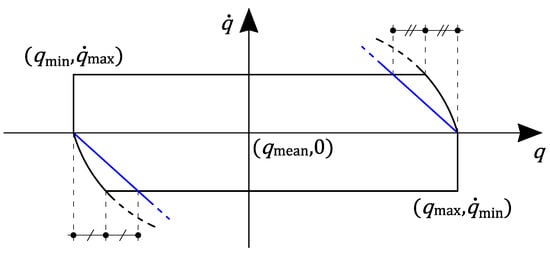
Figure 1.
Viable admissible set for the double integrator system. Black: Maximal region, given by the quadratic inequality in Equation (7). Blue: Conservative linear inequality in Equation (8), as proposed in [29].
Inequalities (Equations (7) and (8)) are graphically represented in Figure 1. Linearity of Equation (8) is a great advantage, as it allows the straightforward inclusion in an optimization problem as a linear constraints. However, it is clear that Equation (8) implies a conservative reduction of the available state-space region compared to Equation (7), and such reduction worsens as the acceleration limits become smaller.
From a practical perspective, the reduction of the admissible state region shows its drawbacks when the robot is required to perform a motion that would violate Equation (8). In fact, the states laying between the linear and the quadratic constraints in Equations (7) and (8) are potentially realizable by the robot, but they are automatically excluded by the controller, with consequent deformation of the desired trajectory. Similarly, for redundant manipulators, shrinking the admissible state region could results in a worse satisfaction of the secondary objectives.
3. Proposed Method
As mentioned in the previous section, viability conditions are fundamental to ensure the feasibility of the control problem. The derivation of linear viability conditions (e.g., Equation (8)) allows their straightforward implementation in an optimization-based control framework, such as MPC algorithms. A strategy to enlarge the admissible region without waving its linearity is therefore proposed. It consists in increasing the number of linear constraints that compose the admissible set. We can therefore state the following problem.
Problem 1.
Given the acceleration, velocity, and configuration limits for each joint, find the maximal viable convex polyhedron determined by a given number of linear inequalities.
We address this problem by converting it into an optimization problem. In particular, for each joint, two optimization problems are set up (one for the upper position bound and one for the lower position bound). Without loss of generality, consider the upper configuration bound for a generic joint (i.e., the first quarter in Figure 1). The optimization variables of the problem are given by the coordinates of the extremes of the segment composing the polyhedron shown in Figure 2. Given a number of segments h, such variables are denoted with the vectors:
whereas a generic point on the polyhedron is denoted with .
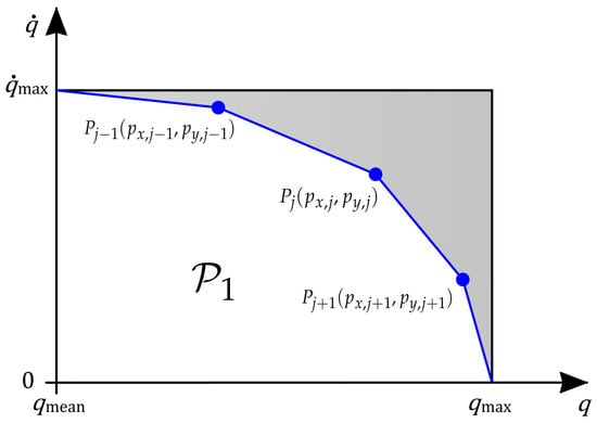
Figure 2.
Construction of the polyhedron .
Now, impose that , where and . To maximize the area covered by the polyhedron, a cost function equivalent to the opposite of such area is defined as follows:
The extremes of the segments are required to lay in the first quarter and have to respect the maximum position and velocity bounds. This results in the following box constraints:
Moreover, as a first necessary condition to the convexity of the polyhedron, we impose:
One last constraint needs to be imposed to ensure that the resulting polyhedron is viable and convex. To this purpose, we resort to a geometrical reasoning. Consider a generic segment whose extremes are the points and and denote with the unitary vector normal to the segment and directed toward the inner region of the polyhedron. It results that:
Consider then a generic point on the segment. By applying the maximum deceleration to the system, the states are forced to move on the curve given by:
The tangent vector to such curve in the -plane is given by:
The vector at is therefore the tangent vector in the point and results to be:
Note that represents the direction of the state movement when the maximum realizable deceleration is applied. The state will therefore be able to remain below the considered segment if the following condition holds:
where denotes the scalar product between two vectors. As
condition in Equation (20) can be imposed on the sole extreme point of each segment and becomes:
Finally, the resulting optimization problem can be written as:
Following the same reasoning, an analogous optimization problem can be set up for the lower position bound. Note that, if the joint limits are symmetric, the solution for the lower bounds can be obtained by “mirroring” the solution of Equation (23) into the third quarter of the -plane. Notice that, as Equation (23) is non-convex, global optimization such as genetic or multi-start algorithms should be adopted to solve the optimization problem (see Section 4).
Denoting with the polyhedron determined by the segments obtained as solution of Equation (23), and with the analogous polyhedron obtained for the lower bounds, the overall polyhedron for the single joint is given by:
Proposition 1.
Polyhedron is a viable set with respect to the given joint position, velocity and acceleration limits. Moreover, such polyhedron is convex.
Proof (Viability)
Viability of the set is implicitly ensured by the imposition of Equation (22). ☐
Proof (Convexity)
To prove it by contradiction, denote the solution of Equation (23) with and assume that the corresponding polyhedron (i.e., the part of the polyhedron in the first quarter) is non-convex. Consider then a triple of consequent extremes , , , which causes a non-convexity. Equations (20) and (21) imply:
Consider now the point given by the projection of onto and denote with the vector normal to . We want to prove that the polyhedron obtained by substituting to in is a feasible and more efficient solution of Equation (23). First, constraints in Equations (12)–(15) are straightforwardly satisfied. Moreover,
as and by construction (where and denote the unitary vectors directed as the horizontal and the vertical axis, respectively).
Moreover, as in Equation (19) is assumed to be negative, the following inequality holds:
Note that Equations (27) and (28) implies that the new candidate solution satisfies Equation (22) and is therefore a feasible solution to Equation (23). Moreover, the candidate solution is more efficient than the assumed one, as
which means that are not the optimal solution of Equation (23), as a feasible and more efficient solution that eliminates such non-convexity exists. Applying this reasoning to any triples of extremes that cause a non-convexity implies that the optimal polyhedron must be convex. The same demonstration can be applied to leading to the same conclusion. ☐
4. Numerical Results
Consider the first joint of the robot manipulator Universal Robot UR10. The joint configuration and velocity limits from the datasheet are given by:
Typically, acceleration limits are not explicitly given in the datasheet. Indeed, the actual dynamic limit of the joint is usually determined by the available joint torque. However, handling viability directly in terms of torque limits is typically avoided due to the complexity of the problem. The common approach consists in estimating a (usually conservative) corresponding acceleration limit for each joint separately. A method for the estimation of such acceleration limit is given, for instance, in [28]. As a first example, assume that the acceleration limits are given by .
We solve the optimization problem (Equation (23)) for different values of h to evaluate the resulting polyhedrons as the number of edges grows and to compare the results to the quadratic and the linear viability constraints (Equations (7) and (8), respectively). Table 1 shows the values of the inner area of polyhedron . The values are normalized with respect to the maximal viable set obtained by means of Equation (7), whose area is therefore equal to one (last column of Table 1). As expected, the smaller area is given by Equation (8) (first column of Table 1), while the extension of the polyhedron obtained by solving Equation (23) grows with the number of edges. In other words, the larger the number of edges, the closer the optimal polyhedron is to the maximal extension (given by Equation (7)). This is clearly shown in Figure 3, which depicts the different viable sets.

Table 1.
Inner area of for different values of h in case .
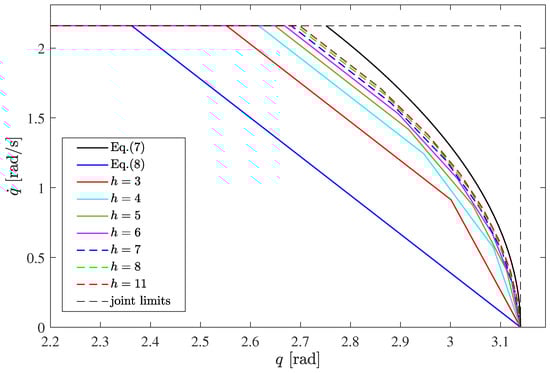
Figure 3.
Comparison of the viable polyhedrons for different values of h (portion of interest of the first quarter) in the case .
An analogous example is performed by using . The values of the normalized area of are shown in Table 2 and the resulting viable sets are depicted in Figure 4. The results lead to conclusions similar to the ones given by the previous example. However, it is clear that the magnitude of the phenomenon grows as the acceleration limits get smaller.
Table 2.
Inner area of for different values of h in case .
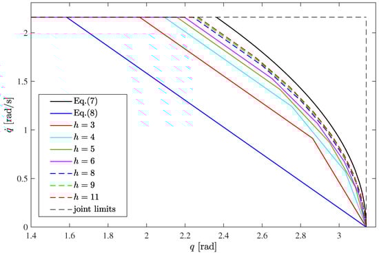
Figure 4.
Comparison of the viable polyhedrons for different values of h (portion of interest of the first quarter) in the case .
Of course the use of a larger value of h also gives some drawbacks. First, the computational complexity of Equation (23) rapidly grows with h as the number of variables and constraints is linear in h. As an example, the time needed to solve Equation (23) for and was in the order of 1 second and 15 s, respectively (the computation was performed in Matlab using a multi-start gradient-descent method on a standard laptop mounting a 2.5 GHz Intel Core i5-2520M processor).
Furthermore, the value of h determines the number of linear inequalities describing the polyhedron. In optimization-based control algorithms (such as linear MPC), this affects the computational complexity of the online optimal control problem, which is typically a critical issue in online methods, as mentioned in Section 1.
5. Experimental Results
Experimental were also performed on a six-degrees-of-freedom Universal Robot UR10 manipulator to prove the validity of the proposed approach. For the purposes of the paper, the joint position and velocity limits have been set to slightly conservative values with respect to the ones given in the datasheet. In particular, they are set as:
The acceleration limits have been set as . The experimental platform is shown in Figure 5. The objective of these experiments was the evaluation of the performance of an optimization-based control algorithm when different viability constraints are implemented. To this purpose, a simple MPC scheme was applied to a trajectory following problem. The MPC control scheme is in charge of following a position reference signal in the joint space. The model implemented in the MPC consists of a double integrator for each joint, as typical of robot kinematic control [15,30]. The input action is therefore represented by the joint accelerations, which then feed the low-level controller of the robot. Joint position, velocity, and acceleration limits can be implemented as linear constraints in the MPC (see [15] for details) and the online optimal control problem results to be a QP which minimizes the weighted sum of the tracking error and the control effort, as typical of linear MPC [31]. Notice that the choice of such a simple control scheme is due to the will of highlighting the behavior of a linear MPC controller in the case of different viability conditions. However, the proposed method could be straightforwardly applied to more complex MPC techniques such as [15,16,29].
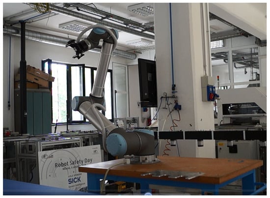
Figure 5.
Universal Robot UR10 used as experimental platform.
The MPC algorithm was implemented using a sampling period ms and by setting a predictive and a control horizon sampling periods. The robot trajectory is controlled by means of a ROS-based control architecture. Namely, a position controller runs in a ROS Kinetic Ubuntu 16.04. The controller communicates with the robot by means of a TCP connection. The controller takes the MPC position output as reference and receives the actual joint position. The controller output is the sum of a proportional action, with gain equal to seven, and a feedforward term equal to the MPC velocity output.
We considered a simple trajectory given by a straight line in the joint space, parameterized with respect to the normalized longitudinal length along the path, denoted with . The trajectory is therefore defined as:
where rad and rad are the initial and the final points of the trajectory, respectively, and is defined as a timing law with trapezoidal velocity profile, where represents the total time of the trajectory, as depicted in Figure 6.
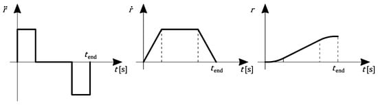
Figure 6.
Timing law with trapezoidal velocity profile.
The control problem the MPC controller has to solve at each cycle k therefore results:
where Q, , and are the joint position, velocity, and acceleration vectors, respectively, and the controller effort weighting factor was tuned empirically. Different implementations of the position limits will then be added to the problem in order to evaluate the different behaviors of the system.
As a first example, the total time of the trajectory was chosen as s and the behavior of the MPC controller was evaluated in three different scenarios:
- No position bounds are implemented.
- Box position constraints are implemented, which means that the following constraints are added to Equation (34):
- The linear viability condition in Equation (8) is applied, that is, Equation (35), and the following constraint are added to Equation (34):where the subscript i denotes the ith element of the vector.
The viability constraints are imposed throughout the whole control horizon for the sake of clarity and because the small increment in the computational time (due to the larger number of linear constraints) does not represent a significant issue in the presented experimental tests. However, in the case of linear MPC, imposing such constraints only on the last time instant of the horizon would be enough to ensure feasibility of the control problem and would not give significant differences in terms of control performance. The imposition of the constraint throughout the whole horizon permits to obtain a more reliable prediction of the future trajectory. This can be helpful especially in the case the prediction is utilized in linearized methods such as [15], as a non-reliable prediction might worsen the performance of the method.
Notice that the trajectory is devised in such a way that the desired motions of the first and the sixth joints exceed the maximal viable set, as shown in Figure 7a,b. The figures also show the phase plot of the position/velocity variables computed by the MPC in the three above-mentioned cases. In the case no position bounds are implemented (dashed green line), the joint position obviously does not satisfy the position limit. However, when box position constraints are implemented in the MPC (dash-dotted purple line), infeasibility of the control problem occurs and, since that time, the joint is forced to decelerate with the maximum admissible deceleration, but the position limit cannot be satisfied anyway. This highlights the importance of the viability property. In fact, the implementation of the linear constraints in Equation (8) does ensure the feasibility of the control problem and permits to satisfy the position bound (with a deformation of the original trajectory) (dashed red line). These behaviors are clarified also in Figure 8a,b, where the ideal and the measured joint positions for Joint 1 and Joint 6 are shown.
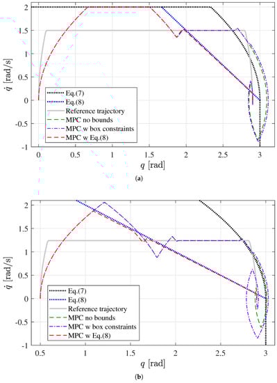
Figure 7.
State trajectory in the -plane for (a) Joint 1 and (b) Joint 3 for s: Reference trajectory (gray solid line); MPC without position bounds (green dashed line); MPC with box position bounds (purple dash-dot line); MPC with linear viability inequality (Equation (8)) (red dashed line); maximal viable set (black dotted line); and linear viability inequality ((Equation (8)) (blue dotted line).
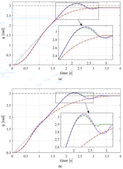
Figure 8.
Position of (a) Joint 1; and (b) Joint 3 for s: Reference trajectory (gray solid line). Output of MPC given as reference signal to the low-level controller: MPC without position bounds (green dotted line); MPC with box position bounds (purple dotted line); and MPC with linear viability inequality (Equation (8)) (red dotted line). Measured position: MPC without position bounds (green dashed line); MPC with box position bounds (purple dash-dot line); and MPC with linear viability inequality (Equation (8)) (red dashed line).
A second experiment is performed by choosing a total trajectory time s. In this case, the trajectory drives the first and the third joints in the region between Equations (7) and (8). The behavior of the MPC controller is evaluated in cases where three different viability constraints are implemented:
- The linear viability condition in Equation (8), that is, Equation (36) is added to Equation (34).
- The viable polyhedron obtained by solving Equation (23) with , that is, the following constraints are added to Equation (34):where the superscript i denotes the viable polyhedral of the ith joint.
- The viable polyhedron obtained by solving Equation (23) with , that is, the following constraints are added to Equation (34):
Figure 9a,b shows the state trajectory for the first joint in the three different cases. Notice that the position limit is respected and the control problem remains feasible for all cases. However, the reduction of the admissible region determined by Equation (8) gives rise to a significant modification of the original trajectory, although the desired states are always potentially realizable by the robot (as the trajectory does not exceed Equation (7)). An improvement is obtained when the polyhedron with is used.
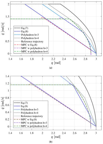
Figure 9.
State trajectory in the -plane for (a) Joint 1 and (b) Joint 3 for s: Reference trajectory (gray solid line); MPC with linear viability inequality (Equation (8)) (red dashed line); MPC implementing the viable polyhedron with (purple dash-dot line); and MPC implementing the viable polyhedron with (dashed green). Viable sets: Maximal (black dotted line); Linear viability inequality (Equation (8)) (blue dotted line); Polyhedron with (light blue dotted line); and Polyhedron with (gray dotted line).
Notice that the small velocity bumps visible in the figures are due to predictive nature of the controller. In fact, as the control scheme is based on the tracking of a position reference along the predictive horizon, the controller slightly increases the velocity when it realizes the viability constraint will be activated and a deformation of the task will arise (as the state will be forced to follow the constraint). By giving a small acceleration before the activation of the constraint, the controller minimizes the future deviation with respect to the given position reference.
Finally, the use of permits to obtain a viable polyhedron that is large enough to enclose the whole desired trajectory. These behaviors are clarified also in Figure 10a,b, where the ideal and the measured joint positions for Joint 1 and Joint 6 are shown.
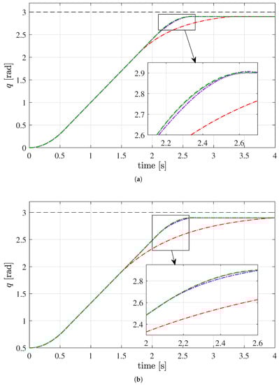
Figure 10.
Position of (a) Joint 1 and (b) Joint 3 for s. Reference trajectory (gray solid line). Output of MPC given as reference signal to the low-level controller: MPC with linear viability inequality (Equation (8)) (red dotted line); MPC implementing the viable polyhedron with (purple dotted line); and MPC implementing the viable polyhedron with (green dotted line). Measured position: MPC with linear viability inequality (Equation (8)) (red dashed line); MPC implementing the viable polyhedron with (purple dash-dot line); and MPC implementing the viable polyhedron with (green dashed line).
6. Conclusions
In this paper, we have proposed a method to compute the maximal viable polyhedron for a robot manipulator with bounded joint positions, velocities, and accelerations. In the proposed approach, each joint is considered separately and two optimization problems are devised: one for the upper bounds and one for the lower ones. Given its number of sides, the resulting polyhedron maximizes the area of the admissible position/velocity region. Moreover, the set is proven to be viable and convex. In this way, it can be easily implemented as linear constraints in optimization-based control methods, such as linear MPC. Numerical results demonstrate that the percentage of area covered by the polyhedrons increases as the number of sides grows. This allows the controller to exploit a larger admissible state region and, thus, gives it a broader margin of maneuver in the case the desired motion drives the robot in proximity of the viability boundary. In this case, a better task following can be achieved, as demonstrated by means of experimental results on a six-degrees-of-freedom manipulator.
Author Contributions
M.F. devised the method and wrote the paper; M.B. and N.P. conceived and performed the experiments; and A.V. supervised the whole research work.
Funding
The research leading to these results was partially funded by the European Union H2020-CS2-738039-Eureca: Enhanced Human Robot cooperation in Cabin Assembly tasks.
Conflicts of Interest
The authors declare no conflict of interest.
References
- Verscheure, D.; Demeulenaere, B.; Swevers, J.; Schutter, J.D.; Diehl, M. Time-Optimal Path Tracking for Robots: A Convex Optimization Approach. IEEE Trans. Autom. Control 2009, 54, 2318–2327. [Google Scholar] [CrossRef]
- Riazi, S.; Wigström, O.; Bengtsson, K.; Lennartson, B. Energy and Peak Power Optimization of Time-Bounded Robot Trajectories. IEEE Trans. Autom. Sci. Eng. 2017, 14, 646–657. [Google Scholar] [CrossRef]
- Kazerounian, K.; Wang, Z. Global versus local optimization in redundancy resolution of robotic manipulators. Int. J. Robot. Res. 1988, 7, 3–12. [Google Scholar] [CrossRef]
- Faroni, M.; Beschi, M.; Visioli, A.; Molinari Tosatti, L. A global approach to manipulability optimisation for a dual-arm manipulator. In Proceedings of the IEEE International Conference on Emerging Technologies and Factory Automation, Berlin, Germany, 6–9 September 2016; pp. 1–6. [Google Scholar]
- Lee, J.; Chang, P.H. Redundancy resolution for dual-arm robots inspired by human asymmetric bimanual action: Formulation and experiments. In Proceedings of the IEEE International Conference on Robotics and Automation, Seattle, WA, USA, 26–30 May 2015; pp. 6058–6065. [Google Scholar]
- Liegeois, A. Automatic Supervisory Control of the Configuration and Behavior of Multibody Mechanisms. IEEE Trans. Syst. Man Cybern. 1977, 7, 868–871. [Google Scholar]
- Cheng, F.T.; Chen, T.H.; Sun, Y.Y. Resolving manipulator redundancy under inequality constraints. IEEE Trans. Robot. Autom. 1994, 10, 65–71. [Google Scholar] [CrossRef]
- Kanoun, O.; Lamiraux, F.; Wieber, P.B. Kinematic control of redundant manipulators: Generalizing the task priority framework to inequality tasks. IEEE Trans. Robot. 2011, 27, 785–792. [Google Scholar] [CrossRef]
- Escande, A.; Mansard, N.; Wieber, P.B. Hierarchical quadratic programming: Fast online humanoid-robot motion generation. Int. J. Robot. Res. 2014, 33, 1006–1028. [Google Scholar] [CrossRef]
- Liu, M.; Tan, Y.; Padois, V. Generalized hierarchical control. Auton. Robots 2016, 40, 17–31. [Google Scholar] [CrossRef]
- Rocchi, A.; Hoffman, E.M.; Caldwell, D.G.; Tsagarakis, N.G. Opensot: A whole-body control library for the compliant humanoid robot Coman. In Proceedings of the IEEE International Conference on Robotics and Automation, Seattle, WA, USA, 26–30 May 2015; pp. 6248–6253. [Google Scholar]
- Siciliano, B.; Slotine, J.J.E. A general framework for managing multiple tasks in highly redundant robotic systems. In Proceedings of the International Conference on Advanced Robotics, Pisa, Italy, 19–22 June 1991; pp. 1211–1216. [Google Scholar]
- Flacco, F.; De Luca, A. Discrete-time redundancy resolution at the velocity level with acceleration/torque optimization properties. Robot. Auton. Syst. 2015, 70, 191–201. [Google Scholar] [CrossRef]
- Flacco, F.; De Luca, A.; Khatib, O. Control of Redundant Robots Under Hard Joint Constraints: Saturation in the Null Space. IEEE Trans. Robot. 2015, 31, 637–654. [Google Scholar] [CrossRef]
- Faroni, M.; Beschi, M.; Visioli, A.; Molinari Tosatti, L. A Predictive Approach to Redundancy Resolution for Robot Manipulators. In Proceedings of the IFAC World Congress, Toulouse, France, 9–14 July 2017; pp. 8975–8980. [Google Scholar]
- Faroni, M.; Beschi, M.; Visioli, A. Predictive Inverse Kinematics for Redundant Manipulators: Evaluation in Re-Planning Scenarios. In Proceedings of the IFAC Symposium on Robot Control, Budapest, Hungary, 27–30 August 2018. [Google Scholar]
- Buizza Avanzini, G.; Zanchettin, A.M.; Rocco, P. Reactive Constrained Model Predictive Control for Redundant Mobile Manipulators. In Intelligent Autonomous Systems 13, Advances in Intelligent Systems and Computing; Springer: Berlin/Heidelberg, Germany, 2016; pp. 1301–1314. [Google Scholar]
- Ghazaei Ardakani, M.M.; Olofsson, N.; Robertsson, A.; Johansson, R. Real-Time Trajectory Generation using Model Predictive Control. In Proceedings of the IEEE International Conference on Automation Science and Engineering, Gothenburg, Sweden, 24–28 August 2015; pp. 942–948. [Google Scholar]
- Ferrara, A.; Incremona, G.P.; Magni, L. A robust MPC/ISM hierarchical multi-loop control scheme for robot manipulators. In Proceedings of the Annual Conference on Decision and Control, Florence, Italy, 10–13 December 2013; pp. 3560–3565. [Google Scholar]
- Blanchini, F. Set invariance in control. Automatica 1999, 35, 1747–1767. [Google Scholar] [CrossRef]
- Saab, L.; Ramos, O.E.; Keith, F.; Mansard, N.; Soueres, P.; Fourquet, J.Y. Dynamic whole-body motion generation under rigid contacts and other unilateral constraints. IEEE Trans. Robot. 2013, 29, 346–362. [Google Scholar] [CrossRef]
- Park, K.C.; Chang, P.H.; Kim, S.H. The enhanced compact QP method for redundant manipulators using practical inequality constraints. In Proceedings of the IEEE International Conference on Robotics and Automation, Leuven, Belgium, 20 May 1998; pp. 107–114. [Google Scholar]
- Kanehiro, F.; Morisawa, M.; Suleiman, W.; Kaneko, K.; Yoshida, E. Integrating geometric constraints into reactive leg motion generation. In Proceedings of the IEEE/RSJ International Conference on Intelligent Robots and Systems, Taipei, Taiwan, 18–22 October 2010; pp. 4069–4076. [Google Scholar]
- Wensing, P.M.; Orin, D.E. Generation of dynamic humanoid behaviors through task-space control with conic optimization. In Proceedings of the IEEE International Conference on Robotics and Automation, Karlsruhe, Germany, 6–10 May 2013; pp. 3103–3109. [Google Scholar]
- Guarino Lo Bianco, C.; Gerelli, O. Online trajectory scaling for manipulators subject to high-order kinematic and dynamic constraints. IEEE Trans. Robot. 2011, 27, 1144–1152. [Google Scholar] [CrossRef]
- Scheint, M.; Wolff, J.; Buss, M. Invariance control in robotic applications: Trajectory supervision and haptic rendering. In Proceedings of the IEEE American Control Conference, Seattle, WA, USA, 11–13 June 2008; pp. 1436–1442. [Google Scholar]
- Zanchettin, A.M.; Rocco, P. Motion planning for robotic manipulators using robust constrained control. Control Eng. Pract. 2017, 59, 127–136. [Google Scholar] [CrossRef]
- Del Prete, A. Joint Position and Velocity Bounds in Discrete-Time Acceleration/Torque Control of Robot Manipulators. IEEE Robot. Autom. Lett. 2018, 3, 281–288. [Google Scholar] [CrossRef]
- Faroni, M.; Beschi, M.; Pedrocchi, N.; Visioli, A. Predictive Inverse Kinematics for Redundant Manipulators with Task Scaling and Kinematic Constraints. IEEE Trans. Robot 2018. submitted. [Google Scholar]
- Gerelli, O.; Guarino Lo Bianco, C. Nonlinear variable structure filter for the online trajectory scaling. IEEE Trans. Ind. Electron. 2009, 56, 3921–3930. [Google Scholar] [CrossRef]
- Wang, L. Model Predictive Control System Design and Implementation Using MATLAB®; Springer Science & Business Media: Berlin/Heidelberg, Germany, 2009. [Google Scholar]
© 2018 by the authors. Licensee MDPI, Basel, Switzerland. This article is an open access article distributed under the terms and conditions of the Creative Commons Attribution (CC BY) license (http://creativecommons.org/licenses/by/4.0/).