


Semantic Segmentation and Roof Reconstruction of Urban Buildings Based on LiDAR Point Clouds

1
School of Civil Engineering and Geomatics, Shandong University of Technology, Zibo 255000, China
2
Hubei Luojia Laboratory, Wuhan 430079, China
*
Author to whom correspondence should be addressed.
ISPRS Int. J. Geo-Inf. 2024, 13(1), 19; https://doi.org/10.3390/ijgi13010019
Submission received: 14 November 2023
/
Revised: 29 December 2023
/
Accepted: 4 January 2024
/
Published: 5 January 2024
(This article belongs to the Special Issue Unlocking the Power of Geospatial Data: Semantic Information Extraction, Ontology Engineering, and Deep Learning for Knowledge Discovery)
Abstract
:In urban point cloud scenarios, due to the diversity of different feature types, it becomes a primary challenge to effectively obtain point clouds of building categories from urban point clouds. Therefore, this paper proposes the Enhanced Local Feature Aggregation Semantic Segmentation Network (ELFA-RandLA-Net) based on RandLA-Net, which enables ELFA-RandLA-Net to perceive local details more efficiently by learning geometric and semantic features of urban feature point clouds to achieve end-to-end building category point cloud acquisition. Then, after extracting a single building using clustering, this paper utilizes the RANSAC algorithm to segment the single building point cloud into planes and automatically identifies the roof point cloud planes according to the point cloud cloth simulation filtering principle. Finally, to solve the problem of building roof reconstruction failure due to the lack of roof vertical plane data, we introduce the roof vertical plane inference method to ensure the accuracy of roof topology reconstruction. The experiments on semantic segmentation and building reconstruction of Dublin data show that the IoU value of semantic segmentation of buildings for the ELFA-RandLA-Net network is improved by 9.11% compared to RandLA-Net. Meanwhile, the proposed building reconstruction method outperforms the classical PolyFit method.
1. Introduction
Three-dimensional city modeling [1,2,3] is widely used in urban planning, smart city development, navigation, virtual reality, and other fields. Since LiDAR can directly acquire dense 3D point clouds of buildings, LiDAR data have become a widely used data source in 3D building model reconstruction.
Current building reconstruction methods are divided into two main categories: model-driven building reconstruction methods [4,5,6,7,8] and data-driven building reconstruction methods [9,10,11,12,13]. Model-driven methods generate a 3D model of a building by combining building primitives through predefined building primitives after selecting the optimal primitives. Although this method is capable of generating 3D models with correct topology, it is difficult to define a set of primitives that can effectively represent various building shapes due to the variety of building structures in a building. Instead of matching predefined building primitives, data-driven methods infer the structure of buildings from point cloud data, which provides better flexibility than model-driven methods and is more suitable for reconstructing models of complex buildings in urban scenes. Although some data-driven methods [14,15,16,17] have been developed to automatically generate high-quality building models using airborne LiDAR point cloud data, data-driven methods still face the following problems when reconstructing buildings from LiDAR point clouds in urban scenes:
Building Instance Segmentation. The complex shape and many types of features in urban scenes, the significant amount of point cloud data and the sparse distribution make the recognition and separation of single buildings a great challenge.
Automatic Roof Plane Recognition. Building plane point cloud segmentation and recognition of roof plane primitives are the basis of building roof model reconstruction. The recognition of the roof plane, although it can be judged by the combined direction and height of the normal vector of the plane, requires appropriate thresholds to be set for point cloud buildings of different heights.
The roof point cloud data is incomplete. Due to the restricted scanning direction of the airborne scanner, some important building structures, such as vertical walls on the roof of a building, usually cannot be captured completely in the airborne LiDAR point cloud.
In this paper, we solve the above problems by the following strategies. First, we use the semantic segmentation method to segment the building point cloud from the urban LiDAR point cloud and then utilize the clustering method to extract single buildings from the building point cloud to solve the problem of building instance segmentation. Secondly, the principle of cloth simulation filtering is utilized to automatically identify the roof point cloud plane. Finally, this paper proposes a building topology reconstruction method based on roof vertical plane inference to solve the problem of topology reconstruction failure due to defective roof point cloud data quality. The main contributions of this work include:
- Propose a semantic segmentation network based on enhanced local feature aggregation. The network enhances the point-by-point local features from both structural information and semantic information to realize effective semantic segmentation of building point clouds.
- Propose a roof surface point cloud automatic identification method to extract the roof point cloud plane.
- Propose a building topology reconstruction method based on roof vertical plane inference to realize the topology reconstruction of buildings.
2. Related Work
In this section, we focus on methods related to our approach.
Building point cloud semantic segmentation. Currently, some deep learning-based point cloud semantic segmentation efforts [18,19,20,21,22] have achieved satisfactory results, but due to their higher model complexity, they usually require a large number of computational resources, which restricts the application of these methods in urban point cloud scenarios. RandLA-Net [23] is an efficient and lightweight semantic segmentation network, which is designed to capture the local geometric information of the point cloud by employing a random sampling algorithm to downsample each layer of the encoder and introduces an efficient local feature aggregation unit for capturing the local geometric information of the point cloud. In order to efficiently handle large-scale point clouds, this paper chooses to improve the RandLA-Net network and further improve the point-by-point classification accuracy of buildings by enhancing the local features at each point.
Segmentation of building planes. Random Sample Consistency (RANSAC) [24] and region growing algorithms [25,26,27] are currently well-established methods for segmentation of planar primitives. Because the RANSAC method exhibits robustness to noise and outliers in plane segmentation, we chose it to extract building plane primitives. In addition, RANSAC targets spatial consistency and segments the planes in the point cloud sequentially through an iterative approach, which tends to lead to the problem of competing segmentation planes and ultimately obtains suboptimal segmentation results [28]. To improve the method plane segmentation problem, we further refine the extracted plane primitives.
Building Regularized Contour Extraction. Some methods [29,30,31,32] extract a collection of building contour straight lines through the Alpha Shape [33] algorithm and adjust the orientation of the contour straight lines by calculating the main direction of the building so that the building contour conforms to the structural regularity of the building. Some methods [34,35] form building boundary polygons by detecting building corner points and then connecting them. In this paper, regularized roof plane polygons are extracted using the method described in [31].
Model-driven building reconstruction methods. Model-driven approaches [4,5,6,7,8] reconstruct building models by combining predefined parameterized building primitives. Costantino et al. [4], for modeling complex structures, pointed out that by introducing an interactive editing phase, the model-driven approach can improve the reconstruction accuracy when reconstructing 3D models and the effects of different building footprint segmentation methods on the accuracy and precision of model-driven modeling were also discussed in depth. Xiong et al. [6] found that errors in topological maps will seriously affect the final model-driven modeling results, so a strategy based on a dictionary of graph editing operations is proposed to automatically identify and correct errors in the input graph. Xiong et al. [7] improved the flexibility of model reconstruction by defining basic building primitives via loose nodes, loose edges, and minimum cycles in the roof topology graph. Huang et al. [8] proposed a method for model-driven reconstruction of pylons for tilted UAV images. Li et al. [5] performed primitive segmentation via a two-step RANSAC strategy and overall primitive fitting to reconstruct topologically consistent 3D building models. However, this class of methods is still limited by predefined building primitives.
Data-driven building reconstruction methods. Some building topology reconstruction methods [9,10,12,13,36] focus on constructing closed polygons of roofs by establishing topological relationships between roof planes [37] and determining the boundaries between the planes where topological information exists. For example, Chen et al. [9] utilized a Voronoi subgraph-based to recover topological relationships between roof plane primitives for a watertight and compact reconstruction of the building model. Li et al. [10] introduced a new elevation-preferred resource formulation to physically balance higher roofs and other roof planes, constrain the selection of building model planes, and ensure topological correctness of the reconstructed model. Sampath et al. [12] represented the topological relationships between roof planes using an adjacency matrix, which is used to determine the ridges, edges and vertices of the building model for the final reconstruction. Wang et al. [13] proposed a point-based method for 3D building roof reconstruction. The core objective of this method is to generate points that are used to represent and connect the roof layers of the building roof. These points are named layer connectors. Layer connectors serve two purposes, i.e., to represent the roof layers horizontally and to connect the different roof layers vertically. Recently, some studies [11,38,39,40] have used deep learning methods to reconstruct building roof models. For example, Li et al. [11] transformed the problem of modeling building roofs into a vertex detection and edge prediction problem for the reconstruction of building roofs. In addition, some studies [14,15,16,17] used a spatial partitioning approach for building reconstruction. The spatial partitioning-based building reconstruction method divides the 3D space into polyhedral space by extending the plane primitives and generates the polyhedral model by optimally selecting the optimal subset of candidate planes. For example, Nan et al. [16] generated a sizable set of candidate planes by intersecting plane primitives and then selected the optimal subset of candidate planes by optimization. Liu et al. [15] solved the problem of plane primitive loss in segmentation by segmenting plane primitives from incomplete point clouds, detecting feature lines in point clouds and images, and recovering missing planes with the relationship between linear and plane primitives to avoid triggering topological errors in the reconstruction of complex building models. Yang et al. [17] proposed a confidence strategy incorporating the graph structure to generate candidate face sets through the neighbor relationship between plane primitives. In this paper, we use a building topology reconstruction method for building reconstruction, with special consideration for the problem of roof topology reconstruction failure due to missing data. To this end, we will reconstruct the building model by replacing the data quality-deficient roof vertical plane with the inferred roof vertical plane.
Reconstruction of building models from lidar point clouds. Reconstruction of building models from lidar point clouds methods [14,41,42,43], in general, involves the structured reconstruction of the point clouds of each building in order to achieve a complete reconstruction of the overall building. The differences between the different methods mainly lie in the way the point cloud of a single building is acquired and the specific reconstruction method. For example, Zhang et al. [43] proposed a rectified linear unit’s neural network named ReLu-NN to classify the point clouds and used a 2.5D contouring method [44] to reconstruct the building model. Sahebdivani et al. [42] used PointNet [45] deep learning network, and the model reconstructed by Poisson [46] was subsequently simplified using vertex clustering and edge collapse with quadratic error, and finally, a lightweight building model was obtained. Huang et al. [14] utilized the existing footprint polygon data to achieve the extraction of single building point clouds, and also proposed a method to infer vertical walls directly from the data and achieved the reconstruction of regional buildings by using extended assumptions and a selection-based polygon surface reconstruction framework, but the monolithic footprints of the buildings were limited by the polygonal data. In this paper, we propose a semantic segmentation network with an encoder–decoder structure for acquiring point clouds of semantic categories of buildings and accomplishing the reconstruction of roof models of buildings by recovering the roof topology. The difference with previous methods is that the encoder part of the network in this paper uses a random sampling algorithm to downsample the point cloud, while the network structure of [43] uses fully connected linear cells without downsampling the point cloud, and the PointNet network of [42] uses a coder–decoder structure but uses a farthest-points sampling algorithm for downsampling. Compared with these two methods, this paper has higher efficiency in processing large-scale point clouds. In addition, the methods of [42,43] represent the building model by simplifying the mesh. The mesh model is not suitable for model storage and may lead to sharp boundaries of the building contours.
3. Methodology
3.1. Overview
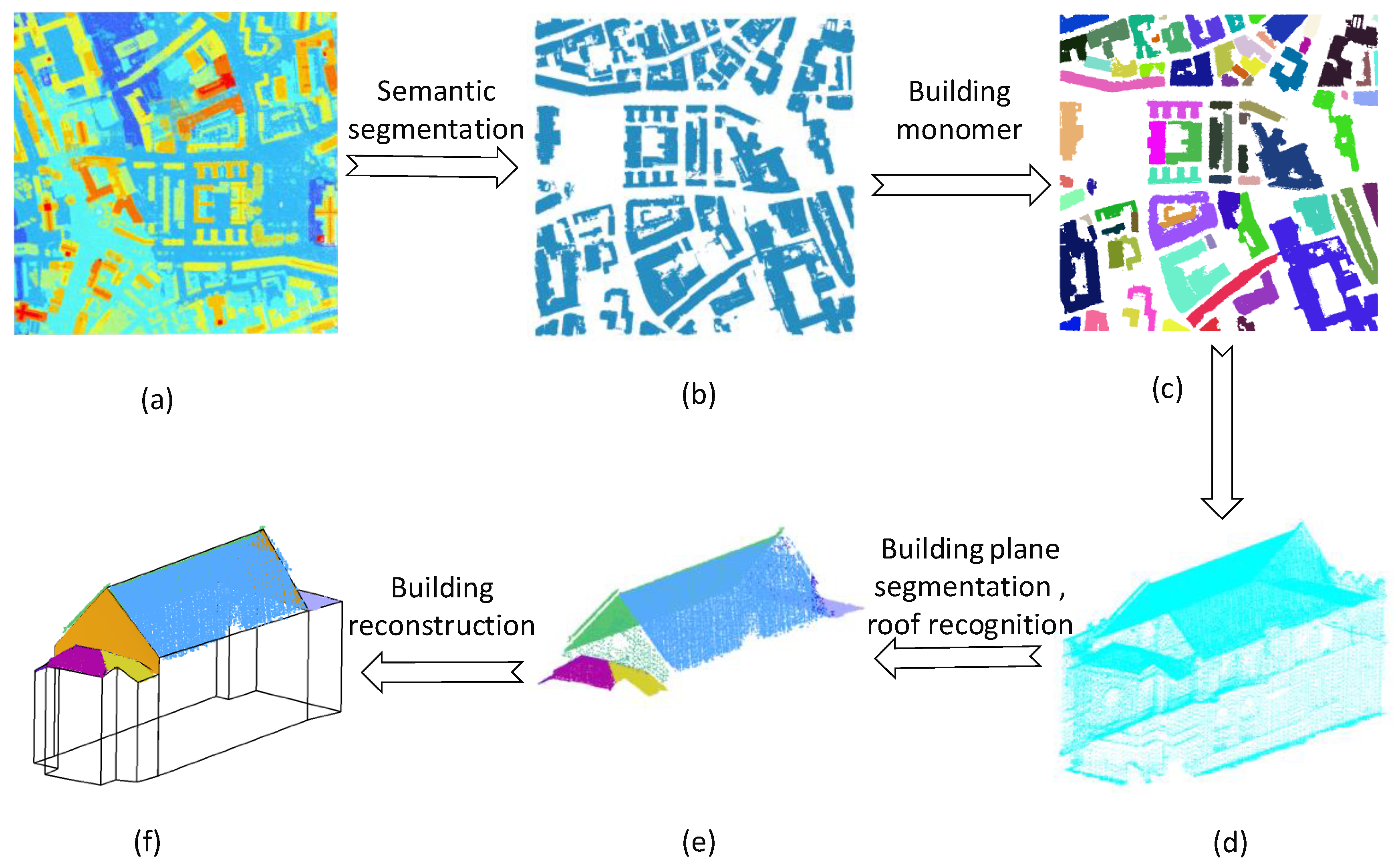
In this paper, original LiDAR point clouds of urban scenes were taken as input and structured models of buildings were output. First, the building point cloud was recognized and extracted from the original LiDAR point cloud by semantic segmentation, and the single building was extracted from the building point cloud using clustering. Next, the single building plane was segmented, and the roof plane was automatically recognized. Finally, the topological reconstruction of the roof was performed by replacing the corresponding vertical plane with the inferred vertical plane of the roof, and the outer contour of the roof was extended to the ground to complete the reconstruction of the 3D building model. The reconstruction process is shown in Figure 1.
3.2. Semantic Segmentation of Building Point Clouds Based on Enhanced Local Feature Aggregation
In this paper, we design a semantic segmentation network based on Enhanced Local Feature Aggregation, hereinafter referred to as ELFA-RandLA-Net. The network structure is shown in Figure 2. The proposed network uses an encoder–decoder structure. The encoder progressively extracts high-level, abstract features of the point cloud, and the decoder propagates these features to each point for point-by-point prediction. Both the encoder and decoder are four-layer structures. Each layer of the encoder includes a local feature aggregation module and point cloud downsampling, and each layer of the decoder includes an inverse convolution module and point cloud upsampling. In the encoding stage, the proposed enhanced local feature aggregation module extracts point-by-point local features, randomly samples for point cloud downsampling, and obtains global features of the point cloud through layer-by-layer feature extraction and downsampling. In the decoding stage, the inverse convolution [23] maps the global features to the low-dimensional feature space, and linear interpolation [23] recovers the number of point clouds. Finally, the network outputs the probabilistic predicted value of each point.
The Enhanced Local Feature Aggregation (ELFA) module is the key module of the proposed network, and the basic idea is to characterize each point using enhanced local features. ELFA consists of a local feature coding and hybrid pooling unit, which enhances the local features by using geometric coding and semantic coding and aggregates the local features of each point by maximal pooling and attention pooling. The inputs to the enhanced local feature aggregation module are the 3D coordinates of each point and the corresponding features. First, the module collects the nearest neighboring points of each location and constructs the neighborhood by KNN algorithm. Next, the positional coding submodule is used to extract the geometric information of the neighborhood, while the semantic coding submodule is used to extract the semantic information within the neighborhood, and the geometric features are concatenated with the semantic features to obtain the enhanced local features. Finally, the hybrid pooling submodule aggregates the maximum and attention features within the neighborhood and outputs the summed neighborhood features to accurately aggregate the neighborhood features. The details of ELFA module are shown in Figure 3, and its principle is as follows:
Given an input point set and its corresponding feature . For simplicity, only one spatial location is subjected to local feature aggregation in this section, while the enhanced local feature aggregation method can be applied to local feature extraction for the entire point set. denotes a spatial location in the point set (3D coordinates, ).
- (1)
- Local feature coding.
Neighbor point query. The K Nearest Neighbors (KNN) algorithm [47] is a neighbor point search method that computes the nearest points around a point in Euclidean space and is suitable for constructing point-by-point neighborhoods. The KNN algorithm collects the nearest neighbors of each point in a point cloud to form a radius neighborhood. In the concrete implementation, for each location , it is used as a query point to find the nearest neighbors in the point set , these nearest neighbors are called the neighbor points of , and their set is denoted as .
Position Encoding (PE). For the neighbor point at each location , the input features of the neighbor point are explicitly encoded using geometric information such as the spatial location of the neighbor point, the spatial location of the query point, the relative position of the neighbor point to the query point, and the distance between them:
where is the spatial location of the neighboring points, is the relative position of the neighboring points to the query point, and is the computed Euclidean distance. ⨁ is the vector concatenation.
Semantic Encoding (SE). For the neighbor point at each location , the input features of the neighbor point are implicitly encoded using semantic information such as the features of the neighbor point, the features of the query point, and the relative features of the neighbor point and the query point:
where is the input feature corresponding to position , is the feature corresponding to neighbor point , and is the relative feature (edge feature).
Feature Enhancement. The multilayer perceptron (MLP) [45], consists of multiple 1 × 1 convolutions that can be used to extract abstract features of a point cloud and to implement dimensional transformations of the feature vectors. By aligning the spatial location and semantically encoded vector dimensions in a concatenation via MLP, the augmented neighbor point feature representation for each location can be obtained:
Finally, the set of enhanced features corresponding to the set of neighboring points at any position is .
- (2)
- Mixed Pooling.
Max pooling can effectively summarize the neighborhood information, and attention pooling can distinguish the neighborhood features and retain more details. Therefore, the combination of both can more accurately represent the local features of a point.
Max pooling is the selection of the most salient feature about a given location to summarize the local context at that location, which is formally defined as follows:
Attention pooling computes attention weights to weight local features by the score function , and applies the attention weights to neighboring point features and sums them to achieve weighted aggregation of local features. It is defined as:
where is the learnable parameter matrix, is composed of the shared MLP and the normalization function [45], · denotes the corresponding element multiplication (Hadamard product), and the dimensions of the attention weight vector and the input need to be matched.
The features of the max pooling feature and the attention pooling feature in concatenation as the features after aggregation at any position :
where is the output feature after mixed pooling at location .
In summary, given a location , ELFA module can effectively aggregate the local geometric and semantic information of the spatial location and finally generate a feature vector after neighbor point query, location and semantic encoding of neighbor point feature enhancement and mixed pooling of local feature aggregation.
3.3. Building Point Cloud Plane Segmentation and Roof Plane Identification
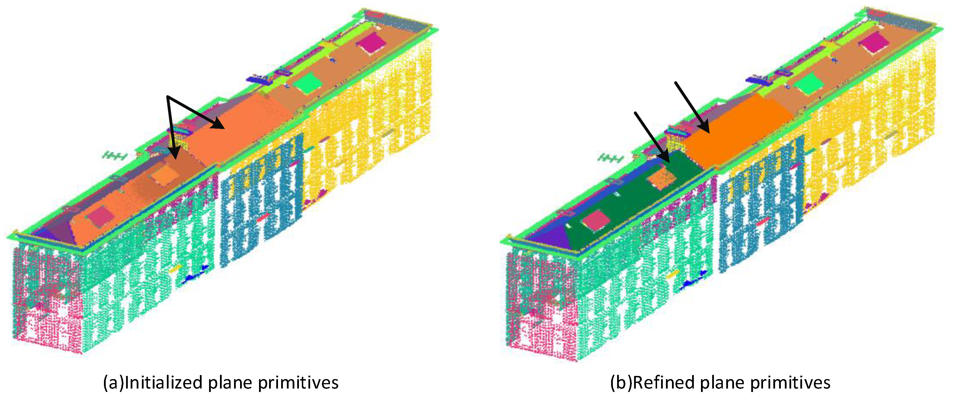
For different roof planes with a small height difference and a gentle transition (e.g., the roof planes indicated by the arrows in Figure 4a), the RANSAC plane segmentation may suffer from the problem of different roof planes being incorrectly classified into the same plane since the height difference between the two roof planes is smaller than the point-to-plane distance threshold preset by the RANSAC algorithm. Therefore, we utilize the Density-Based Spatial Clustering of Applications with Noise (DBSCAN) [48] algorithm to resegment the RANSAC misclassified planes. In addition, in order to automatically identify the roof planes, we use the Cloth Simulation Filter (CSF) [49] principle to simulate the shape of the roof and the building planes to which the shape of the roof is less than a certain threshold are considered roof planes.
The building point cloud plane segmentation and roof plane recognition process, as shown in Figure 4, has the following steps:
(1) Building plane segmentation. In this paper, the RANSAC [24] algorithm is used to detect the plane of the building point cloud as the initial plane primitive.
(2) Initial plane primitive’s refinement. The DBSCAN algorithm is a density clustering algorithm that divides the point cloud into different clusters by calculating the density around each point. Therefore, this paper uses the DBSCAN algorithm to optimize the initial plane primitives that contain multiple initial plane primitives of different point cloud planes of the building are resegmented. The RANSAC-segmented planes may contain some small plane primitives that are not meaningful for the reconstruction of the building, and in this paper, we will filter out the small plane primitives that have less point support.
(3) Automatic recognition of roof plane point cloud. Point cloud Cloth Simulation Filter (CSF) [49] is a method that uses a cloth model to simulate the surface of inverted terrain (terrain is turned upside down) to extract ground point clouds. In this paper, we use the principle of extracting ground point cloud by the CSF method and we extract the building roof plane point cloud by inverting the building point cloud and simulating the roof shape by using the cloth model.
CSF is a method for extracting ground point clouds by using a cloth model to simulate the surface of inverted terrain. The CSF method of extracting ground point clouds works by inverting the building point cloud (i.e., reversing the orientation of the building point cloud) and simulating the shape of the ground using a cloth model to extract the building ground point cloud. Without inverting the building point cloud, the CSF method can simulate the shape of the building roof. After obtaining the roof shape using the CSF method, the distance between the segmented building planes and the roof shape can be calculated, and the plane whose distance is less than a certain threshold can be selected as the roof plane. This process realizes the automatic identification and extraction of the roof plane.
3.4. Structured Reconstruction of Buildings Based on Roof Vertical Plane Inference
Due to the quality of the point cloud data of the vertical plane of the roof, the extracted vertical plane polygons are usually difficult to completely express the basic structure of the vertical plane of the roof. Incomplete roof vertical plane polygons will affect the judgment of roof plane adjacencies as well as the correction of building corner points. Therefore, this paper proposes a building topology reconstruction method based on vertical plane inference. The building reconstruction process of this paper’s method, shown in Figure 5, consists of five steps: (1) Determining the initial boundary vertices of the roof plane using the method in [31]; (2) inference of vertical planes in the roof; (3) judgment of adjacencies between the roof plane polygons, and construction of the roof topology map; (4) roof modeling topology reconstruction; (5) stretching the outer contour of the roof model to the ground to reconstruct the 3D model of the building.
3.4.1. Roof Vertical Plane Inference
The vertical plane in the roof of a building refers to the roof plane whose normal vector is approximately perpendicular to the principal axis direction . The point cloud data of the vertical plane of a building’s roof usually have missing or defective quality, as shown in the plane pointed by the red line in Figure 6a. It makes the polygon of the vertical plane of the roof unable to accurately represent the basic structure of the building, resulting in the topological error of the roof plane, which affects the reconstruction of the building. Therefore, in this paper, the original vertical plane is replaced by the fitted vertical plane to ensure the accuracy of the topological reconstruction of the building.
The basic idea of roof vertical plane fitting is based on a structural feature, namely, a large height difference between the pairs of roof planes connected by the roof vertical plane and the adjacency of the 2D projection planes of the connected planes. Firstly, the pairs of planes used to fit the vertical plane are determined, and then the vertical planes are fitted by using the adjacency edges of the pairs of planes. The methods are shown in Figure 6b–d. The specific methods are as follows:
(1) Determine the paired planes used to fit the vertical plane. If the distance between the paired roof planes projected onto the XOY plane is less than a set distance threshold and the height difference between the roof planes is less than a set height threshold, then it is determined that there exists a vertical plane for the paired planes.
(2) Fitting the roof vertical plane. First, determine the adjacent straight lines and between the paired neighboring planes, calculate the coordinates of the midpoints of the straight lines and , and , and use Equation (9) to calculate the unit direction vector of the straight line . Then, the 2D coordinates of the endpoints of the adjacent lines and are projected onto the line using Equations (10) and (11), and the elevation values of the projected endpoints are kept the same as those before projection, to obtain the projection points , which are the boundary vertices of the vertical plane.
where denote the coordinate vectors of the corresponding points, and and denote the coordinate vectors of the midpoints of the lines and , respectively; denotes the distance, is the normalized unit-direction vector, and denotes the direction of the projection; is the distance between the vector and the vector after dot-multiplication operation, which represents the distance from the point to in the direction of vector ; is the coordinate after moving a certain distance along the direction of with as the starting point, and denotes the relative position to m_ad in the projected direction. the position of in the projection direction.
3.4.2. Roof Plane Topology Map Construction
A roof topology graph is a representation consisting of roof planes (as nodes of the graph) and adjacencies between the planes (as edges of the graph). Each node represents a roof plane, and an edge represents an adjacency between two roof planes. When there is an adjacency between two roof planes, the corresponding nodes are connected to each other by edges.
The key to constructing a roof topology is to determine the adjacency between roof planes, which is determined by determining whether the expanded polygons of the roof planes intersect. The method of determining the adjacency between planes is shown in Figure 7 as follows:
(1) Polygon outward expansion. Since there is usually an error between the regularized boundary and the real roof plane boundary (usually shrinking to the inside of the roof plane), it is necessary to externally expand the boundary of the polygon. The outward expansion process will take the midpoint of the edge to be expanded as the starting point and expand a certain distance along the direction of each of the two endpoints, and the size of the distance is usually three times the average point cloud spacing, as shown in Figure 7a.
(2) Polygon intersection relationship judgment. By judging whether the outward expanding polygons are intersecting, the potential adjacency relationship between the planes is initially determined.
(3) Overlap check. The intersection in Figure 7b can be determined as the adjacency relationship between two planes, but there may be cases where the planes intersect and are not actually adjacent, as shown in Figure 7c. For this reason, it is necessary to calculate the ratio of the length of the intersecting straight line to the length of the shorter of the neighboring edges, to determine the degree of overlap of the intersecting parts of the polygon, and ultimately to determine the adjacency of the pairs of planes.
3.4.3. Roof Polygon Reconstruction
Roof corners can be divided into two categories: roof corners whose inner points are inside the roof contour lines and inner points that are intersections with at least three roof planes. The inner points can be determined by intersecting the planes corresponding to the smallest link points in the topological map. The outer points of a roof are roof vertices other than the inner points, which consist of two or fewer roof planes.
A roof polygon is a polygon constructed by using the coordinates of the building corner points to correct the vertex coordinates of the roof plane polygons and merging the corrected roof plane polygons. This section describes the building corner point search method and calculation method in the topological map, as well as the roof polygon method.
(1) Roof inner points detection and computation. The minimum ring base of the roof topology graph can be obtained by the Dijkstra algorithm [50], and the intersection point of the minimum ring base node corresponding to the roof plane is the inner points. In most cases, it is often difficult to find an exact solution for the intersection of roof planes, so it is necessary to solve the intersection using the least squares method of the plane intersection equation and the formulas for solving the intersection by the three plane least squares methods are (12), (13), and (14). The outer points of the roof are shown as yellow points in Figure 8a.
where , and, are the three plane equation coefficients, respectively.
(2) Roof outer points detection and computation. The outer points of a roof can be categorized into two types: one is the endpoints located on the intersecting lines of the roof plane and the other is the intersecting points located on the straight lines of the individual roof boundaries. They correspond to edges and loose nodes in the topological graph, respectively. As shown in Figure 8a, D, E, F, G, K, O, and P are located on roof plane intersection lines, and they are the endpoints of the roof plane polygon intersection lines. The endpoints of the intersection lines are the points after the endpoints of the longest of the adjacent sides of the intersecting polygons are projected onto the intersection lines. Also, H, I, J, L, M, and N are the intersection points on the boundary lines of the roof planes R1 and R2. The detailed formulas for plane intersection to solve the intersection line can be found in (15) to (17), and the formulas for projection of points to the intersection line can be seen in (9) to (11). The outer points of the roof are shown as cyan points in Figure 8a.
where , are the coefficients of the two plane equations, respectively, are the direction vectors of the intersecting straight lines, and is the point on the line that indicates that the lines intersect straight.
(3) Roof polygons. The roof inner points and outer points are obtained by intersecting neighboring polygons and are the common vertices of the roof plane polygons. Iterate through all the roof plane polygons, replace the vertex position of each plane polygon with the position of its nearest inner or outer points, and then combine the vertex-corrected roof plane polygons to form a closed roof polygon that satisfies the topological relationship, as shown in Figure 8b.
3.4.4. Structured Model Reconstruction of Buildings
The complete building model requires the reconstruction of the building facade and ground. The roof polygon model has been reconstructed in Section 3.4.3. In order to reconstruct the building elevations, the ground needs to be selected as the datum for the projection, and then, the edges of the roof outline polygons are projected onto the ground to obtain polygons for each elevation. The outer contour of the roof polygon is projected to the ground to obtain the ground polygon. Finally, a complete 3D model of the building is reconstructed.
4. Experimentation and Analysis
4.1. Building Point Cloud Semantic Segmentation and Monolithization
4.1.1. Semantic Segmentation Dataset
Dublin Data Developed by the Urban Modeling Subject Group at University College Dublin, Dublin Data provide approximately 260 million labeled data points. These labeled data contain four major categories of features: buildings, ground, vegetation, and undefined. The data cover an area of approximately 5.6 square kilometers in the central city of Dublin and is divided into 13 regions, as detailed in Figure 9. Region 1, point cloud data from 5–9 and 11–13 were used for training with a total of approximately 220 million labeled data points; Region 2, 3-point cloud data were used for validation and contain approximately 16.06 million labeled data points; and Region 4- and 10-point cloud data were used for testing and contain approximately 21.86 million labeled data points.
SemanticKITTI Dataset is a large outdoor scene dataset for lidar. The dataset has 21 scan sequences, about 40K scans, and a single scan is about 12 K~13 K points. Sequences 00–07 and sequences 09–10 are used for training, sequence 08 is used for validation, and sequences 11–21 are used for online testing of model segmentation accuracy. The dataset does not distinguish between moving and nonmoving objects in the single scan-based semantic segmentation task and is divided into 19 subcategories, which can also be categorized into six main categories: ground, structure, vehicle, nature, human, and object. The dataset provides information about the 3D coordinates of the laser point cloud, laser intensity, etc.
4.1.2. Semantic Segmentation Data Preprocessing
Dublin semantic category reclassification. We reclassified the feature types of the Dublin data into seven categories: buildings, grass, sidewalks, streets, shrubs, trees, and undefined.
Data Enhancement. The information input to the network point cloud contains normalized elevations and point cloud surface change rates in addition to 3D coordinates and intensities. The normalized elevation is the relative elevation of the point cloud to the ground point cloud, which effectively eliminates the effect of terrain on semantic segmentation. The point cloud surface change rate is a measure of the surface roughness of the feature, which is expressed by the z-component of the normal vector and can effectively distinguish between vegetation and roof surface.
4.1.3. Network Setup
Network parameter settings. The semantic segmentation network consists of four layers of encoders and decoders. The output point cloud vector is (N,5), where N denotes the number of input point clouds and 5 denotes the number of feature channels. The feature vectors output from each layer of the encoder are (N/4,32), (N/16,128), (N/64,256), (N/256,512) in order, and the feature sizes output from each layer of the decoder are (N/256,512), (N/64,256), (N/16,128), (N/4,32) in order. Finally, the network outputs the point-by-point category prediction probability vector (N,7). In the KNN algorithm, the neighborhood size is set to K = 16, and the set value of K is an experimental value derived after balancing computational efficiency and model accuracy.
Training and inference details. The network was trained using the Adam optimizer with an initial learning rate of 0.01 and an exponential decay parameter γ = 0.95 for a total of 80 epochs. The evaluation results for the SemanticKITTI dataset were obtained by means of an online test.
4.1.4. Semantic Segmentation Accuracy Evaluation Metrics
Overall accuracy (OA), Mean Intersection over Union (mIoU), Precision, F1 Score are important accuracy metrics for evaluating different aspects of the semantic segmentation performance of a point cloud. Overall accuracy is the ratio of the number of correctly classified points to the total number of points. It is a measure of the overall model performance but may be biased in case of sample imbalance. The average intersection ratio is a measure of the overlap between the results predicted by the model and the true labels, and this metric is more concerned with the accuracy of the classification performance. Precision is used to measure how many of the samples predicted by the model to be in the positive category are truly positive examples. F1 Score is a combined assessment of the model’s performance in both positive and negative categories.
where, _ denotes the number of points that predicts class as class , denotes the total number of classes, is the number of true positive examples, is the number of false negative examples, and is the number of false positive examples.
4.1.5. Building Semantic Segmentation Results
Dublin data semantic segmentation results. The proposed ELFA-RandLA-Net network semantic segmentation visualization results are shown in Figure 11a, and the comparison of semantic segmentation accuracies of different neural networks is shown in Table 1, and the overall accuracy of the ELFA-RandLA-Net network semantic segmentation is about 79%, the precision is 55.9%, the F1 Score is 63.02%, and the mIoU is 54.49%. Compared with the preimprovement method of [23], the OA, precision, F1 Score and mIoU have been improved by 1.28%, 3.9%, 0.54% and 3.48%, respectively, and the building segmentation accuracy has been improved by 9.11%. The network accuracy is improved compared to the method of [24] thanks to two aspects: On the one hand, the proposed ELFA module effectively enhances the local features and improves the network performance, and on the other hand, the data enhancement for the point cloud of the building makes the semantic segmentation accuracy of the building significantly improved. In order to demonstrate more clearly the improvements in this paper relative to [23], we performed a visual comparative analysis, the results of which are shown in Figure 10. In the figure, we use cyan boxes to highlight the main differences. It is worth noting that RandLA-Net incorrectly predicts the building category (blue) as an undefined category (magenta), whereas our network predicts results that are closer to the real situation.
SemanticKITTI dataset semantic segmentation results. According to Table 2, the analysis is as follows: (1) ELFA-RandLA-Net improves the mIoU by 4.1% compared to the preimprovement [23], which demonstrates the effectiveness of the proposed enhanced local feature aggregation module and data enhancement. (2) Although ELFA-RandLA-Net is not as good as [18,19,20,21,22] methods in terms of accuracy, ELFA-RandLA-Net has a significant advantage over these networks in terms of the number of known parameters and the semantic segmentation accuracy of buildings, which is conducive to the efficient processing of large-scale urban market attraction clouds and subsequent high-precision building reconstruction.
4.1.6. Building Monomer Results
After monolithic segmentation of the semantically segmented building point cloud by clustering method, 71 buildings are automatically extracted. However, the proximity of some buildings caused them to be incorrectly categorized into one building. After manual checking and correction, 77 separate buildings were finally obtained, as shown in Figure 11b.
Figure 11.
Building point cloud semantic segmentation and monolithic visualization results. In subgraph (b), single building point clouds are shown in different colors.
Figure 11.
Building point cloud semantic segmentation and monolithic visualization results. In subgraph (b), single building point clouds are shown in different colors.

4.2. Accuracy Analysis of Structured Building Models
4.2.1. Building Reconstruction Data
The point cloud density of the Dublin data is about 348 points per square meter with a ground resolution of 3.4 cm. In this part of the experiment, the structured reconstruction of the building is performed using the point cloud data located in the region T_315000_233500.
4.2.2. Precision Evaluation Metrics
The accuracy of the building model is evaluated using two metrics to evaluate the accuracy of the model reconstruction: P2M (the distance from the original building point to its nearest model plane) and M2P (the distance from the model vertices to their nearest original point cloud). P2M reflects the completeness of the point cloud coverage by the model and the degree of model fit to the point cloud. M2P can represent the geometrical accuracy of the model vertices.
4.2.3. Building Plane Segmentation and Roof Identification Results
Building Plane Segmentation. For the Dublin data, the parameters of RANSAC plane segmentation were uniformly set to a point-to-plane distance threshold of 0.1 m, a minimum number of points in the plane of 10, and an iteration count of 500.
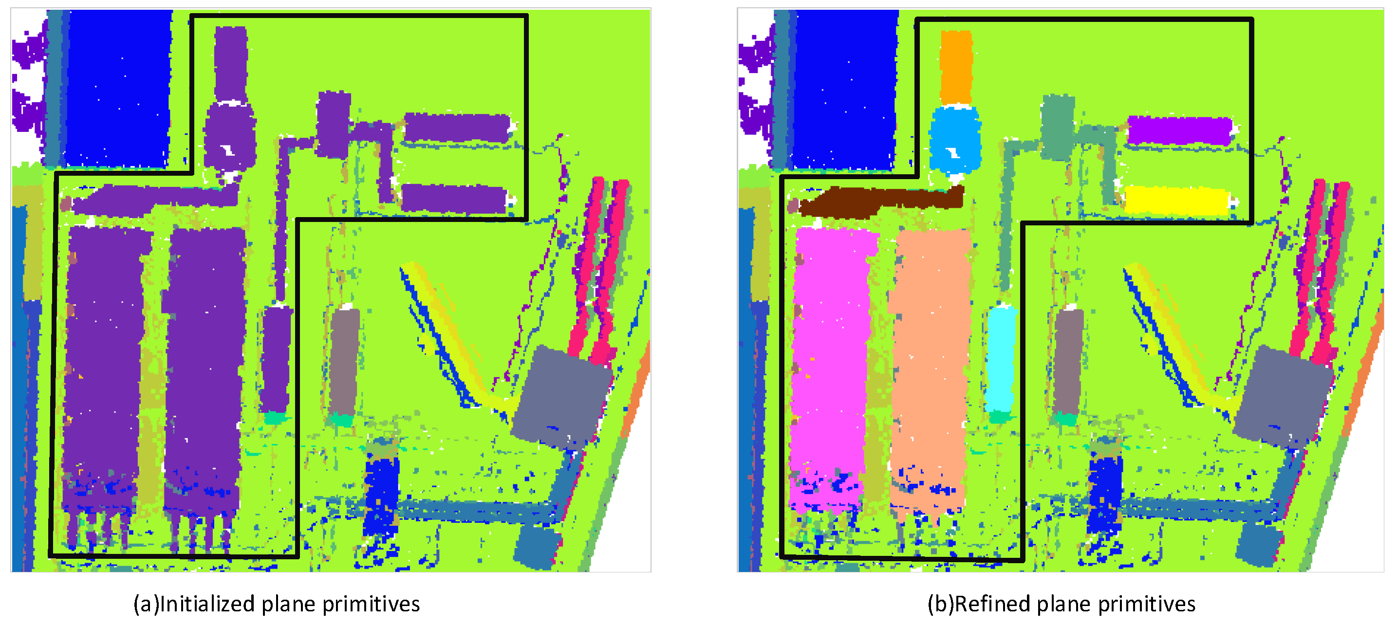
Figure 12 and Figure 13a show the planes after segmentation by the RANSAC algorithm. It can be seen that the RANSAC algorithm incorrectly divides the planes of different structures of the building into one plane, which is due to the difference in the height of the planes being less than the point-to-plane distance threshold. By resegmenting the planes, the missegmented planes are obtained optimized as shown in Figure 12 and Figure 13b. This optimization is made possible by the density-adaptive plane repartitioning of the DBSCAN algorithm.
Roof Plane Recognition. In order to highlight the advantages of the proposed roof plane recognition method based on the CSF algorithm, this section compares it with the roof plane recognition method based on the normal vector of the plane and the roof plane recognition method based on the normal vector of the plane and the combined judgment of the height, and the specific parameter settings and the results are shown in Table 3. According to the analysis in Table 3, the following analysis is made: The structure of building 1 is simple, and the roof planes can be recognized by the three methods. For buildings 2 and 3, the roof plane recognition method based on plane normal vector cannot accurately distinguish the roof from the façade of the balcony, steps and other structures and cannot recognize the vertical plane in the roof (such as the plane pointed by the black arrows in buildings 2 and 3), while the combined recognition method of plane normal vector and plane height needs to set up different plane heights for different buildings in order to exclude the accessory structure planes of the façade and add the vertical plane of the roof. In contrast, the CSF-based roof plane recognition method only needs to set common parameters to recognize the roof planes of buildings without setting different plane heights for different buildings.
The following conclusions can be drawn from the above analysis: (1) Usually, flat roofs, sloped roofs and elevations have different orientations, and roofs and elevations can be distinguished by the angle between the plane normal and the vertical direction. (2) In cases where the plane orientation of the accessory structure of the façade is the same as that of the roof plane or where there is a vertical plane in the roof plane, the roof plane identification method based on the plane normal vector may be erroneous. Although the combined plane normal vector and height recognition method can recognize the roof plane, it needs to set different heights according to the characteristics of the building. (3) The proposed CSF roof plane recognition method is unaffected by the absence of façade appendages and vertical planes in the roof, and it is more versatile as it does not require individual parameters for each building.
4.2.4. Reconstruction Models and Comparative Analysis
In this section, we introduce the building reconstruction steps, the methods used and their parameter settings, and show the reconstruction process and the final results, and compare and analyze the reconstructed model in this paper with the reconstructed model of PolyFit [16].
Reconstruction Parameter Settings. The methods and parameter settings used in each step of reconstruction are detailed in Table 4.
Reconstruction results and comparative analysis.
In Figure 14, Figure 15 and Figure 16, (a) represents the point cloud of the building, subfigure (b) represents the results of steps 1–7, subfigure (c) represents the final reconstructed wireframe model of the building, (d) and (e) represent the contrasting models, and (f) is the reference image.
By comparing the proposed building topology reconstruction method based on vertical plane reasoning with the building model reconstructed by the PolyFit [16] method, the following conclusions are drawn:
(1) The building model reconstruction method proposed in this paper mainly reconstructs the roof model of the building, while the 3D model of the building is obtained by stretching the outer contour of the roof to the ground. The proposed method mainly relies on the complete roof point cloud data, while the PolyFit building reconstruction method requires the complete point cloud data of the building, which limits the applicability of the PolyFit method to the reconstruction of point clouds of buildings in different scenes. However, the geometric accuracy (M2P) of the reconstructed model of the proposed method may be affected to some extent when dealing with buildings containing eave structures, and a comparison of the results of the reconstructed building model is shown in Figure 14d,e.
(2) When dealing with the point cloud plane defect problem, the proposed method can successfully reconstruct the building model as well as the PolyFit method, and the specific reconstruction results are shown in Figure 15. However, when the building point cloud has a plane missing, the proposed vertical plane inference method is still able to correctly reconstruct the building model (Figure 16a–d), whereas the model reconstructed by the PolyFit method has a plane error, such as the plane indicated by the red line in Figure 16e.
4.2.5. Evaluation and Analysis of Regional Reconstruction Model Accuracy
Figure 17, Figure 18 and Figure 19 show the results of the regional reconstructed images, regional point cloud data, and building point clouds overlaid with structured models, respectively. Table 5 provides statistics of specific values for P2M (point cloud to model) and M2P (model to point cloud).
For the two building types in the area, i.e., flat-roofed staggered-story buildings (e.g., Building 4 in Figure 18) and herringbone-roofed buildings (e.g., Buildings 2, 3, 5, etc., in Figure 18), there are fewer roof facets where they intersect. Therefore, the accuracy of the modeling depends more on the accuracy of the boundary fitting of the buildings and the geometric accuracy is poor.
For buildings 1, 8, 11 and 12 in Figure 18, the architectural structure is relatively more complex, with the same roof level containing multiple roof surfaces. The geometric accuracy of these buildings is better relative to the flat-roofed staggered-story buildings and herringbone-roofed buildings due to the restoration of the topological relationships between the planes.
Overall, topological reconstruction of the roof model was better in areas with plane intersecting building structures but performed slightly worse in fitting the boundaries of the flat-roof model and the herringbone model. The error of the model point cloud fitting was 0.31 m, and the geometric error was 0.25 m. In addition, some of the point cloud fitting errors for buildings with eaves were larger.
5. Conclusions
According to the experimental results, the proposed ELFA-RandLA-Net network shows higher performance relative to other methods, especially for semantic segmentation of buildings, the IoU value reaches 89.74%, which is 9.11% higher compared to RandLA-Net, and the performance improvement is significant. In this paper, we use the clustering method to monomer the building point cloud, which can effectively deal with buildings that exist at a certain distance, but there still exists the inability to automatically extract a single building point cloud for overlapping or closely neighboring buildings.
Our building topology reconstruction method, especially the inference method for the vertical plane of the roof, successfully solves the problem of failing to reconstruct the roof of a building due to the defective quality of the point cloud data of the vertical plane of the roof and ensures the correctness of the roof topology reconstruction. In addition, the reconstructed model is guaranteed to have a complete topological structure due to the restoration of the topological relationship of the building planes. For buildings with fewer intersecting roof planes, such as flat-roofed buildings, the accuracy of modeling is more dependent on the boundary fitting accuracy of the building, and the geometric accuracy of the building model is poor.
In the future, we plan to utilize the proposed roof plane recognition method to associate the semantic information of the building with the structured reconstruction in order to take a step further towards semantic reconstruction of buildings. In addition, we will further validate the effectiveness of the proposed reconstruction method for building reconstruction on low-density point cloud data and enhance the applicability of the method to different building types (e.g., cantilevered roofs).
Author Contributions
Conceptualization, Baoyun Guo, Na Sun, Yue Wang, and Yukai Yao; methodology, Na Sun and Yue Wang; software, Na Sun and Yukai Yao; validation, Na Sun and Yue Wang; formal analysis, Baoyun Guo; investigation, Yue Wang; writing—original draft preparation, Xiaokai Sun; writing—review and editing, Cailin Li; visualization, Yukai Yao, Na Sun and Yue Wang; supervision, Baoyun Guo and Na Sun. All authors have read and agreed to the published version of the manuscript.
Funding
The Project Supported by the Open Fund of Hubei Luojia Laboratory (No. 230100026) and Shandong Provincial Natural Science Foundation (No. ZR2022MD039).
Data Availability Statement
The data are not publicly available due to further research.
Acknowledgments
The authors express their gratitude to the Open Fund of Hubei Luojia Laboratory (Grant No. 230100026) and the Shandong Provincial Natural Science Foundation (Grant No. ZR2022MD039) for providing financial support for this research.
Conflicts of Interest
The authors declare no conflict of interest.
References
- Biljecki, F.; Stoter, J.; Ledoux, H.; Zlatanova, S.; Çöltekin, A. Applications of 3D city models: State of the art review. ISPRS Int. J. Geo-Inf. 2015, 4, 2842–2889. [Google Scholar] [CrossRef]
- Chen, R. The development of 3D city model and its applications in urban planning. In Proceedings of the 2011 19th International Conference on Geoinformatics, Shanghai, China, 24–26 June 2011; pp. 1–5. [Google Scholar]
- Jovanović, D.; Milovanov, S.; Ruskovski, I.; Govedarica, M.; Sladić, D.; Radulović, A.; Pajić, V. Building virtual 3D city model for smart cities applications: A case study on campus area of the university of novi sad. ISPRS Int. J. Geo-Inf. 2020, 9, 476. [Google Scholar] [CrossRef]
- Costantino, D.; Vozza, G.; Alfio, V.S.; Pepe, M. Strategies for 3D Modelling of Buildings from Airborne Laser Scanner and Photogrammetric Data Based on Free-Form and Model-Driven Methods: The Case Study of the Old Town Centre of Bordeaux (France). Appl. Sci. 2021, 11, 10993. [Google Scholar] [CrossRef]
- Li, Z.; Shan, J.; Sensing, R. RANSAC-based multi primitive building reconstruction from 3D point clouds. ISPRS J. Photogramm. Remote Sens. 2022, 185, 247–260. [Google Scholar] [CrossRef]
- Xiong, B.; Elberink, S.O.; Vosselman, G.; Sensing, R. A graph edit dictionary for correcting errors in roof topology graphs reconstructed from point clouds. ISPRS J. Photogramm. Remote Sens. 2014, 93, 227–242. [Google Scholar] [CrossRef]
- Xiong, B.; Jancosek, M.; Elberink, S.O.; Vosselman, G.; Sensing, R. Flexible building primitives for 3D building modeling. ISPRS J. Photogramm. Remote Sens. 2015, 101, 275–290. [Google Scholar] [CrossRef]
- Huang, W.; Jiang, S.; Jiang, W.J.S. A model-driven method for pylon reconstruction from oblique UAV images. Sensors 2020, 20, 824. [Google Scholar] [CrossRef] [PubMed]
- Chen, D.; Wang, R.; Peethambaran, J.; Sensing, R. Topologically aware building rooftop reconstruction from airborne laser scanning point clouds. IEEE Trans. Geosci. Remote Sens. 2017, 55, 7032–7052. [Google Scholar] [CrossRef]
- Li, H.; Xiong, S.; Men, C.; Liu, Y. Roof reconstruction of aerial point cloud based on BPPM plane segmentation and energy optimization. IEEE J. Sel. Top. Appl. Earth Obs. Remote Sens. 2023, 16, 5828–5848. [Google Scholar] [CrossRef]
- Li, L.; Song, N.; Sun, F.; Liu, X.; Wang, R.; Yao, J.; Cao, S.; Sensing, R. Point2Roof: End-to-end 3D building roof modeling from airborne LiDAR point clouds. ISPRS J. Photogramm. Remote Sens. 2022, 193, 17–28. [Google Scholar] [CrossRef]
- Sampath, A.; Shan, J.; Sensing, R. Segmentation and reconstruction of polyhedral building roofs from aerial lidar point clouds. IEEE Trans. Geosci. Remote Sens. 2009, 48, 1554–1567. [Google Scholar] [CrossRef]
- Wang, Y.; Xu, H.; Cheng, L.; Li, M.; Wang, Y.; Xia, N.; Chen, Y.; Tang, Y. Three-dimensional reconstruction of building roofs from airborne LiDAR data based on a layer connection and smoothness strategy. Remote Sens. 2016, 8, 415. [Google Scholar] [CrossRef]
- Huang, J.; Stoter, J.; Peters, R.; Nan, L. City3D: Large-scale building reconstruction from airborne LiDAR point clouds. Remote Sens. 2022, 14, 2254. [Google Scholar] [CrossRef]
- Liu, X.; Zhang, Y.; Ling, X.; Wan, Y.; Liu, L.; Li, Q. TopoLAP: Topology recovery for building reconstruction by deducing the relationships between linear and planar primitives. Remote Sens. 2019, 11, 1372. [Google Scholar] [CrossRef]
- Nan, L.; Wonka, P. Polyfit: Polygonal surface reconstruction from point clouds. In Proceedings of the IEEE International Conference on Computer Vision, Venice, Italy, 22–29 October 2017; pp. 2353–2361. [Google Scholar]
- Yang, S.; Cai, G.; Du, J.; Chen, P.; Su, J.; Wu, Y.; Wang, Z.; Li, J.; Sensing, R. Connectivity-aware Graph: A planar topology for 3D building surface reconstruction. ISPRS J. Photogramm. Remote Sens. 2022, 191, 302–314. [Google Scholar] [CrossRef]
- Cheng, R.; Razani, R.; Taghavi, E.; Li, E.; Liu, B. 2-s3net: Attentive feature fusion with adaptive feature selection for sparse semantic segmentation network. In Proceedings of the IEEE/CVF Conference on Computer Vision and Pattern Recognition, Nashville, TN, USA, 19–25 June 2021; pp. 12547–12556. [Google Scholar]
- Hou, Y.; Zhu, X.; Ma, Y.; Loy, C.C.; Li, Y. Point-to-voxel knowledge distillation for lidar semantic segmentation. In Proceedings of the IEEE/CVF Conference on Computer Vision and Pattern Recognition, New Orleans, LA, USA, 18–24 June 2022; pp. 8479–8488. [Google Scholar]
- Tang, H.; Liu, Z.; Zhao, S.; Lin, Y.; Lin, J.; Wang, H.; Han, S. Searching efficient 3d architectures with sparse point-voxel convolution. In Proceedings of the European Conference on Computer Vision, Glasgow, UK, 23–28 August 2020; pp. 685–702. [Google Scholar]
- Xu, J.; Zhang, R.; Dou, J.; Zhu, Y.; Sun, J.; Pu, S. Rpvnet: A deep and efficient range-point-voxel fusion network for lidar point cloud segmentation. In Proceedings of the IEEE/CVF International Conference on Computer Vision, Montreal, BC, Canada, 11–17 October 2021; pp. 16024–16033. [Google Scholar]
- Yan, X.; Gao, J.; Zheng, C.; Zheng, C.; Zhang, R.; Cui, S.; Li, Z. 2dpass: 2d priors assisted semantic segmentation on lidar point clouds. In Proceedings of the European Conference on Computer Vision, Tel Aviv, Israel, 23–27 October 2022; pp. 677–695. [Google Scholar]
- Hu, Q.; Yang, B.; Xie, L.; Rosa, S.; Guo, Y.; Wang, Z.; Trigoni, N.; Markham, A. Randla-net: Efficient semantic segmentation of large-scale point clouds. In Proceedings of the IEEE/CVF Conference on Computer Vision and Pattern Recognition, Seattle, WA, USA, 4–19 June 2020; pp. 11108–11117. [Google Scholar]
- Schnabel, R.; Wahl, R.; Klein, R. Efficient RANSAC for point-cloud shape detection. In Computer Graphics Forum; Blackwell Publishing Ltd.: Oxford, UK, 2007; pp. 214–226. [Google Scholar]
- El-Sayed, E.; Abdel-Kader, R.F.; Nashaat, H.; Marei, M. Plane detection in 3D point cloud using octree-balanced density down-sampling and iterative adaptive plane extraction. IET Image Process. 2018, 12, 1595–1605. [Google Scholar] [CrossRef]
- Rabbani, T.; Van Den Heuvel, F.; Vosselmann, G. Segmentation of point clouds using smoothness constraint. Int. Arch. Photogramm. Remote Sens. Spat. Inf. Sci. 2006, 36, 248–253. [Google Scholar]
- Wu, H.; Zhang, X.; Shi, W.; Song, S.; Cardenas-Tristan, A.; Li, K.; Sensing, R. An accurate and robust region-growing algorithm for plane segmentation of TLS point clouds using a multiscale tensor voting method. IEEE J. Sel. Top. Appl. Earth Obs. Remote Sens. 2019, 12, 4160–4168. [Google Scholar] [CrossRef]
- Zhu, X.; Liu, X.; Zhang, Y.; Wan, Y.; Duan, Y.; Sensing, R. Robust 3-D plane segmentation from airborne point clouds based on quasi-a-contrario theory. IEEE J. Sel. Top. Appl. Earth Obs. Remote Sens. 2021, 14, 7133–7147. [Google Scholar] [CrossRef]
- Albers, B.; Kada, M.; Wichmann, A. Automatic extraction and regularization of building outlines from airborne LiDAR point clouds. Int. Arch. Photogramm. Remote Sens. Spat. Inf. Sci. 2016, 41, 555–560. [Google Scholar] [CrossRef]
- Gilani, S.A.N.; Awrangjeb, M.; Lu, G. Segmentation of airborne point cloud data for automatic building roof extraction. GIScience Remote Sens. 2018, 55, 63–89. [Google Scholar] [CrossRef]
- Li, L.; Yan, H. Building contour regularization method based on ground LIDAR point cloud data. In Proceedings of the 2021 IEEE 4th Advanced Information Management, Communicates, Electronic and Automation Control Conference (IMCEC), Chongqing, China, 18–20 June 2021; pp. 1937–1941. [Google Scholar]
- Zhang, X.-Q.; Wang, H.; Shan, Y.-H.; Leng, L. Building Contour Extraction Based on LiDAR Point Cloud. In Proceedings of the ITM Web of Conferences, Wuhan, China, 24–26 March 2017; p. 10004. [Google Scholar]
- Edelsbrunner, H.; Kirkpatrick, D.; Seidel, R. On the shape of a set of points in the plane. IEEE Trans. Inf. Theory 1983, 29, 551–559. [Google Scholar] [CrossRef]
- Widyaningrum, E.; Peters, R.Y.; Lindenbergh, R. Building outline extraction from ALS point clouds using medial axis transform descriptors. Pattern Recognit. Lett. 2020, 106, 107447. [Google Scholar] [CrossRef]
- Kustra, J. Computing refined skeletal features from medial point clouds. Pattern Recognit. Lett. 2016, 76, 13–21. [Google Scholar] [CrossRef]
- Chen, D.; Zhang, L.; Mathiopoulos, P.T.; Huang, X. A methodology for automated segmentation and reconstruction of urban 3-D buildings from ALS point clouds. IEEE J. Sel. Top. Appl. Earth Obs. Remote Sens. 2014, 7, 4199–4217. [Google Scholar] [CrossRef]
- Verma, V.; Kumar, R.; Hsu, S. 3D building detection and modeling from aerial LIDAR data. In Proceedings of the 2006 IEEE Computer Society Conference on Computer Vision and Pattern Recognition (CVPR’06), New York, NY, USA, 17–22 June 2006; pp. 2213–2220. [Google Scholar]
- Wang, R.; Huang, S. Building3D: A Urban-Scale Dataset and Benchmarks for Learning Roof Structures from Point Clouds. In Proceedings of the IEEE/CVF International Conference on Computer Vision, Vancouver, BC, Canada, 18–22 June 2023. [Google Scholar]
- Xu, B. Deep learning guided building reconstruction from satellite imagery-derived point clouds. arXiv 2020, arXiv:2005.09223. [Google Scholar]
- Yu, D.; Ji, S.; Liu, J. Automatic 3D building reconstruction from multi-view aerial images with deep learning. ISPRS J. Photogramm. Remote Sens. 2021, 171, 155–170. [Google Scholar] [CrossRef]
- Yastikli, N.; Cetin, Z. Classification of raw LiDAR point cloud using point-based methods with spatial features for 3D building reconstruction. Arab. J. Geosci. 2021, 14, 146. [Google Scholar] [CrossRef]
- Sahebdivani, S.; Arefi, H.; Maboudi, M. Deep learning based classification of color point cloud for 3D reconstruction of interior elements of buildings. In Proceedings of the 2020 International Conference on Machine Vision and Image Processing (MVIP), Qom, Iran, 18–20 February 2020; pp. 1–6. [Google Scholar]
- Zhang, L.; Li, Z.; Li, A.; Liu, F.J.I.J.o.P.; Sensing, R. Large-scale urban point cloud labeling and reconstruction. ISPRS J. Photogramm. Remote Sens. 2018, 138, 86–100. [Google Scholar] [CrossRef]
- Zhou, Q.-Y.; Neumann, U. 2.5 d dual contouring: A robust approach to creating building models from aerial lidar point clouds. In Proceedings of the Computer Vision–ECCV 2010: 11th European Conference on Computer Vision, Heraklion, Crete, Greece, 5–11 September 2010; Proceedings, Part III 11. pp. 115–128. [Google Scholar]
- Qi, C.R.; Su, H.; Mo, K.; Guibas, L.J. Pointnet: Deep learning on point sets for 3d classification and segmentation. In Proceedings of the IEEE Conference on Computer Vision and Pattern Recognition, Honolulu, HI, USA, 21–26 July 2017; pp. 652–660. [Google Scholar]
- Kazhdan, M.; Bolitho, M.; Hoppe, H. Poisson surface reconstruction. In Proceedings of the Fourth Eurographics Symposium on Geometry Processing, Sardinia, Italy, 26–28 June 2006. [Google Scholar]
- Peterson, L. K-nearest neighbor. Scholarpedia 2009, 4, 1883. [Google Scholar] [CrossRef]
- Schubert, E.; Sander, J.; Ester, M.; Kriegel, H.P.; Xu, X. DBSCAN revisited, revisited: Why and how you should (still) use DBSCAN. ACM Trans. Database Syst. 2017, 42, 1–21. [Google Scholar] [CrossRef]
- Zhang, W.; Qi, J.; Wan, P.; Wang, H.; Xie, D.; Wang, X.; Yan, G.J.R.s. An easy-to-use airborne LiDAR data filtering method based on cloth simulation. Remote Sens. 2016, 8, 501. [Google Scholar] [CrossRef]
- Noto, M.; Sato, H. A method for the shortest path search by extended Dijkstra algorithm. In Proceedings of the SMC 2000 Conference Proceedings: 2000 IEEE International Conference on Systems, Man and Cybernetics: “Cybernetics Evolving to Systems, Humans, Organizations, and their Complex Interactions”, Nashville, TN, USA, 8–11 October 2010. [Google Scholar]
- Phan, A.V.; Le Nguyen, M.; Nguyen, Y.L.H.; Bui, L.T.J.N.N. Dgcnn: A convolutional neural network over large-scale labeled graphs. Neural Netw. 2018, 108, 533–543. [Google Scholar] [CrossRef]
- Boulch, A. ConvPoint: Continuous convolutions for point cloud processing. Comput. Graph. 2020, 88, 24–34. [Google Scholar] [CrossRef]
- Qiu, S.; Anwar, S.; Barnes, N. Semantic segmentation for real point cloud scenes via bilateral augmentation and adaptive fusion. In Proceedings of the IEEE/CVF Conference on Computer Vision and Pattern Recognition, Nashville, TN, USA, 19–25 June 2021; pp. 1757–1767. [Google Scholar]
Figure 1.
The proposed building reconstruction pipeline (only one building is selected to illustrate the workflow). (a) Input point cloud (point colors are rendered by elevation). (b) Semantically segmented building point cloud. (c) Monolithic building point cloud. (d) Single building point cloud. (e) Roof point cloud planes. (f) Building wireframe model, where the orange plane is the inferred vertical plane.

Figure 2.
Illustration of the ELFA-RandLA-Net network structure.

Figure 3.
Details of the enhanced local feature aggregation module.

Figure 4.
Building point cloud plane segmentation and roof plane recognition process. (a) The initial building plane primitive obtained by the RANSAC algorithm, where the plane pointed by the arrow in (a) is the incorrectly segmented plane; (b) the plane after resegmentation; (c) the shape of the roof of the building obtained by using the cloth simulation filtering algorithm, and the shape is represented by a mesh; (d) the automatically recognized roof plane.

Figure 5.
Building structured reconstruction pipeline. In subgraph (d), the light blue dots indicate the corresponding roof planes, while the straight lines between the dots indicate the existence of a neighboring relationship between the corresponding two roof planes. Different colors in the figure represent distinct planes of the buildings.

Figure 6.
Roof vertical plane inference, where the properties of the edges in (c) indicate the presence of vertical planes between plane nodes; the dark green plane in (d) is the inferred vertical plane. Different colors in the figure represent distinct planes of the buildings. In (a), the arrow points to the plane indicating the quality defects. In (b), the numbers represent the identification of building planes.

Figure 7.
A method for judging the adjacency of a plane, where the black lines in (b,c) are the adjacent sides of the polygon and the red lines are the polygon intersections.
Figure 7.
A method for judging the adjacency of a plane, where the black lines in (b,c) are the adjacent sides of the polygon and the red lines are the polygon intersections.

Figure 8.
Roof closed polygon, cyan lines are plane intersections in (a) and red lines are the edges of the roof polygon in (b), the orange and green points in (a,b) indicate inner and outer points, respectively.
Figure 8.
Roof closed polygon, cyan lines are plane intersections in (a) and red lines are the edges of the roof polygon in (b), the orange and green points in (a,b) indicate inner and outer points, respectively.

Figure 9.
The dataset for the central city of Dublin, where different colors indicate different semantic categories. The dataset consists of 13 different sections.
Figure 9.
The dataset for the central city of Dublin, where different colors indicate different semantic categories. The dataset consists of 13 different sections.

Figure 10.
A comparative example of network predictions, where the color information corresponding to the different categories can be found in Figure 11a.
Figure 10.
A comparative example of network predictions, where the color information corresponding to the different categories can be found in Figure 11a.

Figure 12.
Example 1 of the segmentation and optimization results of the RANSAC algorithm, where the planes indicated by the arrows in (a,b) denote the missegmented plane to be optimized and the optimized plane, respectively.
Figure 12.
Example 1 of the segmentation and optimization results of the RANSAC algorithm, where the planes indicated by the arrows in (a,b) denote the missegmented plane to be optimized and the optimized plane, respectively.

Figure 13.
Example 2 of the segmentation and optimization results of the RANSAC algorithm, where the boxed planes in (a,b) denote the missegmented plane to be optimized and the optimized plane, respectively. Different colors in the figure represent distinct planes of the buildings.
Figure 13.
Example 2 of the segmentation and optimization results of the RANSAC algorithm, where the boxed planes in (a,b) denote the missegmented plane to be optimized and the optimized plane, respectively. Different colors in the figure represent distinct planes of the buildings.

Figure 14.
Reconstruction results for Building 1. The red points in (b) represent the initial roof surface vertices, while the black lines indicate the neighboring relationships between the planes; the green points in (c) represent the corrected roof surface vertices.
Figure 14.
Reconstruction results for Building 1. The red points in (b) represent the initial roof surface vertices, while the black lines indicate the neighboring relationships between the planes; the green points in (c) represent the corrected roof surface vertices.

Figure 15.
Reconstruction results for Building 2. The red points in (b) represent the initial roof surface vertices, the black lines indicate the neighborhood between the planes, and the blue is the fitted plane; the green points in (c) represent the corrected roof surface vertices.
Figure 15.
Reconstruction results for Building 2. The red points in (b) represent the initial roof surface vertices, the black lines indicate the neighborhood between the planes, and the blue is the fitted plane; the green points in (c) represent the corrected roof surface vertices.

Figure 16.
Reconstruction results for building 3. The red points in (b) represent the initial roof surface vertices, the black lines indicate the neighborhood between the planes, and the blue is the fitted plane; the green points in (c) represent the corrected roof surface vertices.
Figure 16.
Reconstruction results for building 3. The red points in (b) represent the initial roof surface vertices, the black lines indicate the neighborhood between the planes, and the blue is the fitted plane; the green points in (c) represent the corrected roof surface vertices.

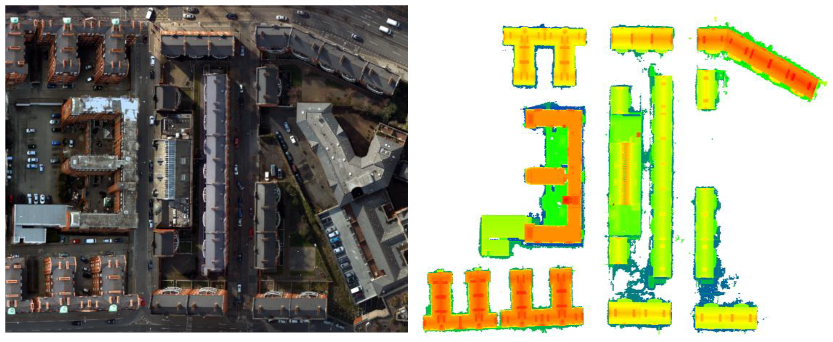
Figure 17.
Regional reconstructed orthophoto and point cloud.

Figure 18.
The reconstruction results of the buildings in the region, where the planes circled in red are the poorly fitted planes to the point cloud. In order to present the reconstruction of the buildings more clearly, we transformed the wireframe model into a polyhedral model and used different colors to represent the different planes of the buildings. In the figure, the different planes of the building are shown in different colors.

Figure 19.
Building point cloud overlaid with structured model showing results, where the planes circled in red are the poorly fitted planes to the point cloud.
Figure 19.
Building point cloud overlaid with structured model showing results, where the planes circled in red are the poorly fitted planes to the point cloud.


Table 1.
Semantic segmentation results of different methods on Dublin data (%).
| OA | Precision | mIoU | Building | Grass | Sidewalk | Street | Bush | Tree | Undefined | ||
|---|---|---|---|---|---|---|---|---|---|---|---|
| DGCNN [51] | 74.12 | 42.8 | 53.34 | 41.66 | 75.63 | 30.56 | 15.64 | 32.45 | 0.37 | 92.48 | 44.52 |
| ConvPoint [52] | 75.46 | 50.5 | 60.12 | 49.50 | 78.15 | 38.52 | 38.71 | 44.83 | 0.80 | 93.83 | 51.63 |
| RandLA-Net [23] | 77.74 | 52.0 | 62.48 | 51.01 | 80.63 | 43.68 | 37.06 | 46.05 | 1.52 | 91.64 | 56.48 |
| Qiu [53] | 78.94 | 55.8 | 64.76 | 54.34 | 85.44 | 45.12 | 44.12 | 52.12 | 3.25 | 92.45 | 57.63 |
| Ours | 79.02 | 55.9 | 63.02 | 54.49 | 89.74 | 44.02 | 42.54 | 51.75 | 3.63 | 92.78 | 57.01 |
Table 2.
Accuracy evaluation of different methods on SemanticKITTI dataset (%).
| Model | Params(M) | mIoU | Car | Bicycle | Motorcycle | Truck | Other Vehicle | Person | Bicyclist | Motorcyclist | Road | Parking | Sidewalk | Other Ground | Building | Fence | Vegetation | Trunk | Terrain | Pole | Traffic Sign |
|---|---|---|---|---|---|---|---|---|---|---|---|---|---|---|---|---|---|---|---|---|---|
| PointNet | 3.0 | 14.6 | 46.3 | 1.3 | 0.3 | 0.1 | 0.8 | 0.2 | 0.2 | 0.0 | 61.6 | 15.8 | 35.7 | 1.4 | 41.4 | 12.9 | 31.0 | 4.6 | 17.6 | 2.4 | 3.7 |
| SPG | 0.3 | 17.4 | 49.3 | 0.2 | 0.2 | 0.1 | 0.8 | 0.3 | 2.7 | 0.1 | 45.0 | 0.6 | 28.5 | 0.6 | 64.3 | 20.8 | 48.9 | 27.2 | 24.6 | 15.9 | 0.8 |
| PointNet++ | 6.0 | 20.1 | 53.7 | 1.9 | 0.2 | 0.9 | 0.2 | 0.9 | 1.0 | 0.1 | 72.0 | 18.7 | 41.8 | 5.6 | 62.3 | 16.9 | 46.5 | 0.9 | 30.0 | 6.0 | 8.9 |
| TangentConv | 0.4 | 40.9 | 90.8 | 2.7 | 16.5 | 15.2 | 12.1 | 23.0 | 28.4 | 8.1 | 83.9 | 33.4 | 63.9 | 15.4 | 83.4 | 49.0 | 79.5 | 49.3 | 58.1 | 35.8 | 28.5 |
| RandLA-Net | 1.2 | 53.9 | 94.2 | 26.0 | 25.8 | 40.1 | 38.9 | 49.2 | 48.2 | 7.2 | 90.7 | 60.3 | 73.7 | 20.4 | 86.9 | 56.3 | 81.4 | 61.3 | 66.8 | 49.2 | 47.7 |
| SPVNAS | 12.5 | 67.0 | 97.2 | 50.6 | 50.4 | 56.6 | 58.0 | 67.4 | 67.1 | 50.3 | 90.2 | 67.6 | 75.4 | 21.8 | 91.6 | 66.9 | 86.1 | 73.4 | 71.0 | 64.3 | 67.3 |
| AF2-S3Net | - | 69.7 | 94.5 | 65.4 | 86.8 | 39.2 | 41.1 | 80.7 | 80.4 | 74.3 | 91.3 | 68.8 | 72.5 | 53.5 | 87.9 | 63.2 | 70.2 | 68.5 | 53.7 | 61.5 | 71.0 |
| RPVNet | 24.8 | 70.3 | 97.6 | 68.4 | 68.7 | 44.2 | 61.1 | 75.9 | 74.4 | 73.4 | 93.4 | 70.3 | 80.7 | 33.3 | 93.5 | 72.1 | 86.5 | 75.1 | 71.7 | 64.8 | 61.4 |
| PVKD | - | 71.2 | 97.0 | 67.9 | 69.3 | 53.5 | 60.2 | 75.1 | 73.5 | 50.5 | 91.8 | 70.9 | 77.5 | 41.0 | 92.4 | 69.4 | 86.5 | 73.8 | 71.9 | 64.9 | 65.8 |
| 2DPASS | _ | 72.9 | 97.0 | 63.6 | 63.4 | 61.1 | 61.5 | 77.9 | 81.3 | 74.1 | 89.7 | 67.4 | 74.7 | 40.0 | 93.5 | 72.9 | 86.2 | 73.9 | 71.0 | 65.0 | 70.4 |
| Ours | 1.5 | 58.0 | 94.7 | 50.4 | 40.8 | 36.1 | 37.0 | 52.1 | 54.3 | 10.4 | 91.4 | 59.8 | 75.4 | 21.4 | 94.1 | 55.4 | 83.4 | 61.8 | 68.3 | 52.1 | 58.8 |
Table 3.
Parameter settings and results of different roof plane identification methods.
| Collection of Building Planes | Based on Plane Normal Vectors | Based on Plane Normal Vectors and Heights | Based on CSF Algorithm | |
|---|---|---|---|---|
| B1 |  |  angle > . |  angle > and height > 8 m. |  cloth resolution = 0.5, classification threshold = 0.5. |
| B2 |  |  angle > . |  angle > and height > 10 m. |  cloth resolution = 0.5, classification threshold = 0.5. |
| B3 |  |  angle > . |  angle > and height > 20 m. |  cloth resolution = 0.5, classification threshold = 0.5. |
Table 4.
Methods used for building reconstruction and their parameterization.
| Building Reconstruction Steps | Corresponding Methods | Parameter Setting |
|---|---|---|
| Step1: building plane segmentation | RANSAC plane segmentation | Distance threshold from point to plane 0.1 m, minimum number of points 10, iteration number 500. |
| Step2: building plane optimization | DBSCAN plane optimization | Search radius 0.15 m, minimum number of points 3. |
| Step3: roof plane identification | CSF algorithm to recognize roof planes | cloth resolution 0.3 m, classification threshold 0.5 m. |
| Step4: roof plane initial boundary vertex acquisition | Alpha shape extracts contour points and RANSAC fits straight lines. | Alpha parameter 0.3, distance threshold for straight line fitting is 0.3 m. |
| Step5: roof vertical plane reasoning | Fit the plane according to the structural characteristics of the building | None |
| Step6: roof plane adjacency judgment | Set the distance threshold to judge the adjacency between the planes | The distance threshold is generally set to 3–5 times the average point cloud spacing. |
| Step7: roof topology reconstruction | Intersect planes to find intersection points, intersect straight lines. | None |
| Step8: building model reconstruction | Stretch the outer contour of the roof to the ground | None |
Table 5.
Regional model accuracy statistics.
| Max | Mean | RMS | |
|---|---|---|---|
| P2M (m) | 0.67 | 0.31 | 0.42 |
| M2P (m) | 0.39 | 0.25 | 0.26 |
Note: Max, Mean, and RMS are the maximum, mean, and median error, respectively.
Disclaimer/Publisher’s Note: The statements, opinions and data contained in all publications are solely those of the individual author(s) and contributor(s) and not of MDPI and/or the editor(s). MDPI and/or the editor(s) disclaim responsibility for any injury to people or property resulting from any ideas, methods, instructions or products referred to in the content. |
© 2024 by the authors. Licensee MDPI, Basel, Switzerland. This article is an open access article distributed under the terms and conditions of the Creative Commons Attribution (CC BY) license (https://creativecommons.org/licenses/by/4.0/).
Share and Cite
MDPI and ACS Style
Sun, X.; Guo, B.; Li, C.; Sun, N.; Wang, Y.; Yao, Y. Semantic Segmentation and Roof Reconstruction of Urban Buildings Based on LiDAR Point Clouds. ISPRS Int. J. Geo-Inf. 2024, 13, 19. https://doi.org/10.3390/ijgi13010019
AMA Style
Sun X, Guo B, Li C, Sun N, Wang Y, Yao Y. Semantic Segmentation and Roof Reconstruction of Urban Buildings Based on LiDAR Point Clouds. ISPRS International Journal of Geo-Information. 2024; 13(1):19. https://doi.org/10.3390/ijgi13010019
Chicago/Turabian StyleSun, Xiaokai, Baoyun Guo, Cailin Li, Na Sun, Yue Wang, and Yukai Yao. 2024. "Semantic Segmentation and Roof Reconstruction of Urban Buildings Based on LiDAR Point Clouds" ISPRS International Journal of Geo-Information 13, no. 1: 19. https://doi.org/10.3390/ijgi13010019
Note that from the first issue of 2016, this journal uses article numbers instead of page numbers. See further details here.