


Enhancing Crop Classification Accuracy through Synthetic SAR-Optical Data Generation Using Deep Learning


Faculty of Civil Engineering and Transportation, University of Isfahan, Isfahan 8174673441, Iran
*
Author to whom correspondence should be addressed.
ISPRS Int. J. Geo-Inf. 2023, 12(11), 450; https://doi.org/10.3390/ijgi12110450
Submission received: 23 August 2023
/
Revised: 30 September 2023
/
Accepted: 25 October 2023
/
Published: 2 November 2023
(This article belongs to the Special Issue Unlocking the Power of Geospatial Data: Semantic Information Extraction, Ontology Engineering, and Deep Learning for Knowledge Discovery)
Abstract
:Crop classification using remote sensing data has emerged as a prominent research area in recent decades. Studies have demonstrated that fusing synthetic aperture radar (SAR) and optical images can significantly enhance the accuracy of classification. However, a major challenge in this field is the limited availability of training data, which adversely affects the performance of classifiers. In agricultural regions, the dominant crops typically consist of one or two specific types, while other crops are scarce. Consequently, when collecting training samples to create a map of agricultural products, there is an abundance of samples from the dominant crops, forming the majority classes. Conversely, samples from other crops are scarce, representing the minority classes. Addressing this issue requires overcoming several challenges and weaknesses associated with the traditional data generation methods. These methods have been employed to tackle the imbalanced nature of training data. Nevertheless, they still face limitations in effectively handling minority classes. Overall, the issue of inadequate training data, particularly for minority classes, remains a hurdle that the traditional methods struggle to overcome. In this research, we explore the effectiveness of a conditional tabular generative adversarial network (CTGAN) as a synthetic data generation method based on a deep learning network, for addressing the challenge of limited training data for minority classes in crop classification using the fusion of SAR-optical data. Our findings demonstrate that the proposed method generates synthetic data with a higher quality, which can significantly increase the number of samples for minority classes, leading to a better performance of crop classifiers. For instance, according to the G-mean metric, we observed notable improvements in the performance of the XGBoost classifier of up to 5% for minority classes. Furthermore, the statistical characteristics of the synthetic data were similar to real data, demonstrating the fidelity of the generated samples. Thus, CTGAN can be employed as a solution for addressing the scarcity of training data for minority classes in crop classification using SAR–optical data.
1. Introduction
Cropland classification using remote sensing data has been among the hot and remarkable topics of research in the last two decades. Remotely sensed data acquired by synthetic aperture radar (SAR) and optical sensors have an undeniable role in estimating the area under cultivation and determining the crop yield through preparing a reliable crop map. The fusion of SAR and optical data can greatly help to improve classification accuracy and achieve more comprehensive information.
The RapidEye satellite a relatively high-resolution optical satellites that has been used in several recent studies for agricultural applications, especially crop mapping [1,2,3,4,5,6]. The spectral bands of RapidEye were specially designed for applications related to vegetation analysis and have provided improved indexing capabilities for extracting crop types [4]. On the other hand, the uninhabited aerial vehicle synthetic aperture radar (UAVSAR) radar satellite has also been one of the most widely used radar sensors in the field of crop mapping in the last few years [7,8,9,10,11,12,13]. In addition to providing high spatial resolution pixels, this sensor has all four polarizations. Therefore, it is possible to extract coherent and incoherent decomposition parameters related to vegetation and crop types. The fusion of both sensors has shown good potential for improving the accuracy of crop mapping in different studies [14,15,16].
Agricultural regions have distinct cultivation patterns, with each region typically characterized by one or two predominant crops, while other crops are less prevalent. Consequently, the availability of training data for all classes, particularly minority crops, is limited. This scarcity poses a challenge for conventional classifiers, as they struggle to accurately differentiate between minority and dominant classes. Consequently, classes with insufficient training samples often experience misclassification. For instance, previous research [17] demonstrated that the maximum likelihood and fully connected classifiers exhibited poor performance when trained on datasets with insufficient samples compared to datasets with sufficient samples. In summary, the heavy emphasis in agricultural regions on a small set of major crops leads to an unequal distribution of training data, resulting in insufficient data for minority crops. This imbalance negatively impacts the performance of conventional classifiers, resulting in misclassification of minority classes.
In order to address the challenge of insufficient training data, various methods can be employed in the data preprocessing stage. These methods aim to mitigate the impact of limited samples on classifier performance. For instance, the random under-sampling (RUS) method attempts to equalize the influence of few training samples across all classes by randomly removing samples from the majority classes [18]. However, this approach carries the risk of discarding potentially valuable and informative samples that could benefit the classifier. Conversely, the random over-sampling (ROS) method aims to artificially increase the sample size of minority classes by duplicating samples. While this technique may help balance the class distribution, it also introduces the possibility of overfitting the classifier, due to the generation of redundant and uninformative data [18]. It is important to note that both the RUS and ROS methods have their limitations and potential drawbacks. RUS may result in sample loss, while ROS can lead to overfitting.
To solve such problems, the synthetic minority oversampling technique (SMOTE) was proposed, in which synthetic data are created based on the feature space similarities between minority class samples and using linear interpolation between K existing samples [19]. This method has shown good performance in several studies [19,20,21]. However, this algorithm has also weaknesses. Specifically, SMOTE can be divided into two parts. The first part is the strategy of selecting the available samples to be used in the synthetic data generation stage. Since SMOTE considers the importance of all samples of the minority class to be the same, the generated synthetic data are always accompanied by noise. The second part of SMOTE is the linear interpolation strategy for synthetic data generation. This strategy leads to the generation of almost duplicated data, which will cause overfitting in the classifier training process. Table 1 summarizes the previous studies that used data generation methods to improve the accuracy of land use and land cover classification.
Recent advances in deep generative networks have created many possibilities in the field of synthetic data generation. These networks try to learn the probability distribution of real data and produce high-quality synthetic samples. Typically, generative models have illustrated good performance in the image and text domains, but they have not achieved much success in producing structured (tabular) synthetic data. In recent years, several studies have focused on improving the performance of generative models, especially generative adversarial networks (GAN), for structured data [27]. One of the most important challenges is often the non-Gaussian distribution of features in tabular data [28]. As a solution, conditional tabular GAN (CTGAN) has been developed, to generate synthetic data by considering the distribution of input features. In the architecture of the CTGAN network, a new normalization method is used to overcome non-Gaussian distributions. Thus, CTGAN can potentially be employed for synthetic feature generation in the case of insufficient training data for the crop classification task. This paper aimed to explore the potential of the CTGAN network in addressing the challenge of crop classification using unbalanced tabular samples that comprise optical and SAR polarimetric features. While previous studies have examined the capabilities of the CTGAN network in various data science domains, this study focused on investigating the network’s effectiveness in mitigating the impact of insufficient training data on agricultural product classification using SAR-optical derived features. The simultaneous integration of optical and SAR data has the potential to yield significant improvements in classification accuracy. By combining the unique strengths of these two data modalities, such as the spectral information from optical data and the structural information from SAR data, we can obtain a more comprehensive understanding of the target objects or land cover classes. This fusion of information enhances the discriminative power of the classification models and enables them to capture a wider range of features and characteristics. Furthermore, this study aimed to explore the capabilities of the CTGAN model in generating synthetic data, using both optical and SAR images. CTGAN, as a powerful deep learning-based generative model, has shown promise for generating realistic synthetic data that closely resemble the distribution of the original data. By leveraging this capability, we can effectively augment the training dataset with synthetic samples, thereby increasing data diversity and balancing class distributions. This approach has the potential to address the challenge of limited or imbalanced training data, ultimately improving the classification performance. The investigation of simultaneously integrating optical and SAR data, along with the generation of synthetic data using CTGAN, holds tremendous potential for advancing classification tasks, enhancing accuracy, and improving the effectiveness of analyzing complex Earth observation datasets. This combined approach offers a promising avenue for achieving more precise and reliable results, enabling researchers to extract valuable insights from diverse data sources and address challenges such as imbalanced or limited training data. By leveraging the complementary nature of optical and SAR data and harnessing the synthetic data generation capabilities of CTGAN, we can create a comprehensive dataset that captures the unique characteristics of both modalities and enhances the performance of classification models. Ultimately, this research direction has the potential to significantly contribute to the accuracy, robustness, and reliability of classification analyses in the field of earth observation.
This manuscript consists of several sections: the literature review and the objective of this investigation were introduced earlier. In the following, the study area and the dataset are introduced in Section 2.1. The details of the proposed method and experimental settings are explained in Section 2.2 and Section 2.3, respectively. Section 3 presents the results of experiments. Finally, the paper is concluded with a discussion of the achieved results.
2. Materials and Methods
2.1. Dataset and Study Area
The study area in this research was an agronomical area of Winnipeg, Manitoba, Canada (see Figure 1). The research used the fused data from bi-temporal optical and PolSAR images. The optical and PolSAR images were acquired from the RapidEye and UAVSAR sensors on 5 and 14 July 2012. The spectral bands of the RapidEye images were blue (B), green (G), red (R), near-infrared (NIR), and red-edge (RE), with a spatial resolution of about 5 m. The UAVSAR images had four polarizations at L-band frequency, with a spatial resolution of about 15 m.
The Soil Moisture Active Passive Validation Experiment 2012 (SMAPVEX 2012) campaign was conducted for the calibration and validation of the National Aeronautics and Space Administration (NASA)’s SMAP satellite over 43 days during the summer of 2012 [29]. During this operation, the crop type labels of this dataset were collected from the study area, including seven classes: broadleaf, canola, corn, oats, peas, soybeans, and wheat.
Table 2 presents the imbalance ratios (IR) in the utilized dataset, which measure the disparity in sample distribution. The IR is calculated as the ratio of to , where represents the number of samples in each class and represents the number of samples in the majority class. It is evident that there is an imbalanced distribution among the samples across different classes. In particular, the peas and broadleaf classes are identified as minority classes, while the remaining classes are categorized as majority classes.
2.2. Methodology
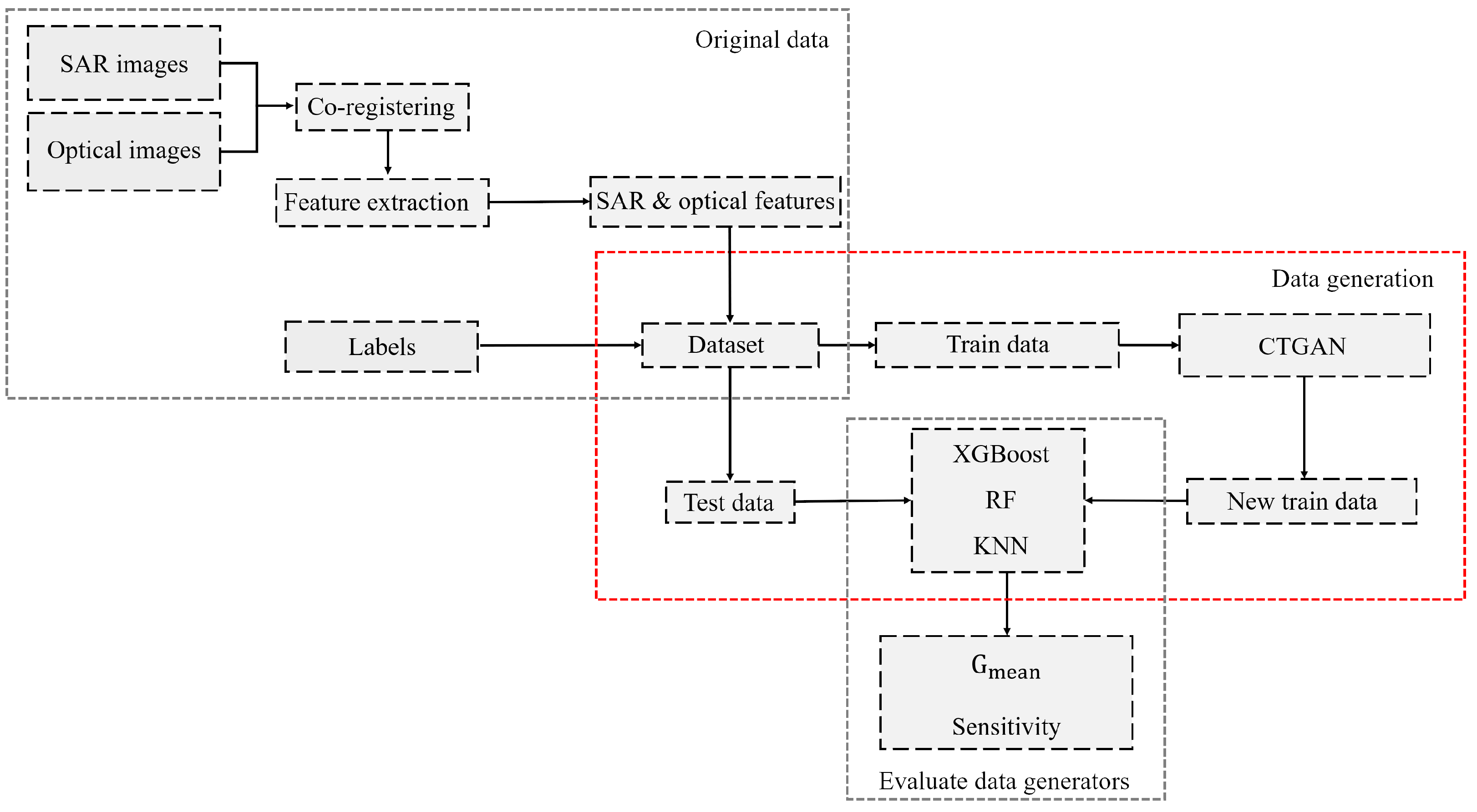
The detrimental impact of insufficient training samples in the minority classes on classifier performance has been highlighted in the introduction. This study investigated the potential of the CTGAN network in addressing this issue, specifically in the context of agricultural product classification using SAR and optical polarimetric features. The research process is depicted in Figure 2, outlining the key steps involved. Initially, preprocessing was applied to the SAR and optical images. Before any process, it is necessary to co-register SAR and optical images. These two image sources were co-registered with a linear polynomial for geometrical rectifying and the nearest neighbor method for gray level interpolation [30]. Then, various features were extracted from the optical and SAR images in the location of sample data (training and testing). More details are explained in the next section. After feature extraction and data preparation, the imbalanced and insufficient training data were fed into the CTGAN to rebalance the dataset by generating synthetic samples to increase the sample data of the minority classes. The resulting new dataset was then utilized for hyperparameter tuning of the different classifiers. Notably, the test samples were separated in advance and were not involved in the process of hyperparameter tuning or training the models.Finally, the quality of the generated synthetic data was evaluated by assessing the performance of the trained classifiers on the independent test data. This evaluation served to illustrate the effectiveness of the CTGAN network in addressing the challenge of insufficient training data for minority classes in agricultural product classification. More details of each step are given in the following sections.
2.2.1. Optical and Polarimetric Feature Extraction
In this research, we extracted features from SAR and optical imagery according to the methodology presented in [15]. Table 3 and Table 4 present the optical and polarimetric features, respectively. The optical features for RapidEye image included 5 spectral channels, 17 vegetation indices, and 16 textural indicators, which made a total of 38 features. Spectral channels were blue (B), green (G), red (R), red edge (RE), and near infrared red (NIR). Vegetation indices were the normalized difference vegetation index (NDVI), simple ratio (SR), enhanced vegetation index (EVI), red-green ratio index (RGRI), atmospherically resistant vegetation index (ARVI), soil adjusted vegetation index (SAVI), normalized difference greenness index (NDGI), green NDVI (gNDVI), modified triangular vegetation index (MTVI2), red-edge normalized difference vegetation index (), red-edge simple ratio (), red-edge normalized difference greenness index (), red-edge triangular vegetation index (), red-edge NDVI (RNDVI), transformed chlorophyll absorption in reflectance index (TCARI), triangular vegetation index (TVI), and red-edge ratio 2 (RRI2). In addition, eight main parameters of the gray level concurrence matrix (GLCM) of pc1 and pc2, i.e., the mean (), variance (), homogeneity (HOM), contrast (CON), dissimilarity (DIS), entropy (ENT), angular second moment (ASM), and correlation (COR) were used to describe the textural information. These features provide valuable information about vegetation reflectance in the visible and infrared regions of the electromagnetic spectrum or the spatial characteristics of the crop types [6,31].
The polarimetric features for each UAVSAR image included 6 backscattering intensities, 6 polarization ratios, 6 ratio values, 6 correlation coefficients, 12 Cloud and Pottier parameters, 2 Pauli parameters, 2 Krogager parameters, 2 Freeman–Durden parameters, and 4 Yamaguchi parameters, for a total of 46 features. Note that H, A, and are the entropy, anisotropy, and alpha angle, respectively. , , and are the eigenvalues of the coherency matrix (T); is the pedestal height; and RVI is the radar vegetation index. The polarimetric features give information about the physical and structural properties and also the scattering mechanisms of the various crop types [32].
2.2.2. Machine Learning Classifiers
Classifiers based on machine learning have received much attention in past studies, especially in the field of remote sensing [33,34,35,36]. These algorithms have a good ability to model complex classes and understand different input features. In addition, they don not require any initial assumptions about the data distribution. In general, these algorithms are more accurate than the traditional parametric methods, especially in the face of high-dimensional data [37]. In this research, three algorithms, i.e., random forest (RF), extreme gradient boosting (XGBoost), and K nearest neighbor (KNN) were used to investigate the performance of the CTGAN network in generating synthetic SAR-optical features.
RF utilizes the bagging method for training, where base learners (decision trees) are trained independently. In this approach, random sampling with replacement is performed, meaning that data points are randomly selected from the training set. Consequently, a training sample may be selected multiple times within the chosen data. The majority vote of each decision tree’s output determines the final output class. By aggregating decision trees, RF is robust against overfitting, capable of identifying outliers, and can assess the importance of input variables. However, by raising the number and complexity of trees, the training and prediction time of the model also increase [38].
The XGBoost algorithm, based on gradient-boosted decision trees (GBDT), is another popular machine learning algorithm. It leverages the errors from previous iterations and enhances the importance and weight of incorrectly predicted instances in subsequent iterations. XGBoost incorporates regularization in the cost function to avoid overfitting and employs parallel processing during training, resulting in faster processing and improved accuracy. Each tree in this algorithm generates an output based on different independent variables. After constructing the trees, the majority of the predicted classes determine the class of the input data [39].
KNN is a lazy learning algorithm that operates based on nearest neighbors. It calculates the distance between the test sample and all training samples, selects the K closest samples based on distance, and determines the dominant class among these K samples as the class of the test sample [40].
2.2.3. Synthetic Data Generation
The introduction highlighted the negative impact of insufficient training samples on the performance of various classifiers. This issue leads to reduced effectiveness of the minority classes in minimizing the loss function during training, resulting in classifier bias towards majority classes [41]. To address this challenge, different methods are employed, including random sampling techniques, such as ROS and RUS. The strengths and weaknesses of these methods were previously discussed in the Introduction. Another popular method for generating synthetic data for minority classes is SMOTE. This technique generates artificial samples along the connecting line between K real samples within the minority classes. Previous studies have successfully utilized SMOTE for synthetic data generation [19,22,42]. However, this method still suffers from certain problems, such as generating outlier data. Moreover, there are scenarios where using linear interpolation in the SOMTE method will cause the generation of duplicate data and the occurrence of problems such as overlearning [22].
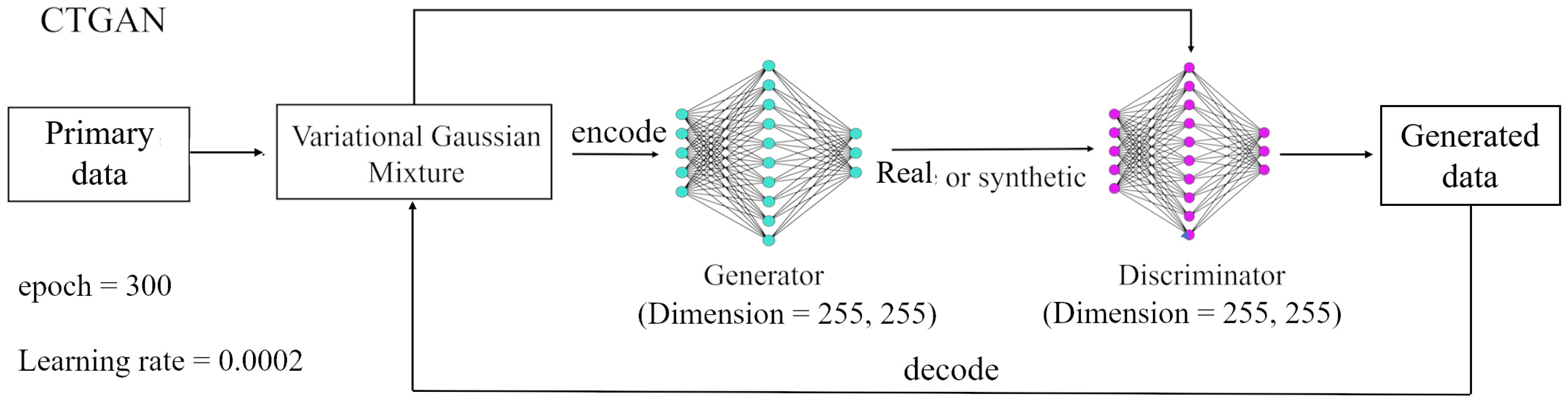
Recently, GAN networks have been employed for generating various types of synthetic data. GAN networks include two parts, a generator and a discriminator, which learn the distribution of data through an adversarial training process. The task of the generator is to generate synthetic data assuming a Gaussian distribution for the real data. The discriminator is responsible for distinguishing synthetic data produced by the generator from real data. When the generator can defeat the discriminator, the GAN network will be able to produce synthetic data similar to the real data. However, these networks encounter challenges in generating desirable synthetic samples in the case of a non-Gaussian distribution of tabular datasets. To diminish this weakness, the CTGAN network was proposed. CTGAN is a special type of GAN, designed to generate synthetic structured (tabular) data. Despite the architectural similarities of CTGAN with other GANs, there are also key differences between these networks. First, CTGAN was specifically designed for generating synthetic tabular data, which includes both continuous and categorical variables organized in a tabular format. Second, CTGAN supports conditional data generation, which means users can specify conditions for generating synthetic data of a particular variable. Third, CTGAN uses categorical embeddings to represent categorical variables in the generated synthetic data. This allows CTGAN to effectively handle discrete categorical variables in tabular data. Other GANs may not have specific mechanisms to handle categorical variables or may require additional preprocessing or encoding techniques [28,43,44,45]. Figure 3 illustrates the overall structure of CTGAN, which includes novel preprocessing techniques to improve GAN performance in tabular data generation. Tabular data distributions may be non-Gaussian. This can cause GANs to struggle with the “vanishing gradient” problem during training. To address this, CTGAN first estimates the underlying distribution of each feature using a variational Gaussian mixture model (VGMM). VGMM represents the overall distribution as a weighted combination of multiple Gaussian components, each with its own mean and covariance. This models multi-modal distributions more flexibly than a single Gaussian component. The estimated VGMM distribution is then used to normalize each feature through “encoding”. The encoded data have a standardized distribution that helps the GAN training converge. The generator produces synthetic samples in this normalized space. After training, a “decoding” step transforms the generated data back to the original distribution through the reverse of encoding transformations. This preprocessing allows CTGAN to handle complex, non-Gaussian tabular datasets, while stabilizing GAN training. The end-to-end framework can generate high-quality synthetic samples in the native distribution of the real data [28,43].
CTGAN network training is based on the following loss function:
where and are the loss functions for the discriminator and the generators, respectively; is the output of the discriminator for real data; is the output of the discriminator for synthetic data; H is the cross-entropy score; and m denotes the number of synthetic samples [28,43].
2.3. Experimental Setups
During the training process of all algorithms, 10% of the dataset was allocated as the training dataset, while the remaining data served as the test dataset. To determine the optimal hyperparameters for each classifier, we employed the random search algorithm combined with a K-Fold cross-validation strategy. Specifically, we set the value of K to 3, indicating that the training dataset was divided into three subsets (folds) of approximately equal size. During the random search process, different combinations of hyperparameters were randomly sampled from predefined ranges for each classifier. These hyperparameters included parameters such as learning rate, regularization strength, number of hidden layers, and activation functions, among others, depending on the specific classifier being tuned. For each sampled combination of hyperparameters, the classifier was trained on two folds of the training dataset and evaluated on the remaining fold. This process was repeated three times, with each fold serving once as the evaluation set. The evaluation results from the three folds were then averaged to obtain a more robust estimate of the classifier’s performance for that particular set of hyperparameters. The generator and discriminator components of the CTGAN network were defined using residual fully connected neural networks and linear networks, respectively. The discriminator consisted of two layers, each containing 255 neurons. The CTGAN model was trained for 300 iterations, utilizing an Adam optimizer with a learning rate of 0.002. For comparison purposes, the SMOTE, ROS, and RUS methods were also implemented.
Table 5 summarizes the hyperparameters tuned for the different classifiers, as well as the synthetic data generators implemented in this study.
According to Table 2, the generated dataset significantly increased the ratio of data imbalance for the majority class compared to the original dataset. Specifically, the ratio after synthetic data generation was 50 times higher than that of the original dataset (from 0.002 to 0.12). Synthetic samples for the minority classes (pea and broadleaf) were generated using each of the algorithms (CTGAN, SMOTE, and ROS). Additionally, in the RUS method, the number of samples for all classes was reduced to match the number of samples in the minority classes.
In this study, to evaluate the performances of the various data generators, and sensitivity (recall) were defined as below:
where TP represents the positive samples that were predicted as true, FN denotes the negative samples that were predicted false, TN represents the negative samples that were predicted as true, and FP identifies positive samples that were predicted as false. These values were calculated separately for each class. Using Equations (2)–(4), the sensitivity metric, also known as the true positive rate or recall, measures the proportion of actual positive samples correctly classified as positive by a classifier. It focuses on correctly identifying samples belonging to the positive class and is particularly sensitive to the classification of a sample in the wrong class. Sensitivity is an important metric, especially in scenarios where the accurate detection of positive instances is critical. On the other hand, the G-mean, or geometric mean, is a metric that evaluates the overall performance of a classifier by considering both the majority and minority classes. It takes into account both the sensitivity (true positive rate) and specificity (true negative rate) metrics. The G-mean is calculated as the square root of the product of sensitivity and specificity, providing a balanced measure of classifier performance across different classes. The G-mean is advantageous when dealing with imbalanced datasets, where the number of samples in one class is significantly smaller than the other. In such cases, accuracy alone can be misleading, since a high accuracy can be achieved by simply classifying all samples into the majority class. The G-mean helps to capture the classifier’s ability to perform well for both the majority and minority classes, as it considers the trade-off between sensitivity and specificity. By using the G-mean metric, researchers and practitioners can obtain a more comprehensive evaluation of classifier performance, especially in imbalanced datasets. It provides insights into how well a classifier can handle both positive and negative instances, enabling a more accurate assessment of its effectiveness in real-world applications. In summary, while sensitivity focuses on the correct classification of positive samples, the G-mean takes into account the performance of classifiers in both majority and minority classes. Together, these metrics provide a more comprehensive understanding of classifier performance and are particularly useful when dealing with imbalanced datasets [46].
3. Result
This section presents the performance of the implemented synthetic data generation methods for the different classifiers. As shown in Table 6, based on the sensitivity metric, the performance of all three classifiers in detecting minority classes (peas and broadleaf) improved after synthetic data generation. The best performance among the different methods belonged to CTGAN, maintaining the overall performance of the classifier based on the total sensitivity metric. The improvement in the XGBoost classifier was 9.4% and 8.9% for CTGAN for the peas and broadleaf classes, respectively, compared to the original dataset. The results of the RF classifier trained and tested on the CTGAN dataset show that the sensitivity increased to 95% from 92.8% and 80% for both the peas and boardleaf classes. Unlike the previous two classifiers, the KNN algorithm performed very poorly in classifying these two classes with imbalanced and insufficient datasets, such that it almost could not classify any of the samples of these two classes. After data generation by CTGAN, the performance of the KNN algorithm for the peas class reached 92.2%, which is 20.5%, 57.2%, and 20.0% better than the datasets produced by SMOTE, ROS, and RUS, respectively. Apart from the broadleaf class, the performance of SMOTE was 2.2% better than CTGAN.Moreover, according to the obtained results, the performance of RUS was very good in increasing the performance of the minority classes, based on the sensitivity metric, but the overall performance of the classifiers demonstrated that the RUS method reduced the total sensitivity of crop classification.
For better evaluation, the confusion matrices of the RF classifier for the original (imbalanced and insufficient), RUS, ROS, SMOTE, and CTGAN datasets are displayed in Figure 4. Based on this figure, the correctly classified samples for the peas class in the original dataset and SMOTE dataset were equal to 93%, while this value was 94% for the CTGAN dataset. In addition, for the broadleaf class, the amount of correctly classified samples increased from 80% for the original dataset to 90% for the CTGAN datasets. Despite the balancing using RUS, ROS, and SMOTE increasing the sensitivity of the minority classes, the performance of the classifier decreased for other classes.
The evaluation of crop classification with the XGBoost algorithm using the synthetic data generated with RUS, ROS, SMOTE, and CTGAN based on the metric is presented in Table 7. As shown, the classification accuracy was improved for minority classes. The performance improvement for the peas class was 5.0% for the CTGAN datasets. In addition, in the broadleaf class, the metric improved from 92.2% for the original dataset to 0.969% for the CTGAN dataset. In addition, the performance of the classifiers using the ROS dataset decreased significantly.
In summary, CTGAN more effectively generated datasets for classes with insufficient samples, while maximizing the overall and minority class performance across classifier metrics, outperforming the alternative techniques.
4. Discussion
This study aimed to address the issue of having limited training samples in minority crop classes by utilizing synthetic data generated with the CTGAN network. Specifically, the proposed approach utilized the fusion of optical and polarimetric SAR features for crop classification. As illustrated in Section 3, the KNN performance improved significantly by employing the synthetic data generated by CTGAN. Figure 5 demonstrates the KNN classifier performance for different quantities of synthetic samples, from 100 to 1000, produced using the CTGAN. The red line plots the accuracy of the peas class. Similarly, the blue and brown lines, respectively, depict the overall accuracy based on the F1-score (a comprehensive metric accounting for precision and sensitivity). Precision refers to the proportion of correctly identified positive cases out of all those classified as positive. For this problem, 1000 synthetic samples achieved a slightly higher accuracy than other volumes for the classifier and broadleaf class. The peas class accuracy peaked at 200 samples. However, the addition of 200 samples did not sufficiently reduce the imbalance in the dataset. Therefore, 1000 synthetic samples were generated for the minority classes, resulting in a 50x reduction in the class imbalance ratio.
While the primary goal of this research was to generate additional data using the CTGAN for minority classes, in order to address the problem of insufficient training samples, using this data generation method also tangentially helped reduce the class imbalance in the dataset. By increasing the number of samples for minority classes, the technique brought the class distribution closer to a balanced ratio, even though balancing the dataset was not the main focus. Thus, data generation using the CTGAN approach served a dual purpose; producing more training samples for insufficient classes and mitigating the existing skew between the majority and minority classes.
Figure 5 illustrates the ability of CTGAN to produce diverse data volumes, while the optimum should be determined depending on the problem. In summary, the CTGAN-generated synthetic data, leveraging multimodal crop data, helped to boost classifier performance for minority classes. The analysis determined that generating 1000 samples per class achieved a good balance between accuracy and balancing class representation. In summary, the result illustrated the efficiency of the CTGAN in addressing limited training data challenges for crop classification tasks.
4.1. Influence of Synthetic Data on the Performance of Classifiers
The results in Table 6 and Table 7, and Figure 4, show that synthetic data generation could impact the performance of classification, depending on the classifier model. For example, KNN benefited more significantly from additional training data compared to RF and XGBoost, whose performance increased to a lesser extent. Based on G-mean, the CTGAN produced higher quality synthetic data, which led to a greater classification accuracy improvement for minority classes compared to the other methods. However, based on sensitivity, RUS outperformed CTGAN for the minority classes, but RUS reduced the overall performance by removing useful information from the other classes. While ROS yielded a slight boost to classifiers, its performance was weaker than SMOTE and CTGAN, due to providing less new information for training. On the other hand, SMOTE generated synthetic data without considering real data distributions, diminishing the accuracy gains, as shown in Table 6. The CTGAN, uniquely, could produce a balanced dataset that accurately reflected the real data distribution. This preserved the classification performance for the majority class, while substantially improving the classification accuracy for the minority classes. Whereas the other methods either overfitted certain classes or removed informative samples, the CTGAN’s distribution-aware generation approach led to a well-balanced classification across all classes.
In summary, the CTGAN yielded the most robust accuracy improvement, through introducing informative synthetic samples without distorting real data properties or removing important information. Its ability to balance datasets, while maintaining fidelity to the underlying distributions, provided an advantage over the other data augmentation methods.
4.2. Quality of the Generated Synthetic Data
To further investigate the quality of the synthetically generated data, the means and standard deviations of real and synthetic data for the 168 optical and polarimetric features introduced in Section 2.2 were generated using the CTGAN and SMOTE for the peas and broadleaf classes. Figure 6 displays the correlation plots between the means and standard deviations of the real and synthetic data. The position of each scatter point is the mean (or standard deviation) of the real data versus the synthetic data for one employed feature. The plot in which the positions of points are closer to the line of equivalence (Y = X line) implies that the synthetic data had similar statistical properties to the real data, which reflects a greater similarity between distributions. The correlation plots show that the means and standard deviations of the features generated using CTGAN had a higher correlation with the real data compared to those generated by SMOTE. This indicates that the CTGAN was able to more accurately reproduce the distribution of the real data compared to SMOTE.
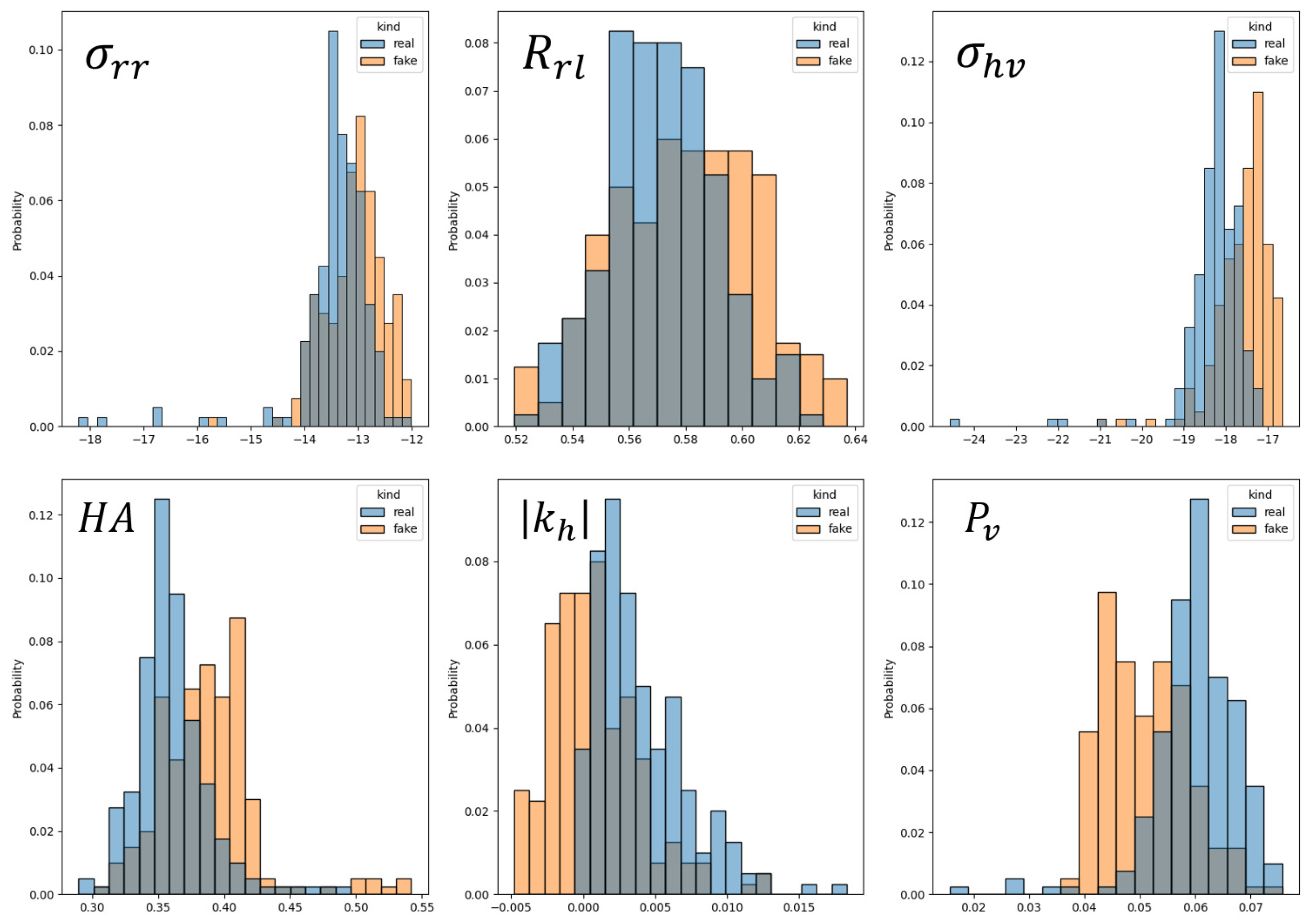
Figure 7 and Figure 8 provide a detailed comparison of the feature distributions between the real and synthetic data generated by the CTGAN for the two minority classes. Figure 7 focuses on the peas class, showing the distributions for six exemplary features in the real data (blue columns) versus synthetic data (orange columns). Figure 8 repeats this comparison for those six features of the broadleaf class. In both figures, the synthetic data distributions generated by the CTGAN closely match those of the corresponding real data features. This consistency demonstrates the CTGAN’s ability to accurately model the underlying distributions existing in the real data. Notably, the CTGAN is also capable of reconstructing synthetic data in a wider range compared to real features. For instance the distribution of, some synthetic features in Figure 7 and Figure 8 extends beyond the maximum and minimum values of the real data. This extension reduces the risk of overfitting during the subsequent classifier training, as the models are exposed to a more diverse representation of each feature data during training. Overall, these distribution comparisons provide strong evidence that the CTGAN can successfully capture the statistical properties of the real data, thereby being able to generate synthetic data that are representative of the original samples. This fidelity facilitates the effective application of synthetic data for classification tasks.
5. Conclusions
This article investigated the performance of the CTGAN model for generating synthetic data, to reduce the impact of insufficient samples in crop classification. To study this issue, the features extracted from the optical and SAR images obtained from the RapidEye and UASAR sensors were employed. In this research, by using three classifiers, XGBoost, RF, and KNN, the quality of synthetic data generated by the CTGAN (as a state-of-the-art method) was evaluated in comparison to RUS, ROS, and SMOTE. In general, the results of this research demonstrated the significant superiority of the CTGAN over the comparative algorithms. While SMOTE generated synthetic data without considering the distribution of the real data, the CTGAN method took account of the data distribution during data generation. Furthermore, RUS and ROS did not generate desirable data that considerably improved the performance of classifiers compared to the CTGAN model. Furthermore, the quality of the synthetic data generated by the CTGAN was evaluated by comparing it to real data using statistical metrics. Specifically, the mean, standard deviation, and distributions of the different features were measured and compared. The results showed that the data produced by the CTGAN exhibited similarities to the real data across the aforementioned statistical metrics. This indicates that the synthetic data generated by the CTGAN accurately reflects the real data distribution. Therefore, the CTGAN network is a better alternative to the basic methods of generating synthetic datasets. However, it is important to acknowledge that using the CTGAN for synthetic data generation has certain limitations. One such limitation is the requirement of a minimum amount of data for training. The CTGAN relies on a sufficient quantity of training data to effectively learn the underlying data distribution and capture the intricate dependencies within the dataset. Additionally, it is worth noting that the training process of the CTGAN can be more time-consuming compared to the traditional data generation methods. The CTGAN involves training a generative model that learns the complex patterns and relationships inherent in the data. This training process typically requires multiple iterations and can be computationally intensive, especially when dealing with large and high-dimensional datasets. The processing time required for training the CTGAN should be considered when deciding on an appropriate data generation approach, especially in time-sensitive applications or scenarios with resource constraints. Despite these limitations, the benefits of the CTGAN should not be overlooked. The CTGAN excels at capturing the underlying data distribution and generating synthetic samples that closely resemble the real data. It has the potential to overcome the limitations of traditional methods by preserving complex relationships and dependencies present in the original dataset. Additionally, the CTGAN offers more flexibility in generating synthetic data with the desired characteristics, allowing researchers to control specific features or adjust the balance between classes.
Some important directions for future work include the following: (1) Applying the CTGAN and comparing its performance to other generative models in other remote sensing applications, beyond crop classification. This could include tasks like land cover mapping, object detection in aerial/satellite imagery, and environmental monitoring. Evaluating generative solutions across different problem types would expand our understanding of their capabilities and limitations. (2) Leveraging synthetic data generation to address the lack of training samples in various remote sensing and geospatial problems beyond agriculture, such as damage assessment from natural disasters, urban development monitoring, infrastructure mapping, and species habitat modeling; where limited labeled data exist, generative models may help boost predictive accuracy. (3) Developing new generative model architectures and training procedures specialized for different remote sensing inputs.
Author Contributions
Ali Mirzaei: Methodology, statistical analysis, data analysis, figure preparation, and writing of the original draft. Hossein Bagheri: Conceptualization, supervision of the project, guidance in data analysis, literature review, methodology, critical revision of the manuscript, data analysis, writing, and experimental design. Iman Khosravi: Data collection, writting, and literature review. All authors have read and agreed to the published version of the manuscript.
Funding
This research received no external funding.
Data Availability Statement
The data presented in this study are available on request from the corresponding author.
Acknowledgments
The authors would like to present their acknowledgments to the JPL NASA, MacDonald, Dettwiler and Associates Ltd., the German Aerospace Center (DLR) DLR, the SMAPVEX 2012 team, the Agriculture and Agri-Food Canada, and Saeid Homayouni, from the Dept. of Geography, Environment, and Geomatics of the University of Ottawa, Canada, for providing the PolSAR and the fields survey data used in this research.
Conflicts of Interest
The authors declare no conflict of interest.
References
- Siachalou, S.; Mallinis, G.; Tsakiri-Strati, M. A hidden Markov models approach for crop classification: Linking crop phenology to time series of multi-sensor remote sensing data. Remote Sens. 2015, 7, 3633–3650. [Google Scholar] [CrossRef]
- Kross, A.; McNairn, H.; Lapen, D.; Sunohara, M.; Champagne, C. Assessment of RapidEye vegetation indices for estimation of leaf area index and biomass in corn and soybean crops. Int. J. Appl. Earth Obs. Geoinf. 2015, 34, 235–248. [Google Scholar] [CrossRef]
- Niazmardi, S.; Homayouni, S.; Safari, A. A computationally efficient multi-domain active learning method for crop mapping using satellite image time-series. Int. J. Remote Sens. 2019, 40, 6383–6394. [Google Scholar] [CrossRef]
- Niazmardi, S.; Homayouni, S.; Safari, A.; Shang, J.; McNairn, H. Multiple kernel representation and classification of multivariate satellite-image time-series for crop mapping. Int. J. Remote Sens. 2018, 39, 149–168. [Google Scholar] [CrossRef]
- Saini, R. Integrating Vegetation Indices and Spectral Features for Vegetation Mapping from Multispectral Satellite Imagery Using AdaBoost and Random Forest Machine Learning Classifiers. Geomat. Environ. Eng. 2023, 17, 57–74. [Google Scholar] [CrossRef]
- Hamidi, M.; Safari, A.; Homayouni, S. An auto-encoder based classifier for crop mapping from multitemporal multispectral imagery. Int. J. Remote Sens. 2021, 42, 986–1016. [Google Scholar] [CrossRef]
- Hosseini, M.; McNairn, H.; Merzouki, A.; Pacheco, A. Estimation of Leaf Area Index (LAI) in corn and soybeans using multi-polarization C-band L-band radar data. Remote Sens. Environ. 2015, 170, 77–89. [Google Scholar] [CrossRef]
- Sultana, S.; Arima, E.Y.; Tasker, K.A. Combining H/A/Alpha polarimetric decomposition of PolSAR data with image classification for wetland identification: A case study of Pacaya-Samiria National Reserve, Peru. Pap. Appl. Geogr. 2016, 2, 9–24. [Google Scholar] [CrossRef]
- Khosravi, I.; Safari, A.; Homayouni, S.; McNairn, H. Enhanced decision tree ensembles for land-cover mapping from fully polarimetric SAR data. Int. J. Remote Sens. 2017, 38, 7138–7160. [Google Scholar] [CrossRef]
- Tamiminia, H.; Homayouni, S.; McNairn, H.; Safari, A. A particle swarm optimized kernel-based clustering method for crop mapping from multi-temporal polarimetric L-band SAR observations. Int. J. Appl. Earth Obs. Geoinf. 2017, 58, 201–212. [Google Scholar] [CrossRef]
- Whelen, T.; Siqueira, P. Use of time-series L-band UAVSAR data for the classification of agricultural fields in the San Joaquin Valley. Remote Sens. Environ. 2017, 193, 216–224. [Google Scholar] [CrossRef]
- Reisi-Gahrouei, O.; Homayouni, S.; McNairn, H.; Hosseini, M.; Safari, A. Crop biomass estimation using multi regression analysis and neural networks from multitemporal L-band polarimetric synthetic aperture radar data. Int. J. Remote Sens. 2019, 40, 6822–6840. [Google Scholar] [CrossRef]
- Khosravi, I.; Razoumny, Y.; Hatami Afkoueieh, J.; Alavipanah, S.K. Fully polarimetric synthetic aperture radar data classification using probabilistic and non-probabilistic kernel methods. Eur. J. Remote Sens. 2021, 54, 310–317. [Google Scholar] [CrossRef]
- Khosravi, I.; Safari, A.; Homayouni, S. MSMD: Maximum separability and minimum dependency feature selection for cropland classification from optical and radar data. Int. J. Remote Sens. 2018, 39, 2159–2176. [Google Scholar] [CrossRef]
- Khosravi, I.; Alavipanah, S.K. A random forest-based framework for crop mapping using temporal, spectral, textural and polarimetric observations. Int. J. Remote Sens. 2019, 40, 7221–7251. [Google Scholar] [CrossRef]
- Khosravi, I.; Razoumny, Y.; Hatami Afkoueieh, J.; Alavipanah, S.K. An ensemble method based on rotation calibrated least squares support vector machine for multi-source data classification. Int. J. Image Data Fusion 2021, 12, 48–63. [Google Scholar] [CrossRef]
- Ustuner, M.; Sanli, F.; Abdikan, S. Balanced vs imbalanced training data: Classifying RapidEye data with support vector machines. Int. Arch. Photogramm. Remote Sens. Spat. Inf. Sci. 2016, 41, 379–384. [Google Scholar] [CrossRef]
- Longadge, R.; Dongre, S. Class imbalance problem in data mining review. Indones. J. Electr. Eng. Comput. Sci. 2013. [Google Scholar] [CrossRef]
- Cenggoro, T.W.; Isa, S.M.; Kusuma, G.P.; Pardamean, B. Classification of imbalanced land-use/land-cover data using variational semi-supervised learning. In Proceedings of the 2017 International Conference on Innovative and Creative Information Technology (ICITech), Salatiga, Indonesia, 2–4 November 2017; pp. 1–6. [Google Scholar]
- Johnson, B.A.; Iizuka, K. Integrating OpenStreetMap crowdsourced data and Landsat time-series imagery for rapid land use/land cover (LULC) mapping: Case study of the Laguna de Bay area of the Philippines. Appl. Geogr. 2016, 67, 140–149. [Google Scholar] [CrossRef]
- Bogner, C.; Seo, B.; Rohner, D.; Reineking, B. Classification of rare land cover types: Distinguishing annual and perennial crops in an agricultural catchment in South Korea. PLoS ONE 2018, 13, e0190476. [Google Scholar] [CrossRef]
- Douzas, G.; Bacao, F.; Fonseca, J.; Khudinyan, M. Imbalanced learning in land cover classification: Improving minority classes’ prediction accuracy using the geometric SMOTE algorithm. Remote Sens. 2019, 11, 3040. [Google Scholar] [CrossRef]
- Fonseca, J.; Douzas, G.; Bacao, F. Improving imbalanced and cover classification with K-Means SMOTE: Detecting and oversampling distinctive minority spectral signatures. Information 2021, 12, 266. [Google Scholar] [CrossRef]
- Fonseca, J.; Douzas, G.; Bacao, F. Increasing the Effectiveness of Active Learning: Introducing Artificial Data Generation in Active Learning for Land Use/Land Cover Classification. Remote Sens. 2021, 13, 2619. [Google Scholar] [CrossRef]
- Hai Ly, N.; Nguyen, H.D.; Loubiere, P.; Van Tran, T.; Șerban, G.; Zelenakova, M.; Brețcan, P.; Laffly, D. The composition of time-series images and using the technique SMOTE ENN for balancing datasets in land use/cover mapping. Acta Montan Slovaca 2022, 27, 342–359. [Google Scholar]
- Ebrahimy, H.; Mirbagheri, B.; Matkan, A.A.; Azadbakht, M. Effectiveness of the integration of data balancing techniques and tree-based ensemble machine learning algorithms for spatially-explicit land cover accuracy prediction. Remote Sens. Appl. Soc. Environ. 2022, 27, 100785. [Google Scholar] [CrossRef]
- Goodfellow, I.; Pouget-Abadie, J.; Mirza, M.; Xu, B.; Warde-Farley, D.; Ozair, S.; Courville, A.; Bengio, Y. Generative Adversarial Nets in Advances in Neural Information Processing Systems (NIPS); Curran Associates, Inc.: Red Hook, NY, USA, 2014; pp. 2672–2680. [Google Scholar]
- Xu, L.; Skoularidou, M.; Cuesta-Infante, A.; Veeramachaneni, K. Modeling tabular data using conditional GAN. In Proceedings of the Advances in Neural Information Processing Systems 32 (NeurIPS 2019), Vancouver, BC, Canada, 8–14 December 2019. [Google Scholar]
- McNairn, H.; Jackson, T.J.; Wiseman, G.; Belair, S.; Berg, A.; Bullock, P.; Colliander, A.; Cosh, M.H.; Kim, S.B.; Magagi, R. The soil moisture active passive validation experiment 2012 (SMAPVEX12): Prelaunch calibration and validation of the SMAP soil moisture algorithms. IEEE Trans. Geosci. Remote Sens. 2014, 53, 2784–2801. [Google Scholar] [CrossRef]
- Bagheri, H.; Schmitt, M.; d’Angelo, P.; Zhu, X.X. A framework for SAR-optical stereogrammetry over urban areas. ISPRS J. Photogramm. Remote Sens. 2018, 146, 389–408. [Google Scholar] [CrossRef]
- Peña-Barragán, J.M.; Ngugi, M.K.; Plant, R.E.; Six, J. Object-based crop identification using multiple vegetation indices, textural features and crop phenology. Remote Sens. Environ. 2011, 115, 1301–1316. [Google Scholar] [CrossRef]
- Hoang, H.K.; Bernier, M.; Duchesne, S.; Tran, Y.M. Rice mapping using RADARSAT-2 dual-and quad-pol data in a complex land-use Watershed: Cau River Basin (Vietnam). IEEE J. Sel. Top. Appl. Earth Obs. Remote Sens. 2016, 9, 3082–3096. [Google Scholar] [CrossRef]
- Belgiu, M.; Drăguţ, L. Random forest in remote sensing: A review of applications and future directions. ISPRS J. Photogramm. Remote Sens. 2016, 114, 24–31. [Google Scholar] [CrossRef]
- Mhanna, S.; Halloran, L.J.; Zwahlen, F.; Asaad, A.H.; Brunner, P. Using machine learning and remote sensing to track land use/land cover changes due to armed conflict. Sci. Total. Environ. 2023, 898, 165600. [Google Scholar] [CrossRef] [PubMed]
- Zhu, X.X.; Hu, J.; Qiu, C.; Shi, Y.; Kang, J.; Mou, L.; Bagheri, H.; Haberle, M.; Hua, Y.; Huang, R. So2Sat LCZ42: A benchmark dataset for the classification of global local climate zones [Software and Data Sets]. IEEE Geosci. Remote Sens. Mag. 2020, 8, 76–89. [Google Scholar] [CrossRef]
- Kafy, A.A.; Saha, M.; Rahaman, Z.A.; Rahman, M.T.; Liu, D.; Fattah, M.A.; Al Rakib, A.; AlDousari, A.E.; Rahaman, S.N.; Hasan, M.Z. Predicting the impacts of land use/land cover changes on seasonal urban thermal characteristics using machine learning algorithms. Build. Environ. 2022, 217, 109066. [Google Scholar] [CrossRef]
- Mountrakis, G.; Im, J.; Ogole, C. Support vector machines in remote sensing: A review. ISPRS J. Photogramm. Remote Sens. 2011, 66, 247–259. [Google Scholar] [CrossRef]
- He, Y.; Lee, E.; Warner, T.A. A time series of annual land use and land cover maps of China from 1982 to 2013 generated using AVHRR GIMMS NDVI3g data. Remote Sens. Environ. 2017, 199, 201–217. [Google Scholar] [CrossRef]
- Chan, J.C.W.; Paelinckx, D. Evaluation of Random Forest and Adaboost tree-based ensemble classification and spectral band selection for ecotope mapping using airborne hyperspectral imagery. Remote Sens. Environ. 2008, 112, 2999–3011. [Google Scholar] [CrossRef]
- Maselli, F.; Chirici, G.; Bottai, L.; Corona, P.; Marchetti, M. Estimation of Mediterranean forest attributes by the application of k-NN procedures to multitemporal Landsat ETM+ images. Int. J. Remote Sens. 2005, 26, 3781–3796. [Google Scholar] [CrossRef]
- Chawla, N.V.; Japkowicz, N.; Kotcz, A. Special issue on learning from imbalanced data sets. ACM SIGKDD Explor. Newsl. 2004, 6, 1–6. [Google Scholar] [CrossRef]
- Alem, A.; Kumar, S. Deep learning methods for land cover and land use classification in remote sensing: A review. In Proceedings of the 2020 8th International Conference on Reliability, Infocom Technologies and Optimization (Trends and Future Directions) (ICRITO), Noida, India, 4–5 June 2020; pp. 903–908. [Google Scholar]
- Moon, J.; Jung, S.; Park, S.; Hwang, E. Conditional tabular GAN-based two-stage data generation scheme for short-term load forecasting. IEEE Access 2020, 8, 205327–205339. [Google Scholar] [CrossRef]
- Lee, J.; Lee, O. CTGAN vs TGAN? which one is more suitable for generating synthetic eeg data. J. Theor. Appl. Inf. Technol. 2021, 99, 2359–2372. [Google Scholar]
- Habibi, O.; Chemmakha, M.; Lazaar, M. Imbalanced tabular data modelization using CTGAN and machine learning to improve IoT Botnet attacks detection. Eng. Appl. Artif. Intell. 2023, 118, 105669. [Google Scholar] [CrossRef]
- Akosa, J. Predictive accuracy: A misleading performance measure for highly imbalanced data. In Proceedings of the SAS Global Forum, Orlando, FL, USA, 2–5 April 2017; Volume 12, pp. 1–4. [Google Scholar]
Figure 1.
The study area and the reference data in this research.

Figure 2.
The framework implemented for synthetic data generation and cropland classification.

Figure 3.
The structure of CTGAN for synthetic data generation.

Figure 4.
Confusion matrices for the RF classifier trained and tested on (a) original, (b) RUS, (c) ROS, (d) SMOTE (e) and CTGAN datasets.
Figure 4.
Confusion matrices for the RF classifier trained and tested on (a) original, (b) RUS, (c) ROS, (d) SMOTE (e) and CTGAN datasets.

Figure 5.
Performance of the KNN classifier, measured using the F1 score metric, in relation to varying quantities of synthetic samples generated with the CTGAN model.
Figure 5.
Performance of the KNN classifier, measured using the F1 score metric, in relation to varying quantities of synthetic samples generated with the CTGAN model.

Figure 6.
Correlation plots between the means and standard deviations of synthetic data and real data. Each blue point corresponds to a feature extracted from SAR and optical images.
Figure 6.
Correlation plots between the means and standard deviations of synthetic data and real data. Each blue point corresponds to a feature extracted from SAR and optical images.

Figure 7.
The data distribution of six exemplary features generated using the CTGAN versus the distribution of the real data for the peas class (The blue histogram represents the distribution of real data, the orange histogram depicts the distribution of fake data, and the gray columns illustrate the overlap of the distributions of real and fake data).

Figure 8.
The data distribution of six exemplary features generated using the CTGAN versus the distribution of the real data for the broadleaf class (The blue histogram represents the distribution of real data, the orange histogram depicts the distribution of fake data, and the gray columns illustrate the overlap of the distributions of real and fake data).


Table 1.
Preview of previous studies that used data generation methods to improve the accuracy of classification.
Table 1.
Preview of previous studies that used data generation methods to improve the accuracy of classification.
| Author | Sensor | Study Area | Data Generation Method |
|---|---|---|---|
| Sani et al., 2017 [19] | Landsat 7 | Jakarta City | Variational semi-supervised learning |
| Douzas et al., 2019 [22] | Landsat 8 | North-western Portugal | SMOTE |
| Fonseca et al., 2021 [23] | Hyperion, AVIRIS, ROSIS | Okavango Delta, Botswana, Pavia, northern Italy, Kennedy Space Center, Florida, Salinas Valley, North-western Indiana | SMOTE |
| Fonseca et al., 2021 [24] | Hyperion, AVIRIS, ROSIS | Okavango Delta, Botswana, Pavia, northern Italy, Kennedy Space Center, Florida, Salinas Valley, North-western Indiana | SMOTE |
| Hai Ly et al., 2022 [25] | Landsat 8 | Central region of Vietnam | SMOTE |
| Hamid Ebrahimy et al., 2022 [26] | Sentinel 2 | Different parts of Iran | ROS, SMOTE, Adaptive synthetic sampling |
Table 2.
The ratio of the number of samples for each class to the number of samples for the majority class.
Table 2.
The ratio of the number of samples for each class to the number of samples for the majority class.
| Class | Original Dataset (IR%) | After Synthetic Data Generation (IR%) |
|---|---|---|
| Corn | 0.460 | 0.460 |
| Peas | 0.002 | 0.12 |
| Canola | 0.889 | 0.889 |
| Soybeans | 0.871 | 0.871 |
| Oats | 0.554 | 0.554 |
| Wheat | 1 | 1 |
| Broadleaf | 0.002 | 0.12 |
Table 3.
The features derived from optical imagery (RapidEye) used in this research.
| Name | Symbol |
|---|---|
| Spectral channels | B, G, R, RE, NIR |
| Vegetation indices | NDVI, SR, RGRI, EVI, ARVI, SAVI, NDGI, gNDVI, MTVI2, , , , , RNDVI, TCARI, TVI, PRI2 |
| Texture indicators | , , , , , , , , , , , , , , , |
Table 4.
The polarimetric features derived from SAR imagery (UAVSAR) used in this research.
| Name | Symbol |
|---|---|
| Backscattering intensities (dB) | , , , , , |
| Polarization ratio (dB) | , , , , , |
| Ratio values | , , , , , |
| PolSAR correlation coefficients | , , , , , |
| Cloud & Pottier parameters | H, A, , H(1–A), (1–H)A, (1–H)(1–A), , , and , , RVI |
| Pauli parameters | , |
| Krogager parameters | , |
| Freeman-Durden parameters | , , |
| Yamaguchi parameters | , , , |
Table 5.
The hyperparameters tuned for the different classifiers and synthetic data generators.
| Classifier or Data Generator | Hyperparameters |
|---|---|
| XGBoost | No. of estimators = 1000, max depth = 18, max features = 1, bootstrap = True, max samples = 0.9 |
| RF | No. of estimators = 1000, max depth = 18, max features = 0.6, bootstrap = True, max samples = 0.8 |
| KNN | No. of neighbors = 10, weights = distance, metric = Manhattan |
| CTGAN | layers = 2, neurons in each layer = 255, Optimizer = Adam, learning rate = 0.002, epoch = 300 |
| SMOTE | Sampling strategy = not majority, k neighbors = 5 |
Table 6.
The sensitivity of the different classifiers after data generation using various methods. The sensitivity was improved for all classifiers after generating data using the different methods.
Table 6.
The sensitivity of the different classifiers after data generation using various methods. The sensitivity was improved for all classifiers after generating data using the different methods.
| Classifier | XGBoost | RF | KNN | ||||||
|---|---|---|---|---|---|---|---|---|---|
| Data Set∖Class | Peas | Broadleaf | Total Sensitivity | Peas | Broadleaf | Total Sensitivity | Peas | Broadleaf | Total Sensitivity |
| Original | 0.856 | 0.850 | 0.98 | 0.928 | 0.800 | 0.98 | 0.011 | 0.028 | 0.86 |
| RUS | 0.950 | 0.983 | 0.87 | 0.983 | 0.989 | 0.88 | 0.722 | 0.583 | 0.49 |
| ROS | 0.872 | 0.878 | 0.98 | 0.918 | 0.811 | 0.98 | 0.350 | 0.274 | 0.86 |
| SMOTE | 0.867 | 0.933 | 0.98 | 0.928 | 0.878 | 0.98 | 0.717 | 0.794 | 0.86 |
| CTGAN | 0.950 | 0.939 | 0.98 | 0.950 | 0.950 | 0.98 | 0.922 | 0.772 | 0.86 |
Table 7.
of XGBoost for the different crop classes.
| Class | Insufficient and Imbalance | RUS | ROS | SMOTE | CTGAN |
|---|---|---|---|---|---|
| Corn | 0.994 | 0.956 | 0.954 | 0.993 | 0.994 |
| Peas | 0.925 | 0.972 | 0.591 | 0.931 | 0.975 |
| Canola | 0.998 | 0.989 | 0.981 | 0.998 | 0.998 |
| Soybeans | 0.995 | 0.950 | 0.947 | 0.994 | 0.995 |
| Oats | 0.973 | 0.849 | 0.787 | 0.970 | 0.973 |
| Wheat | 0.986 | 0.848 | 0.865 | 0.985 | 0.986 |
| Broadleaf | 0.922 | 0.990 | 0.567 | 0.966 | 0.969 |
Disclaimer/Publisher’s Note: The statements, opinions and data contained in all publications are solely those of the individual author(s) and contributor(s) and not of MDPI and/or the editor(s). MDPI and/or the editor(s) disclaim responsibility for any injury to people or property resulting from any ideas, methods, instructions or products referred to in the content. |
© 2023 by the authors. Licensee MDPI, Basel, Switzerland. This article is an open access article distributed under the terms and conditions of the Creative Commons Attribution (CC BY) license (https://creativecommons.org/licenses/by/4.0/).
Share and Cite
MDPI and ACS Style
Mirzaei, A.; Bagheri, H.; Khosravi, I. Enhancing Crop Classification Accuracy through Synthetic SAR-Optical Data Generation Using Deep Learning. ISPRS Int. J. Geo-Inf. 2023, 12, 450. https://doi.org/10.3390/ijgi12110450
AMA Style
Mirzaei A, Bagheri H, Khosravi I. Enhancing Crop Classification Accuracy through Synthetic SAR-Optical Data Generation Using Deep Learning. ISPRS International Journal of Geo-Information. 2023; 12(11):450. https://doi.org/10.3390/ijgi12110450
Chicago/Turabian StyleMirzaei, Ali, Hossein Bagheri, and Iman Khosravi. 2023. "Enhancing Crop Classification Accuracy through Synthetic SAR-Optical Data Generation Using Deep Learning" ISPRS International Journal of Geo-Information 12, no. 11: 450. https://doi.org/10.3390/ijgi12110450
Note that from the first issue of 2016, this journal uses article numbers instead of page numbers. See further details here.