1. Introduction
Visual coverage is an essential quantifiable feature of an individual camera and camera network, which perform the most fundamental requirements of any surveillance tasks and computer vision applications. Such diverse applications as camera reconfiguration, optimal camera placement, camera selection, camera calibration, and tracking correspondence are required for capturing coverage information, even though they vary in objectives and constraints. Virtually all camera network applications depend on or can benefit from knowledge about the coverage of individual cameras, the coverage of the network as a whole, and the relationships of cameras in terms of their coverage [
1]. Camera coverage is always an essential issue in Visual Sensor Network (VSN), Directional Sensor Network (DSN), and Wireless Multimedia Sensor Network (WMSN). Visual coverage is also an important issue for (geo-tagged) video data models and retrieval [
2], video geospatial analysis [
3] and the integration of GIS and video surveillance [
4,
5,
6].
In the surveillance system, the physical coverage is crucial for spatial analysis, for example to determine whether a suspect or vehicle is exactly covered by a certain camera, to count the number of a certain kind of features covered by camera network, and so on. Consequently, the accurate geometry of the individual cameras and camera network is desperately needed. Moreover, the acceptable speed for coverage estimation is crucial when the number of cameras is large or/and the parameters will be changed frequently—for example optimal camera network deployment, camera network reconfiguration, and so on. Consequently, coverage estimation method considering the trade-off of efficacy and accuracy is desirable.
References are seldom explicit concerning the process of estimating coverage even though almost all applications aim to maximize the overall coverage area sometimes with other constraints, which depend upon the specific application. The coverage problem involves camera parameters, a scene model and task parameters [
1]. Because the works themselves are very complex and time-consuming, requiring some approximations when dealing with coverage, the camera model and scene model are often simplified according to the task. The camera model is simplified as a fixed-size sector or quadrilateral. The target fields are often considered as a 2D plane with or without obstacles. A few references investigate algorithms for applications such as coverage optimization considering 3D modeling of the monitored area. In experimental applications, the target area is sampled by regularly arranged grids, so the overall coverage of the target area is represented by the coverage of these grids [
7]. It is less time-consuming than methods without sampling, but the result is that simulated experiments with the above assumptions are discordant with the actual applications. These works emphasize efficacy rather than accuracy, and the geometry of the individual cameras and camera network is ignored.
In this paper, we estimate camera coverage considering the trade-off of efficacy and accuracy. We propose a grid subdivision algorithm for estimating camera coverage. The main idea is that the surveillance area is divided gradually into grids of multiple grid sizes, while the coverage area depends on the coverage statuses of grids in different subdivision levels for the following reasons: (1) the camera coverage is not large, which demands a high precision data source; (2) a high precision DEM (Digital Elevation Model) is not always accessible; and (3) the occlusions for line of sight (LOS) from cameras to targets, including buildings, vegetation and other surveyed heights, are often stored in vector features. We assume that the cameras are deployed in 3D geographic space while the surveillance area is a relatively flat ground plane with some occlusions such as buildings, trees and others in vector format. It is more suitable for real-world implementations in most city areas where the ground is seldom rolling.
The remainder of the paper is organized as follows. After a literature review of related work in the next section, the method is described in detail in the third section. Performance of the proposed method is validated through experiments with simulated data and cameras deployed in a real geographic space, and the results are evaluated in the fourth section. Finally, concluding remarks and discussions are presented.
2. Related Works
The researchers in VSN, DSN and WMSN often try to find an efficient algorithm to obtain an optimized configuration scheme for a camera network for different tasks, such as optimal placement [
7,
8], automated layout [
9], coverage-enhancement [
10,
11,
12,
13], coverage improvement [
14], planning optimization [
15,
16], coverage estimation [
17,
18], optimal deployment [
19,
20,
21], camera reconfiguration [
22], object coverage [
23], scalable target coverage [
24], resource-aware coverage [
25], etc. Hundreds of cameras are engaged and their parameters frequently changed to estimate coverage in real time, which poses substantial computational challenges. Thus, more emphasis is placed on specific camera coverage models for tasks than the optimization algorithms themselves.
The works mentioned above consider the 3D camera model, but the region of interest is simplified as a 2D plane with/without occlusions and sampled by grid points or control points. Even though this is a feasible way to estimate coverage rate and reduce computing time, it results in inaccurate estimation of the geometric shape of a camera or camera network. Ignorance of the coverage geometry cannot benefit camera network visualization, camera spatial retrieval or later spatial analysis.
Camera coverage can be considered as a particular viewshed analysis because it involves not only geographic data but also the imaging principle of cameras. Viewshed analysis is applied more frequently because of the many potential algorithm parameter changes such as altitude offset of the viewpoint, visible radius, location of viewpoints, effect of vegetation, light refraction, and curvature of the earth. The computational bottleneck poses a significant challenge to current GIS systems [
26]. Consequently, the classic viewshed algorithms, such as inter-visibility based on LOS, the Xdraw algorithm, and the reference plane algorithm were improved by a variety of algorithms to speed up calculations [
27,
28,
29,
30,
31]. Some authors proposed effective parallel viewshed algorithms [
26,
30,
32]. Current research mainly focuses on viewshed analysis in terrain models whose data structure is a DEM or TIN (Triangulated Irregular Network). When combined with a Digital Surface Model (or a Digital Terrain Model), the line of sight method is very effective for surveillance camera placement because it allows introduction of some important characteristics of cameras such as the 3D position of each camera, observation azimuth, field of view, the range of the camera, etc. [
33]. However, for most public sources of elevation data, the quality is variable and, in some areas, is very poor (especially in some mountain and desert void areas). This implies that in some situations it is difficult to obtain enough elevation points of the region of interest to build a proper DEM [
34]. Occlusions including buildings, vegetation and other surveyed heights are often stored in vector features. Argany et al. [
35] stated that besides positional accuracy, semantic accuracy, the completeness of spatial information, and the type of spatial representation of the real world is another important issue that has a significant impact on sensor network optimization. An accurate determination of sensor positions in a raster representation of the space such as in 3D city models is more difficult because visibility could be estimated more accurately in vector data [
35].
Overall, in VSN, DSN and WMSN, the researchers designed a camera coverage model to meet the demands of specific optimal tasks. Some of them employed 2D camera models with or without occlusions, and some of them presented 3D camera coverage models considering one or more of FOV (Field of View), resolution, focus, angle and occlusions. The criterion to estimate the camera network is the coverage rate that is determined by the coverage of grid points or control points sampled from the region of interest rather than the physical coverage of cameras. In GIS, the researchers implemented various effective viewshed analysis algorithms. In some works, camera coverage is estimated using an ArcGIS tool [
36]. However, the estimated coverage does not exactly conform to the projection principles of camera. An accurate and effective method to estimate camera coverage is desirable to visualize a camera’s physical FOV and various optimal applications of a camera network.
3. Camera Coverage Estimation
3.1. Overview of the Method
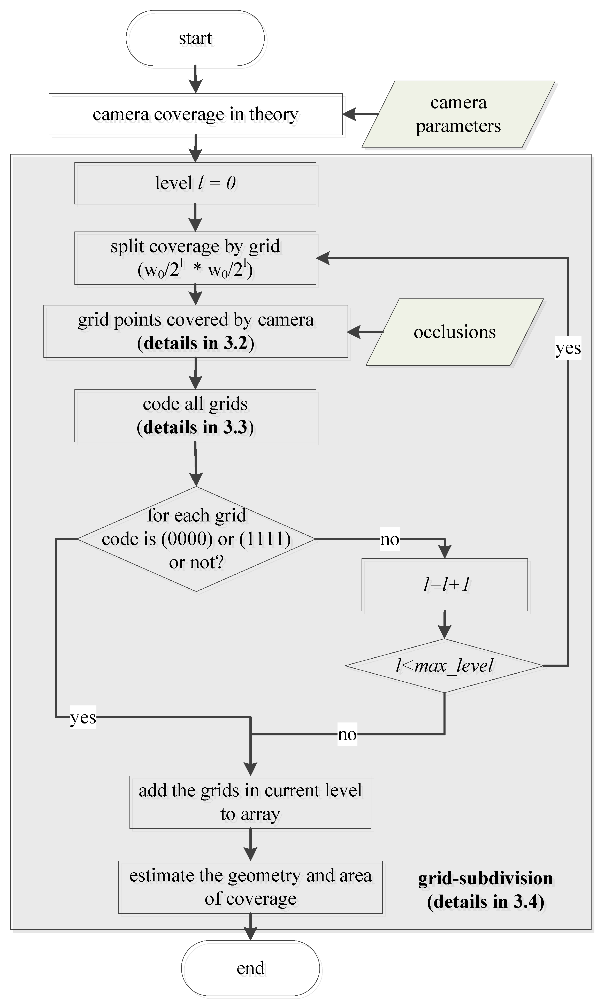
When the target area is sampled into regularly arranged grids of the same size, the grid size is the most important factor for coverage estimation [
35]. If it is undersized, the coverage estimation is of high precision and lower computing efficiency. If it is oversized, the coverage estimation is of low precision and higher computing efficiency because some details are ignored. It is hard to balance the precision and computing efficiency when the target area is sampled into grids of the same size. This paper proposes a method to meet this challenge. The proposed method is shown as
Figure 1.
First, the theoretical camera coverage and its minimum bounding rectangle (MBR) are computed according to camera parameters. Second, the minimum bounding rectangle is subdivided into grids of the initial size written as
, and the grid division level, which is written as
l, is set to 0. The status of each corner of a grid is estimated by the method depicted in
Section 3.2. If a corner point is covered by a camera, then its status is marked as ‘1’; otherwise, it is marked as ‘0’. Thus, four digital numbers (0 or 1) are used to code the status of a corresponding grid. Encoding (0000) means that the grid is not covered by a camera and encoding (1111) means that the entire grid is covered. Other encodings such as (0101), (0011), which contain both 0 and 1, mean that the grid is partly covered. The presentation status of a grid is discussed in
Section 3.3. Third, each grid in level
l whose encoding is not (0000) or (1111) must be subdivided into four sub-grids. The sub-grids will be divided until encoding is (0000) or (1111). Infinite subdivision is not appropriate because it is time-consuming and does not increase accuracy. We stop subdivision when the division level
l reaches the threshold
max_level. The detail of subdivision is presented in
Section 3.4. Finally, the geometry of camera coverage is the union of grids whose encoding is not (0000); the area is also estimated.
3.2. Coverage Model for Ground Point
Two conditions need to be satisfied if a point is covered by a camera: the ray from the camera to the point should intersect with the image plane and there should not be an obstacle between the camera and the point. The former relates to the camera model and the latter to obstacles in the geographic environment. The camera model is illustrated in
Figure 2. Camera
C is located at
. Its coverage in theory is the pyramid
C-D
1D
2D
3D
4, which is determined by intrinsic and external parameters of the camera. Intrinsic parameters include focal length
f, principle center (
u0,
v0), etc. External parameters include pan angle
P, tilt angle
T, roll angle
v, etc.
P is the angle between the north direction and the principal optic axis in a clockwise direction,
T is the angle from the horizontal direction to the principal optic axis in a clockwise direction, while
v is often close to 0 and is ignored in this paper. The point
G in the geographic environment is located at the coordinates (
XG,
YG,
HG), the corresponding image point
g, which is projected from point
G by a camera, is located at the coordinates (
x,
y) in an image coordinate system. The camera model is shown as Equation (1), where
λ is a non-zero scale factor:
A point
G is visible in an image if and only if the sight line
CG determined by camera
C and point
G crosses the image plane and there is no obstacle across the sight line
CG. As shown in
Figure 2, the point
G1 is visible, but the point
G2 is blocked by obstacle
B. The profile is shown in
Figure 3. (
XB,
YB,
HB) are the coordinates of
B. The height
H of the line of sight
CG at the location of
B is calculated by Equation (2):
where
. If
, then the current point is visible.
HB can be obtained from the attribute tables of vector data.
3.3. Presentation for Grid
Each grid has four corners, so its status can be represented by four digits (0 or 1) according to their visibility. We arranged them in the left-up corner followed by right-up, left-down, and right-down. Consequently, there are 16 possibilities, which are illustrated as
Table 1. If the status of the grid is (0000), the grid is not covered. If the status is (1111), the grid is covered. Other codes in the table represent partial coverages. As illustrated in
Table 1, the codes (0110) and (1001) lead to ambiguity. Under the circumstances, an extra point should be sampled in the grid center to confirm the actual coverage.
3.4. Multistage Grid Subdivision
After dividing the MBR into unified grids, each grid needs to be reviewed to determine whether it should be subdivided further according to its status as presented in
Section 3.3. For each grid in a level, there are two issues that need to be resolved: (a) convert and (b) conflict.
(a) convert
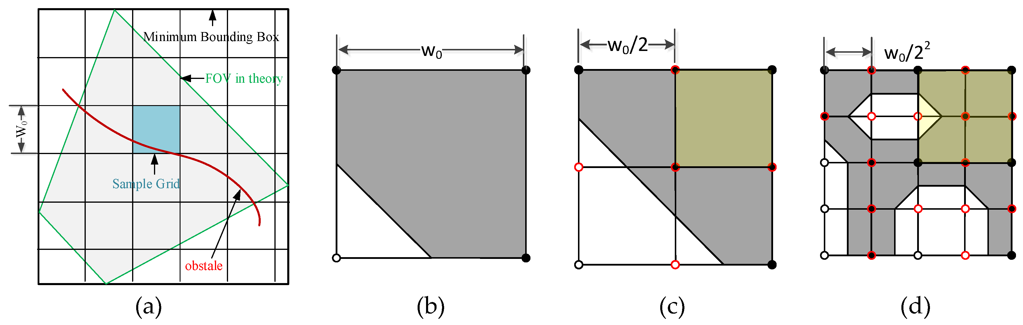
As shown in
Figure 4, the quadrilateral with the blue border is the FOV of the camera in theory. The rectangle with a black bold border is its MBR. The positions of left-down and right-up points of the MBR are (
XMin,
YMin) and (
XMax,
YMax). The MBR is divided into grids with the initial grid size
. We record a corner point as (
, where
l is the subdivision level of the points,
i and
j are the number of current corner points in the current subdivision level. A corner point (
and its location in geographic coordinate (
can be converted from one to the other by following Equations (3) and (4):
The points and are located at the same place. Likewise, the points and are the same point. When the grids are subdivided, only new points need to be estimated. Others can inherit their status from upper levels.
(b) conflict
The sample grid in blue shown in
Figure 4a, whose status is (1101) in level 0 (see
Figure 4b), is partly covered by the camera because of occlusion. Therefore, it needs further subdivision to the next level, which is shown in
Figure 4c. The right-up grid masked in yellow in
Figure 4c is coded as (1111); it does not need to be subdivided. However, its left neighbor grid needs to be subdivided, a new mid-point of the adjacent edge is added and its status is 0. This means that the grid masked in yellow must be subdivided because it is not completely covered by the camera. The current grid will be subdivided to the same level as its neighboring grid. Therefore, the grid is subdivided in
Figure 4d. Likewise, if the status of the new mid-point is 1 and its neighboring grid is coded as (0000), then the neighboring grid will be subdivided.
Here is the algorithm (Algorithm 1):
| Algorithms 1: Camera Coverage Estimation Based on Multistage Grid Subdivision |
| Input: Camera parameters, obstacle information, initial grid size w0, max level max_level |
| Output: Geometry and area of coverage |
| Process: |
| Subdivide the MBR of FOV in theory into grids with size w0 |
| Set current subdivision level l to 0. |
| While l < max_level and not all grids are coded as (0000) or (1111) do |
| l++ |
| for each grid in level l |
| Obtain and record the statuses of each grid (l, i, j). |
| If its code is not (0000) or (1111), then |
| detect the coverage statuses of five new points, which are composed of the center of the current grid, and the mid-points of four edges. |
| record the statuses of each grid. |
| For each new mid-point |
| if it conflicts with the neighbor grid, |
| then subdivide the neighbor grid to the current level.. |
| Convert the grid information from (l, i, j) to (X, Y) |
| Generate the geometry of coverage, which is the union of all the grids in different levels. |
| Obtain the area of coverage according to the geometry information. |
4. Experiments and Results
The initial grid size and max level are two important factors that affect the accuracy and efficiency of the proposed method. To determine the impacts of the initial size and level of grid on the proposed method, a series of experiments were performed using simulated and real data.
In the experiments, we used the number of points needing to be judged for coverage by the camera to represent the efficiency of the method because the judgment process is the most time-consuming step. The more points that need to be judged, the more time-consuming the process. We employed the percentage of coverage area relative to real area to represent the accuracy of the simulated experiments.
4.1. Prototype System
Our method is designed for camera coverage estimation for the prototype system shown in
Figure 5. The system is deployed in the sever with four main modules: (1) optimal camera network deployment, (2) camera control, (3) physical coverage visualization, and (4) spatial analysis for coverage. The system requires the accurate geometry of the individual cameras and camera network for coverage visualization and spatial analysis, and the acceptable speed to obtain optimal deployment scheme. Only the certain camera parameters need to be transferred between system and the corresponding camera other than camera coverage. The communication complexity is out of range of our method. Consequently, coverage estimation method considering the trade-off of efficacy and accuracy is desirable.
The experimental environment of this study is Ubuntu 64-bit operating system, Intel i5 processor, 2.0 G memory (San Jose, CA, USA, Apple). The study uses Python as the developing language, an open source QGIS to carry out geometric target description and topological relations operation.
4.2. Simulated Data
In this section, we employed three geometrical objects to simulate different geographic environments with different complexity. Three geometric shapes are covered by a camera, and the other areas covered by the camera are ignored because the process for them is the same for our method as for others. We employed a circle with a radius of 100 units, a diamond with side length of 100 units, and a five-pointed star with external and internal radiuses of 100 and 50 units to simulate different coverage situations. The circle is the simplest one, while the five-pointed star is the most complex.
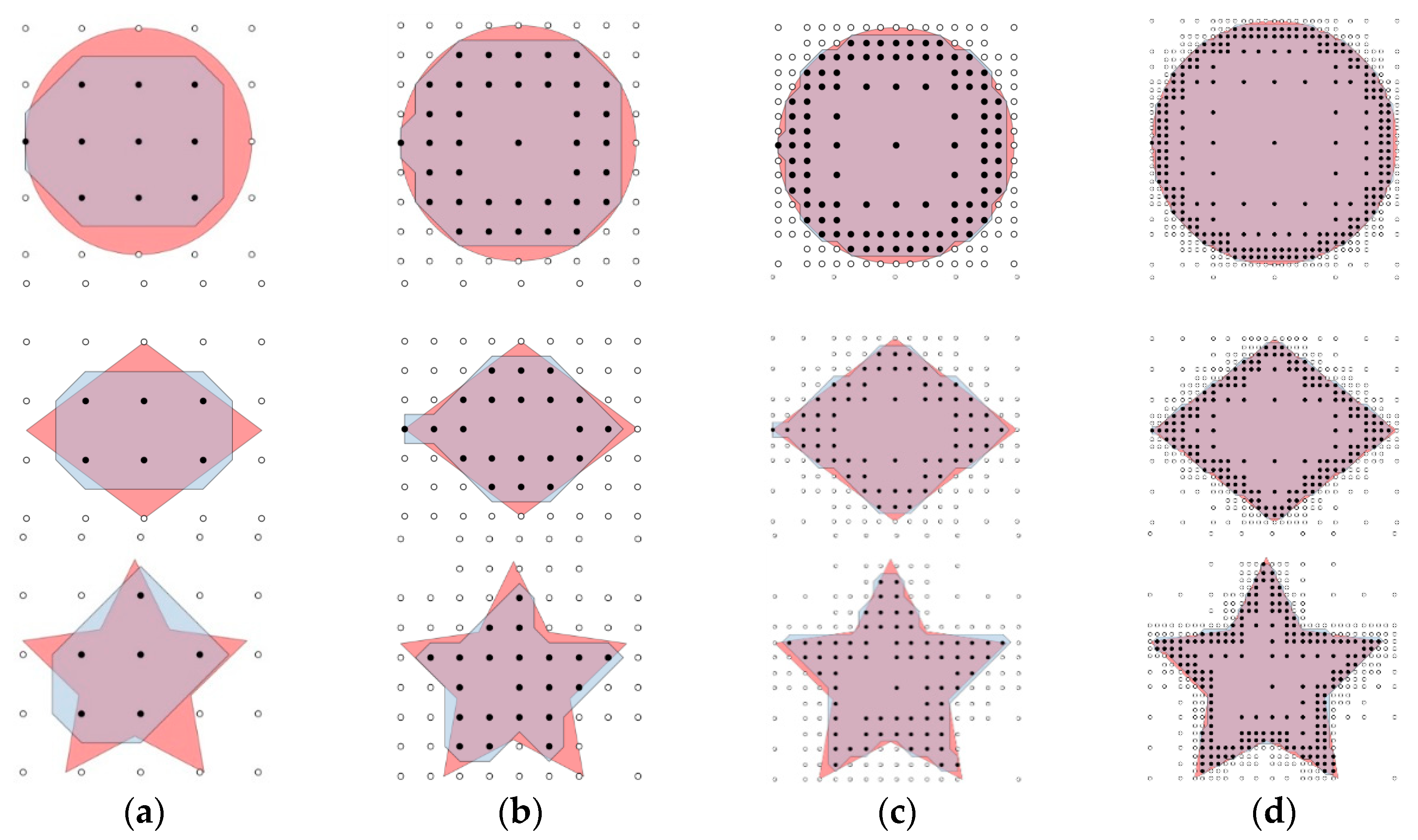
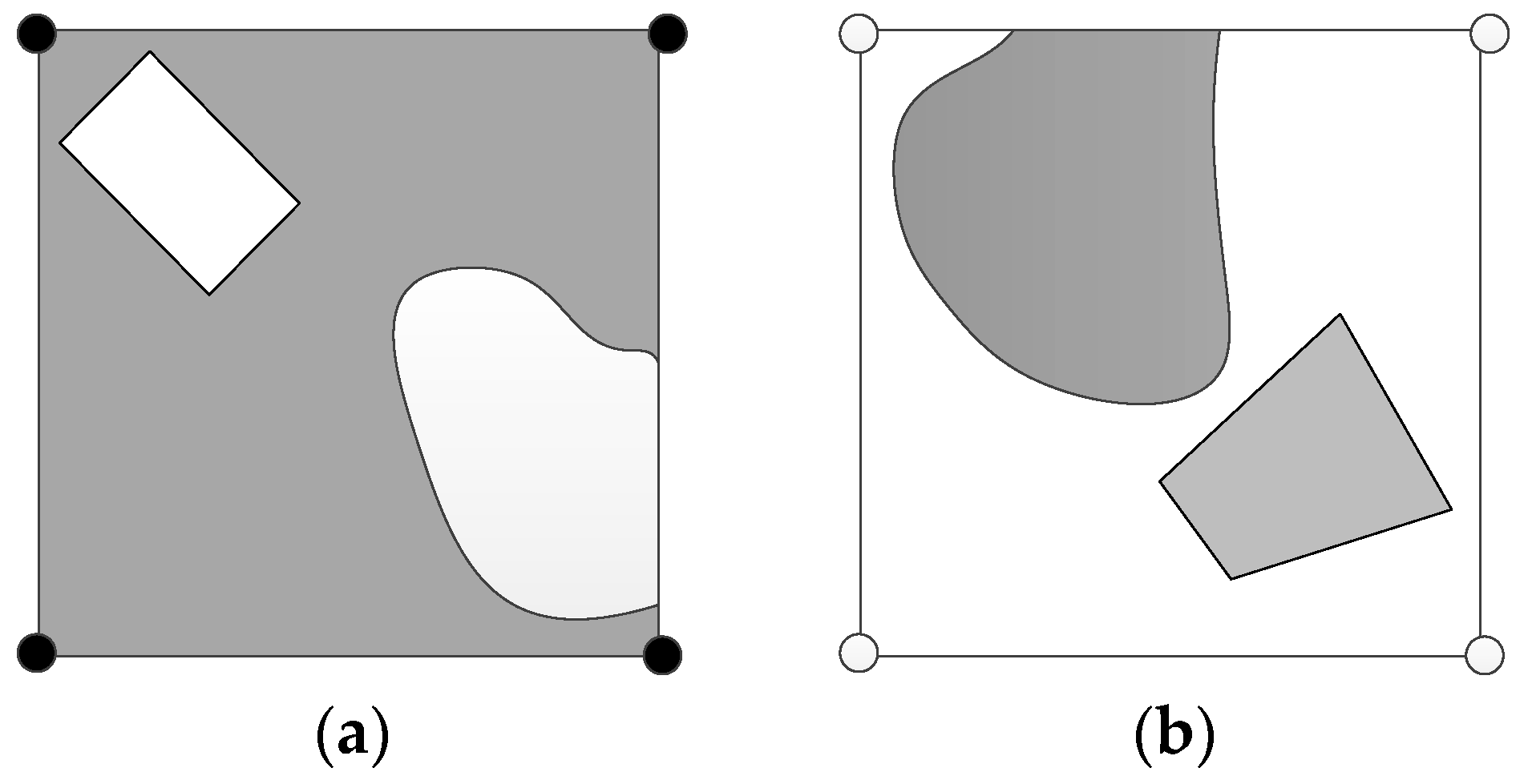
As shown in
Figure 6 and
Figure 7, the red area is the real coverage and the blue area is obtained by the proposed method with different initial grid sizes and max levels. Points filled with white mean the corner points are not covered by a camera while the ones filled with black mean that they are covered. In
Figure 6, the max level is set to 1, and the initial grid sizes are specified as 100, 75, 50, 25 and 5. Similarly, in
Figure 7, the initial grid sizes are set to 100, and the max level for subdivision is specified as 1, 2, 3 and 4.
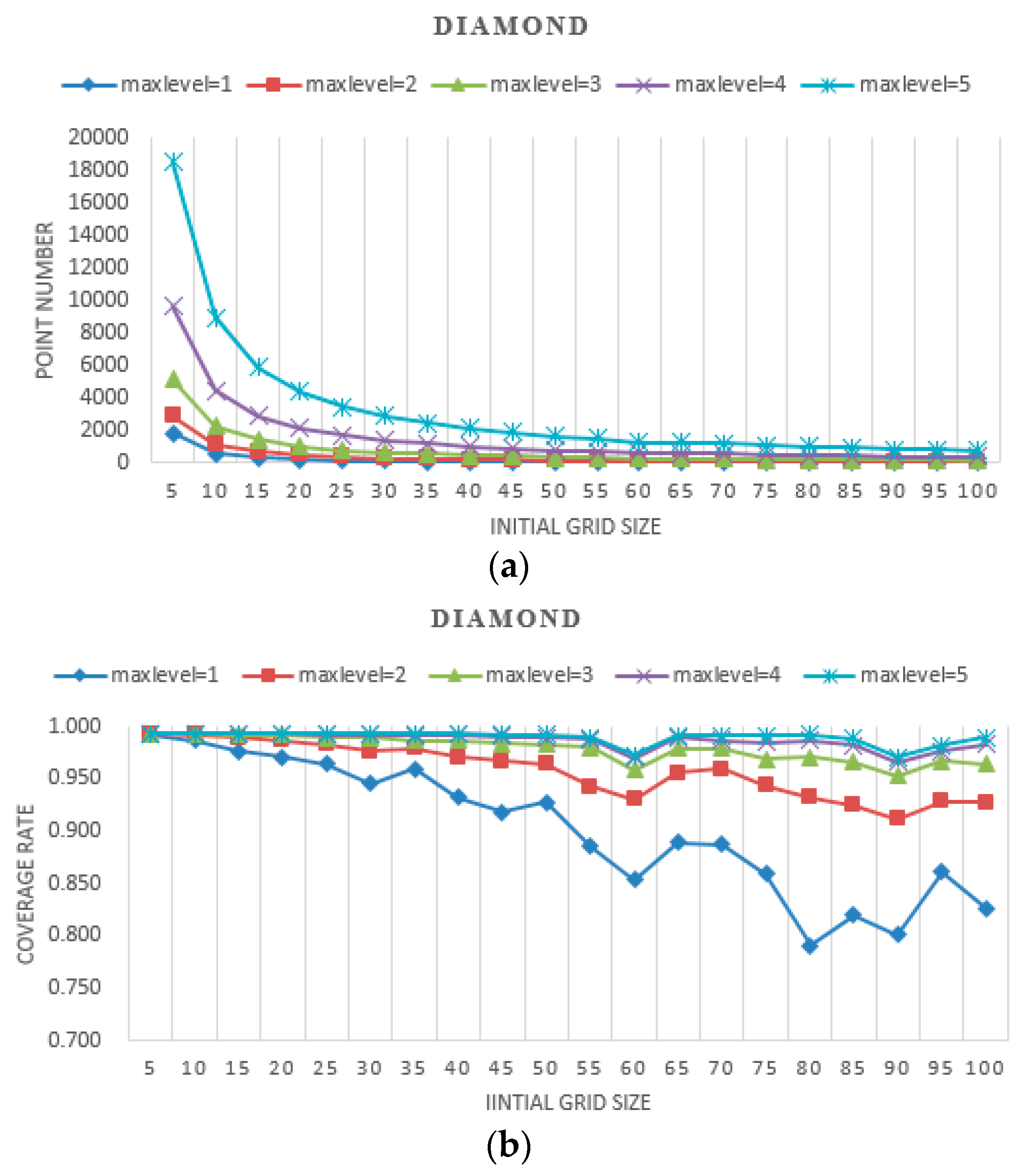
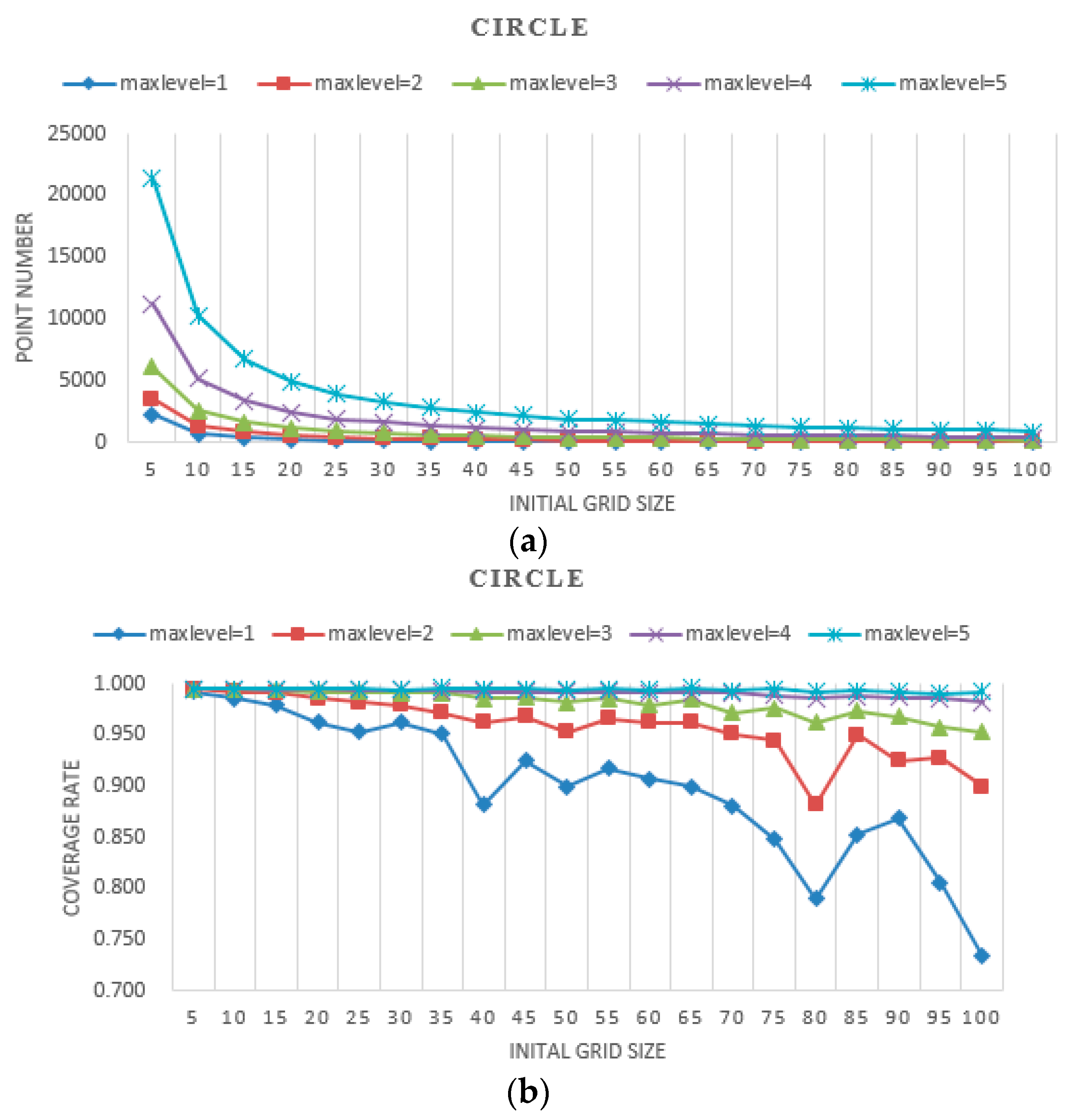
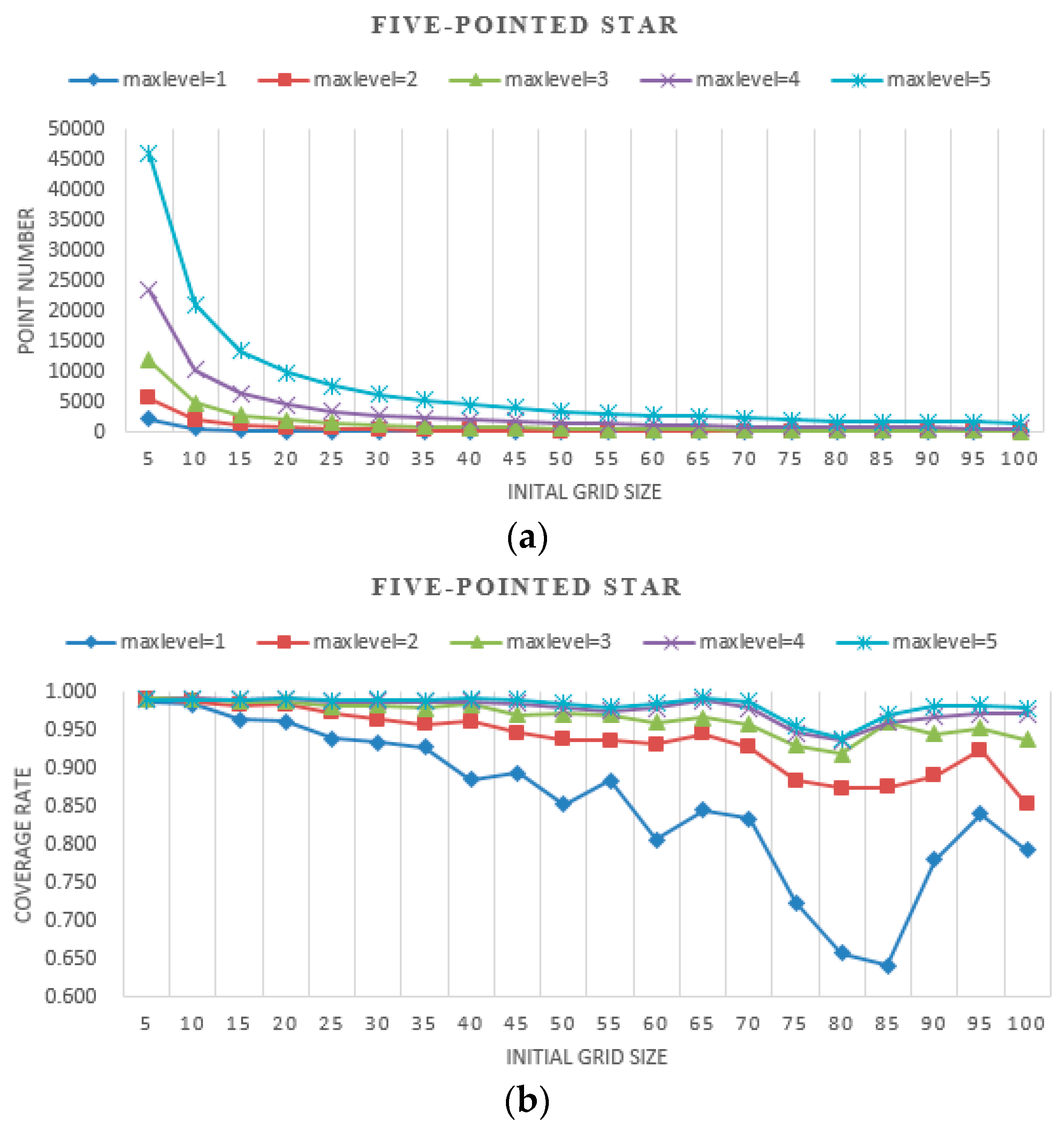
The results of experiments with different initial grid sizes and max levels are shown in
Figure 8,
Figure 9 and
Figure 10. In these figures, the
point number stands for efficiency, which is represented by the number of points needing to be judged for whether they are covered by the camera. The
coverage rate stands for accuracy, which is represented by the percentage of the coverage area relative to the real area.
- (a)
When the initial grid size is fixed, as the max level increases, the geometries of the simulated shapes are closer to the real shapes, and the point number of the proposed method increases dramatically. There are twice the point numbers of the former max level, and as the max level increases accuracy increases.
- (b)
When the max level is fixed, as the initial grid size increases, the geometries of the simulated shapes are closer to the real shapes, and the point number of the proposed method decreases. At a small initial grid size, the number of points declined sharply and leveled off gradually with the increase of the initial grid size. As the initial grid size increased, the coverage rate decreased overall. The larger the max level is, the slower the coverage rate decreases.
- (c)
When the initial grid size is small, in the experiments, it is set to 5, and the accuracy of the proposed method for all three shapes is high, approaching 99%. The point number increases dramatically as the max level increases.
- (d)
When the initial grid size is large, in the experiments, it is larger than half the shape width, and the accuracy of the proposed method for all three shapes is slightly unstable, but it decreases overall. The point numbers become close to each other.
- (e)
The point numbers for the five-pointed star are more than the other two shapes, and the coverage rate is a little less with the same initial grid size and max level. Because the five-pointed star simulated the complex geographic phenomenon, most of the grids needed to be subdivided.
- (f)
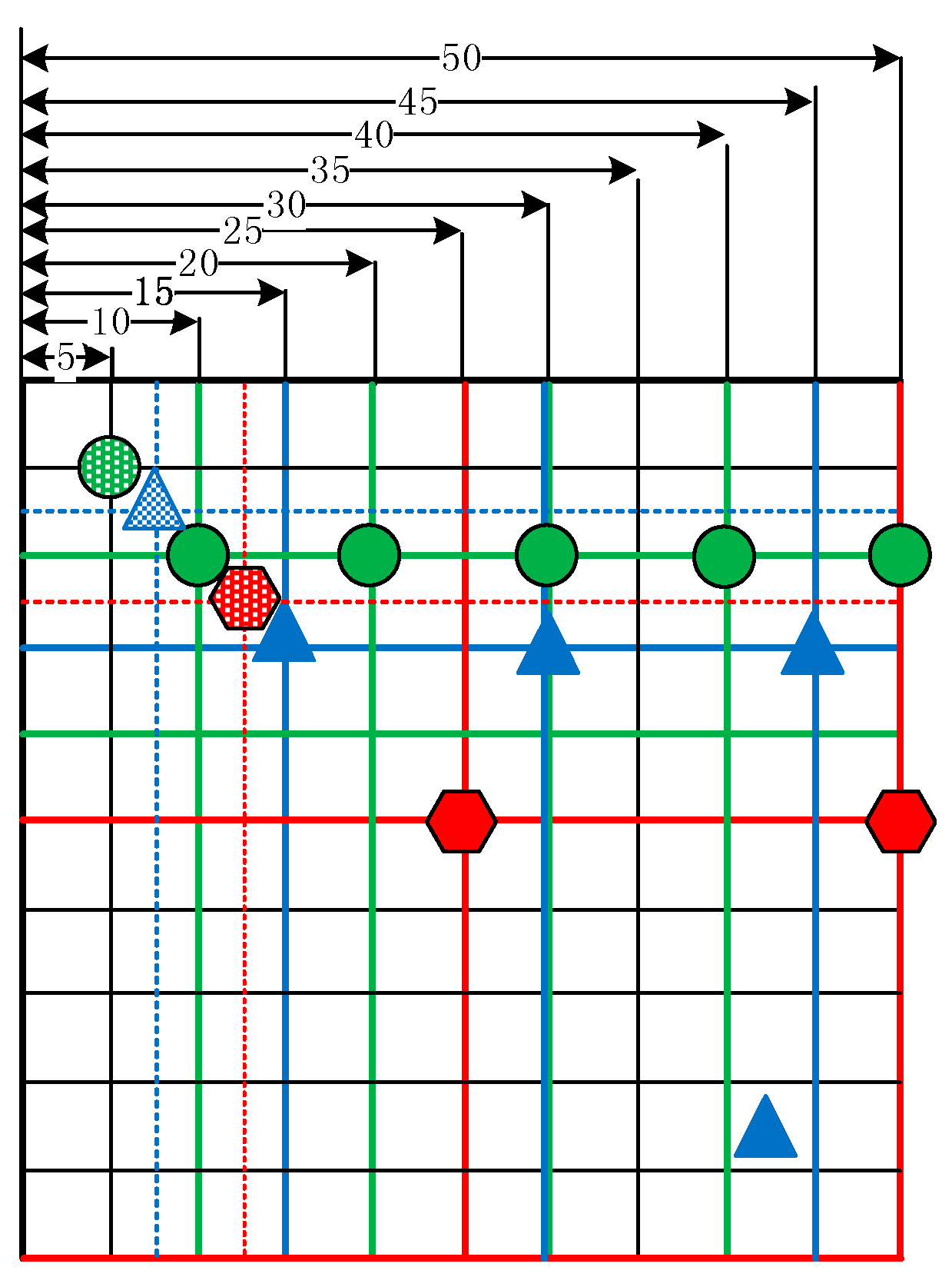
The coverage rate vibrates, which is shown in
Figure 8,
Figure 9 and
Figure 10. The points filled in red, blue and green in
Figure 11 are the grid points, which the FOV is divided into with the certain initial grid size of 25, 15 and 10. In addition, the corresponding sub-grid points are filled in with similar colors. As shown in
Figure 11, the sub-grid points need to be judged with initial grid size of 25, 15 and 10 not overlapping. Consequently, the status of each grid point is not the same, and then the coverage rate vibrates as shown in
Figure 8,
Figure 9 and
Figure 10.
4.3. Real Geographic Environment Data
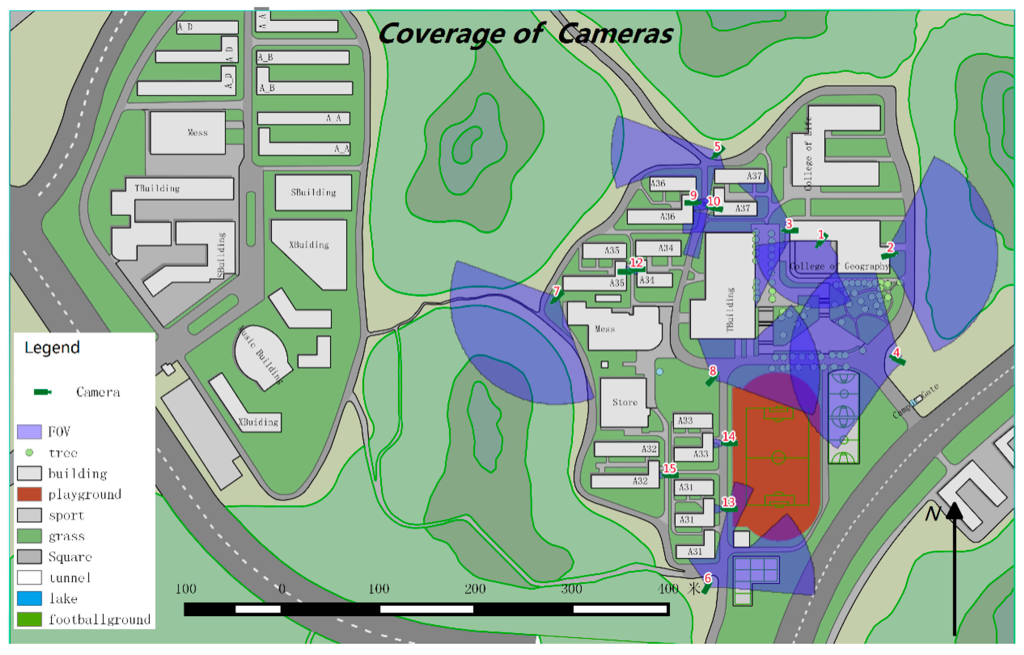
As illustrated in
Figure 12, there are 15 cameras deployed, including eight PTZ (Pan/Tilt/Zoom) ones and seven still ones. PTZ cameras can rotate and tilt at a certain angle and provide optical zoom; therefore, their coverage is a sector composed of the coverages from all possible camera positions. In the experiment, the steps for pan and tile are one degree. If the pan and tile range are (230,310) and (25, 65) respectively, then the coverage is estimated 3200 times. Consequently, the point numbers of PTZ cameras is the sum of point numbers from cameras with certain pan and tile. The still camera’s coverage is a quadrangle. All the camera parameters are listed in
Table 2. Their locations and coverages are illustrated in
Figure 12. The digits in red represent the ID of the camera, and the areas in transparent blue are the coverages estimated by our proposed method. In the experiment, the buildings are the major obstacles because the height of the cameras is much lower than building height. There are 85 features in the building layer.
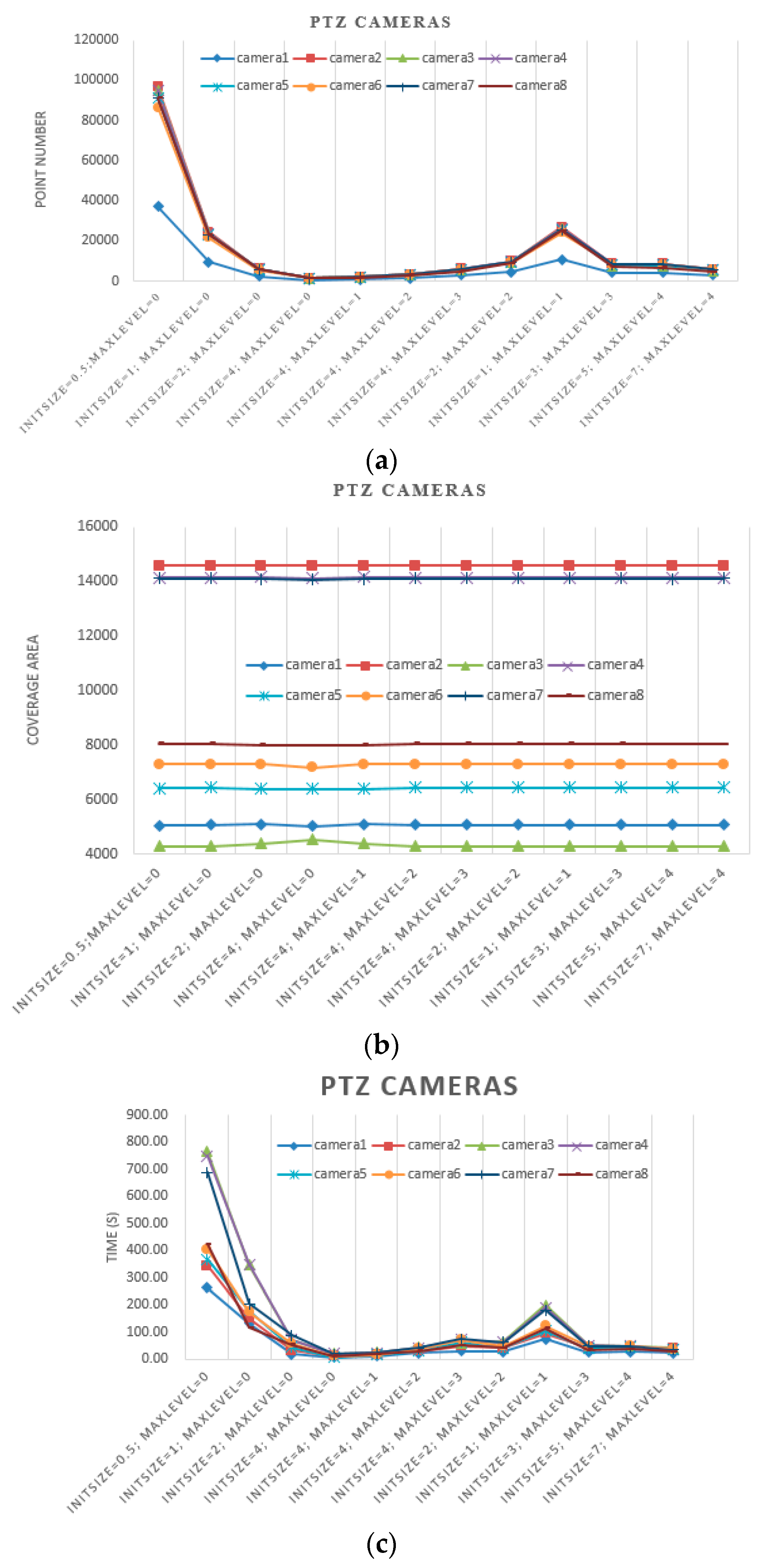
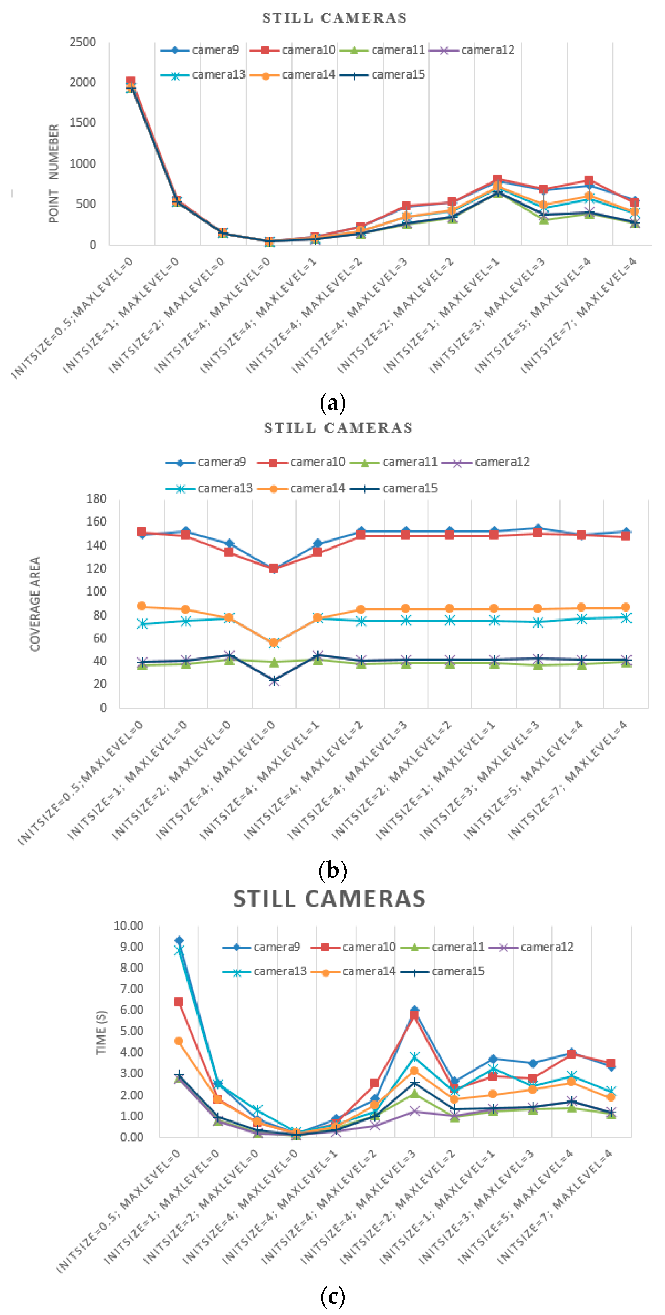
In this experiment, we first set the initial grid size to 4, 2, 1 and 0.5 m. Then, we estimated camera coverages without further subdivision. Second, we set the initial grid size to 4 m and set the max level to 0, 1, 2 and 3. Third, we set the size of the grid max level to 0.5 m. In other words, we set the initial size and max level as 4 m and three levels, 2 m and two levels, 1 m and one level, and 0.5 m without subdivision. Because of ignorance of the ground truth, we compared our estimated results with ones taking 0.5 m as the initial grid size and 0 level as the max level. Because of differences in the order of magnitude, the results of PTZ cameras and still cameras are illustrated in
Figure 13 and
Figure 14, respectively.
From the results illustrated in
Figure 13 and
Figure 14, the same conclusions can be made as with the experiment with simulated data, along with the following considerations:
- (a)
When the size of the grid in max level is the same, which is 0.5 m for example, the initial size and max level are set as 4 m and three levels, 2 m and two levels, 1 m and one level, the point numbers increase with the initial grid size, and they are significantly lower than results with 0.5 m as the initial grid size and 0 as the max level. However, the coverage areas are close to the ground truth.
- (b)
When the size of the grid in max level is similar, for example, the initial size and max level are set as 3 m and three levels, 5 m and four levels, 7 m and four levels, the point numbers and coverage area are close to each other.
- (c)
On one hand, the point number depends on the camera’s physical coverage, which is influenced by camera parameters and geographic environment. As the physical coverage increases, the point number increases. On the other hand, the point number is influenced by the initial grid size together with the max level proposed by our method.
- (d)
As shown in
Figure 13c and
Figure 14c, with the same initial grid size, the processing time of different cameras increases as the max level increases. With the same max level, the processing time increases with the initial grid size. When the size of the grid at the max level is the same, the processing times of different cameras are close to each other. Even though the point numbers of different cameras are close to each other, the processing times vary. Moreover, the processing times of different cameras vary because of their locations, poses and obstacles.
- (e)
The processing times of PTZ cameras is very time-consuming because the total coverage is combined with lots of coverages estimated with certain pan and tile.
5. Analysis and Discussion
The accuracy and efficiency of our proposed method are greatly influenced by camera parameters, obstacles, initial grid size and max level. The camera parameters can be employed to estimate the FOV in the theory, and obstacles must be considered when physical coverage is needed. However, it is hard to make a quantitative analysis of the influences before camera deployment. In general, cameras for city public security are usually deployed in entrances, exits and road intersections for monitoring moving targets. The geographic environment with obstacles such as buildings and trees is simpler than the simulated five-star. Consequently, in the paper, we emphasized the later factors: the initial grid size and the max level.
We use
and
to represent the row and column number of grid points from subdivision of the MBR with unified grid size
, where
is the initial grid size, and
is the current subdivision level:
Therefore, the number of grid points from subdivision of the MBR with unified grid size
, which is written as
, is computed by Equation (5) with
. The number of grid points from subdivision of the MBR with unified grid size
is written as
in Equation (6). In theory, the number grid points should be estimated in the proposed method with initial grid size
and max level
l, which is written as
, not less than
and not bigger than
That is,
:
Consequently, the time complexity of our algorithm is O(). To avoid judging the status of gird point repeatedly, our method needs to record the judged grid points. Consequently, the space complexity is also O(). In reality, when the camera is deployed in an environment with complex occlusions, the efficacy of the proposed method is close to . When the camera is deployed in a relatively flat area with few obstacles, the proposed method is more efficient.
On average, our method trades off efficacy and accuracy. Experiments with simulated and real data reveal the same conclusions. Overall, the oversize initial grid results in less accuracy, and the oversize max level is less efficient without obvious accuracy improvement. An undersize initial grid results in more computing time, and the undersize max level could cause less accuracy. Consequently, it is important to choose a proper combination of the initial grid size and max level. In application, there are three suggestions resulting from our experiments:
- (1)
If high efficacy is given priority over high accuracy, a larger initial grid size and smaller max level should be chosen.
- (2)
If high accuracy is given priority over high efficacy, a smaller initial grid size and larger max level is appropriate.
- (3)
When the focus is a balance between accuracy and efficacy, the parameters can be determined by the following steps: (a) roughly estimate the FOVs in theory and their MBRs; (b) estimate the smallest grid size and max level for the desired accuracy; and (c) estimate the initial grid size and max level for acceptable efficacy and accuracy using Equations (5) and (6).
In this paper, there are some limitations. This is unavoidable when sampling. In theory, if the grid size is small enough, a best grid approximation will be obtained, but it is impractical to divide the area infinitely. It is usually divided into grids according to practical requirements.
(1) If the initial grid size is not small enough, our method may ignore the conditions, which are illustrated in
Figure 15. When the grid coded as (1111) has a few holes, its geometry and area are overestimated. When the grid coded as (0000) has a few islands, its geometry and area are underestimated. To avoid or reduce the impacts of sampling without loss of computing efficiency, it is suitable to choose a relatively smaller initial grid size and then determine the max level according to the desired deepest grid size. The conditions shown in
Figure 15 are infrequent.
(2) The efficacy and accuracy of our method is affected by boundaries. As shown in
Figure 5 and
Figure 6, the boundary of physical coverage is not perpendicular to the vertical or horizontal direction. Therefore, the estimated coverage is serrated, and the grids crossing the boundary need to be divided by the max level to approach the physical coverage, which may cause more computing time.
(3) The monitored area in our method is flat ground, some errors may result when the area is rolling, and a few points may be occluded by the terrain. Our method can be improved for 3D terrain because its core for a visibility test is LOS when high precision DEM/DSM is accessible.
6. Conclusions
In this paper, a method is proposed to estimate camera coverage that balances accuracy and efficacy. In this method, the camera FOV in theory is divided by grids of different sizes with on-demand accuracy rather than by grids with one fixed size. Accuracy is approximately equivalent to the method employing the same deepest grid size, but efficacy is equivalent to the method employing the same initial grid size. It is suitable for a camera network, which contains hundreds of cameras and needs to obtain coverage frequently because of reconfiguration, coverage enhancement, optimal placement, etc. In this paper, we employed the LOS to estimate the visibility of the grid corner points. Even though the experiments cater to 2D areas with obstacles in vector format, it is easy to expand to 3D camera coverage when the high-precision grid DEM is available. In addition, different LODs of 3D buildings will be considered in our future works.


