An Efficient Query Algorithm for Trajectory Similarity Based on Fréchet Distance Threshold

Abstract

The processing and analysis of trajectories are the core of many location-based applications and services, while trajectory similarity is an essential concept regularly used. To address the time-consuming problem of similarity query, an efficient algorithm based on Fréchet distance called Ordered Coverage Judge (OCJ) is proposed, which could realize the filtering query with a given Fréchet distance threshold on large-scale trajectory datasets. The OCJ algorithm can obtain the result set quickly by a two-step operation containing morphological characteristic filtering and ordered coverage judgment. The algorithm is expedient to be implemented in parallel for further increases of speed. Demonstrated by experiments over real trajectory data in a multi-core hardware environment, the new algorithm shows favorable stability and scalability besides its higher efficiency in comparison with traditional serial algorithms and other Fréchet distance algorithms.

1. Introduction

With the rapid development of mobile internet, various types of sensors on mobile devices record diversified information of their carriers, personnel or equipment’s track of locations, which are the most common types of data of great value in many location-based applications. Accordingly, the processing and analysis of trajectory data has emerged as a critical area of development in the field of geographic information and data mining. In this case, the similarity measure and similarity query of the trajectory are the basis of many analytical processes. Since the absolute value of the trajectory distance has different practical significance with a different definition, it is often used as a filter or classifier. Furthermore, the trajectory data of the actual object inevitably has a noise disturbance. Therefore, in most cases, a query result set which is within the threshold of a given distance to the target can comply with the requirements of applications.

The similarity of trajectory is useful to many applications in the field of production and habits of public, policy-making of government, market research, and product promotion of commercial companies. For example, people with a similar work schedule and a frequent action trajectory in a region can be taken as the reference of group classification [1,2], which is an important factor to consider for administrations’ policy-making or infrastructure construction, while the business sector can use the data for accurate advertising and product designing. Moreover, in the field of cosmic astronomy, a large amount of orbital data can be obtained through the telescope, and using a simple distance threshold query, we can get a rough division of the countless galaxies and even the relative structure inside a single galaxy [3]. However, due to the complexity of the trajectory similarity calculation and the large-scale of the actual trajectory dataset, the efficiency of the existing algorithm is far from practicable.

Based on the summary of research status of the trajectory similarity computation, a fast query algorithm called the OCJ algorithm is proposed in this paper to address the problem of Fréchet distance threshold filtering ona large-scale trajectory dataset. Using a pre-filter operation based on the shape feature of trajectory and a sequential coverage judgement, the result set within the Fréchet distance threshold is obtained quickly. The algorithm can be optimized in parallel to achieve further increases in speed. Experiments show that OCJ algorithm has not only high query efficiency but also good running stability and scalability. Thus it is concluded that, compared with traditional serial algorithm and other Fréchet distance algorithms, the parallel OCJ algorithm has lower computational complexity.

2. Research Status

The original definition of the trajectory is the curve formed by the continuous change of a moving object’s position over time in the Euclidean space. However, the trajectory data obtained in the practical application is generally an ordered point of position, which is essentially a sampling result of the real continuous trajectory at a certain frequency over a certain period of time. In the geographic information system, it is often based on this point set to generate line data for description and visualization of a moving object’s trajectory. The algorithm proposed in this paper is based on the discrete trajectory data described above.

The similarity query of the trajectory contains two levels of the problem. One is the choice of the distance measurement of the trajectory, and the other is the algorithm to find the trajectory within the threshold. Trajectory data differs from simple line data in the strict order of interior nodes, so there are many schemes for the measurement of the trajectory distance, including the maximum distance, the minimum distance, the average distance, Hausdorff distance, Fréchet distance, Dynamic Time Warping (DTW), Longest Common Subsequence (LCSS) and Time Warp Edit Distance (TWED), etc. [4,5].

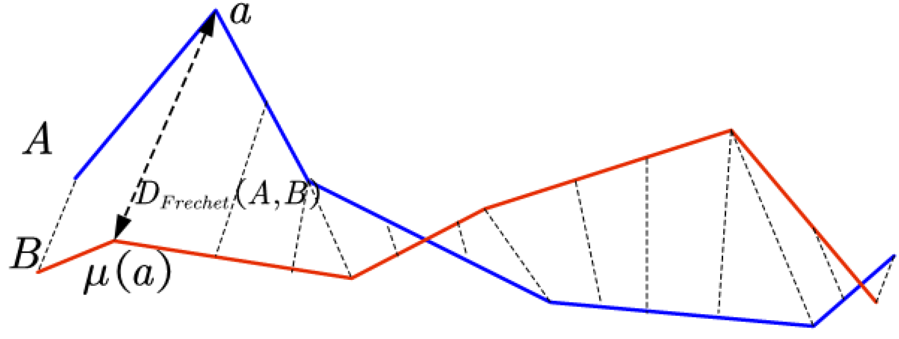
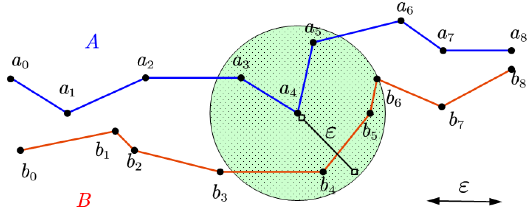
The definition of Fréchet distance is shown as Equation (1):

$$D_{Frechet}\left(A,B\right)=\underset{\mu }{min}\underset{a\in A}{max}d\left(a,\mu \left(a\right)\right)$$

(1)

where $\mu$: A→ B refers to a one-to-one continuous mapping from a point on trajectory A to a point on trajectory B.

Figure 1 shows an example of the Fréchet distance between two trajectories.

Previous studies have shown that the Fréchet distance contains the temporal relationship between the interior nodes [6]. Namely, the structure of the nodes inside the trajectory is taken into consideration in the computation process, which can more accurately describe the similarity between the trajectories. [4,5] For example, when there exists backward direction, ring or crisscross in a trajectory, the Fréchet distance value shows no distortion than other distance measurements. Hence, the Fréchet distance metric is more descriptive and more suitable as a measure of the similarity between trajectories.

2.1. Accurate Fréchet Distance Calculation

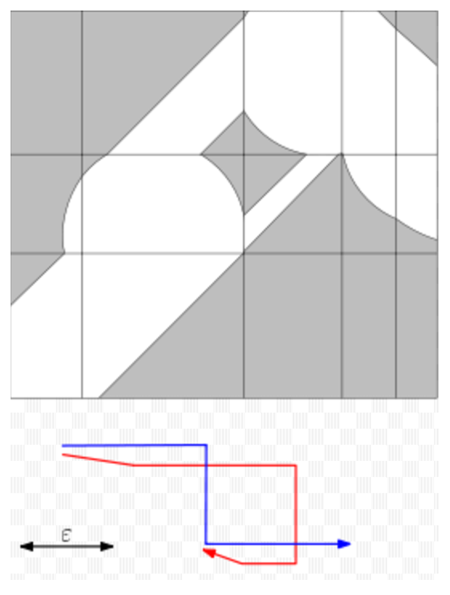
The exact Fréchet distance calculation is a NP hard problem [7]. There is no ideal algorithm with polynomial complexity to calculate a continuous curve’s Fréchet distance. Godau [7] proposed a graph describing the relationship between two trajectories in 1991 called Free-Space Diagram. On this basis, a method of calculating the trajectory of the polyline is proposed, namely, gradually reducing the value of $\epsilon$ until a path appears between (0, 0) and (p, q), where p and q are the lengths of the two trajectories (see Figure 2). The minimum value of the eligible $\epsilon$ is exactly the approximate Fréchet distance of the two trajectories and the computation complexity is O((p${}^2$q + pq${}^2$)logpq); Alt and Godau [8] improved the algorithm in 1995 by optimizing the strategy of searching for $\epsilon$ and successfully reduced the computation complexity to O(pqlogpq${}^2$).

2.2. Variants of Fréchet Distance

Eiter and Mannila [10] proposed a variant of the Fréchet distance called discrete Fréchet distance in 1994. They first approximate the trajectory into a set of ordered discrete points, and then compute the maximum distance of the discrete point pairs. It is proved that the discrete Fréchet distance, whose computation complexity is only O(pq), is the upper bound of the continuous Fréchet distance [10]. However, they had not provided an implementation of the algorithm. This simplified model is more suitable for the actual trajectory data, and brings little measurement accuracy. Consequently, the latter research of the Fréchet algorithm is mostly based on the discrete Fréchet distance model, in which the Free-Space Diagram degenerates to the distance matrix between the track points. In 2013, Agarwal et al. [11] used the finite state machine method to find the path of the distance matrix, and deduced that the upper bound of the Fréchet distance can be attained in the complexity of O((pqloglogq)/log${}^2$(q)). Aronov et al. [12] suggested to first simplify the trajectory data by reducing the number of interior nodes and then calculate its Fréchet distance with a smaller n in computation, while Drierel et al. [13] introduced a new approximation to simplify the trajectory using a c-packed curve. A simple and practical (1 + $\epsilon$) approximation linear algorithm is proposed to calculate the approximate Fréchet distance of the trajectories [13]. Furthermore, Har-Peled et al. [14] proposed an approximation algorithm for a variant of Fréchet distance called homotopic Fréchet distance with O(logn) complexity, but the accuracy needs to be improved.

2.3. Fréchet Distance Threshold Query

In order to solve the problem of high complexity of Fréchet distance calculation, a distance matrix of two trajectories of the Convolutional Neural Network (CNN) is proposed by Sook Yoon et al. [15], which can make full use of CNN’s parallel computing ability. The complexity of judging whether the Fréchet distance to the reference trajectory is within a given threshold was reduced to O(max(p, q) − 1) [15]. Buchin et al. [16] divided the distance matrix of the two trajectories and constructs a dendritic lookup table to speed up the efficiency of traversing Free Space. The threshold query complexity was reduced to O(pq(loglogq)${}^2$/logq). For the retractable trajectory, Gheibi et al. [17] proposed a minimum recursive algorithm for weighted reentrant path based on the transformed Free-space diagram, with the complexity of O(pqlogq).

Bringmann and Karl [18] summarized the computational complexity of the Fréchet distance and its variants during the last two decades, and carried out analysis and derivation of the computation complexity theoretically under the Strong Exponential Time Hypothesis (SETH). It is pointed out that there is no strong quadratic function complexity solution within the error range of 1.001 [18].

In summary, it can be observed that the study of Fréchet distance mainly focuses on the simplification of the original definition and the design of the data structure for acceleration, but most research stopped after the theoretical design and derivation [19].

3. Problem Statement

Practical applications often need to screen out the eligible trajectories from a large-scale trajectory dataset which are within the Fréchet distance threshold to one or even more trajectories. To portray the problem more clearly, a basic description of the research and the definitions of the terms used in the following chapters are given below.

Target trajectory: the reference trajectory used to calculate distance;

Candidate trajectory: the trajectory to be judged if it is within the distance threshold with the target trajectory;

Totality problem: Finding the trajectories of the Fréchet distance from the target trajectory within the given threshold $\epsilon$ in the candidate trajectory dataset;

Subproblem: Judging whether the Fréchet distance of the two trajectories is within a given threshold $\epsilon$;

Distance: Unspecified distance refers to the ordinary distance, namely, the Euclidean distance in Cartesian space;

Nodes: An ordered discrete track point set that forms a trajectory, consisting of 2D or 3D coordinates and the time sequence relations of the points;

Trajectory length: The number of nodes/track points in the trajectory;

Segment (Seg): A directed line segment formed by two adjacent nodes, and a trajectory is the connection of a number of segments;

Link: A connection can be established between two nodes in the two trajectories if and only if the connection relation does not violate the timing sequence relationship of the whole trajectory. In other words, if a node is at the rear, its connection node is also located in the posterior position of the time sequence, which is the manifestation of Fréchet distance’s internal property of time ordering. It is similar to the concept of coupling in [9]. In particular, it is considered that the connection node of the head/tail of one trajectory is exactly the other trajectory’s head/tail;

Valid link: If the distance between two linked nodes is less than the given threshold value, the link is regarded valid;

Coverage: For node “a” in trajectory A, there is one or more nodes denoted as “b${}_i$, b${}_i+1$, …, b${}_j$” on track B can establish valid links with “a” (where 0 ≤ i ≤ j ≤ L${}_B$ , L${}_B$ is the track length of B). Namely the coverage of “a” is b${}_i$, b${}_i+1$, …, b${}_j$.

Example: As shown in Figure 3, A and B are two trajectories, $\epsilon$ is the given threshold, and the coverage of node a${}_4$ is b${}_4$, b${}_5$, b${}_6$.

4. OCJ Algorithm

As demonstrated in the problem description, the solution of the subproblem is the key component of the algorithm. According to the definition of Fréchet distance, it is necessary to find a full connection so that all nodes in A and B have corresponding link nodes. In theory, there are myriad ways to link the two trajectories and, in each way, there is a maximum length of the link, which is denoted as Dlink. Additionally, the Fréchet distance is the minimum value of Dlink. The problem can be transformed to one of determining whether the valid links of the target trajectory can cover the candidate trajectory following the restriction of time order.

OCJ is the abbreviation of Ordered Coverage Judge. The core idea of the algorithm is to calculate in an orderly fashion the coverage on candidate trajectory B of each node in target trajectory A by a given threshold, until all the nodes in A are traversed. If the coverage is ordered continuously and its union can cover all nodes in trajectory B, it could be judged that candidate B satisfies the query criteria.

4.1. Pre-Filter Based on Morphological Characteristics

By analyzing the Fréchet distance, some useful query filtering approaches can be obtained. Before running the OCJ algorithm, some pre-filtering operations can be performed based on the morphological characteristics of both the target trajectory and the candidate trajectory to reduce the number of trajectories to be queried. Specifically, there are three methods as follows:

4.1.1. Head/Tail Node Filtering

According to problem description, the link node of a trajectory’s head/tail node is exactly the candidate trajectory’s head/tail point, so the distance between the head/tail points must be less than the threshold to meet the query criteria. Therefore, the head/tail point filtering can be the first round of the pre-filter operation. To implement it, a spatial index like R-tree based on the first and last point is needed to accelerate the space query process. The steps are as follows:

• Build the R-tree index for head and tail node of the candidate trajectory respectively;
• Generate two square query boxes with 2$\epsilon$ as the edge length and target trajectory’s head/tail node as the center;
• Use the query boxes to query on the R-trees, respectively, and take the result set as the new candidate trajectory set.

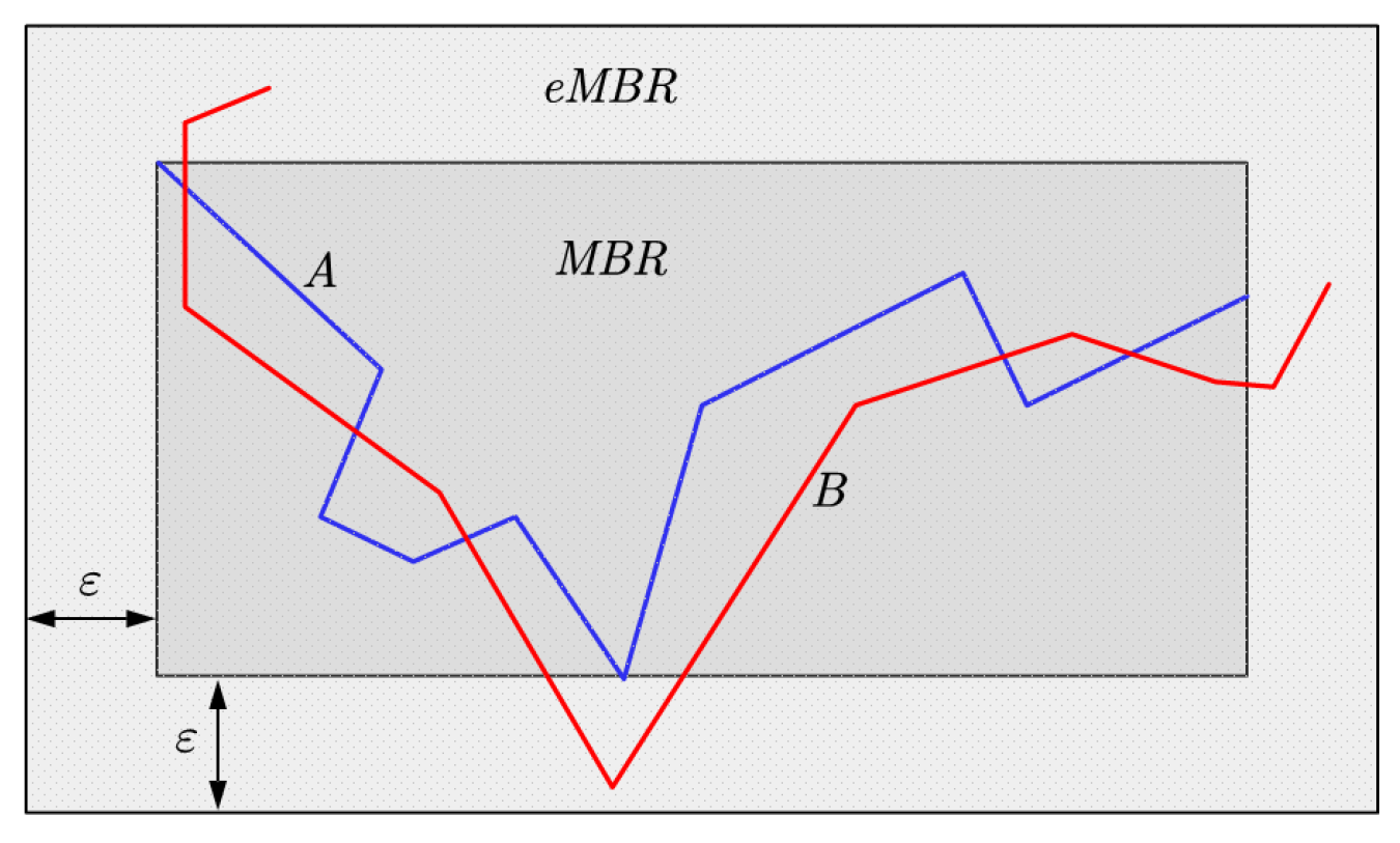
4.1.2. Minimum Boundary Rectangular (MBR) Filtering

As shown in Figure 4, the MBR of the target trajectory is extended by $\epsilon$, and the candidate trajectory that satisfies the query criteria must be located in it. Therefore, the MBR filtering could make the scale of candidate set further smaller.The filtering steps are as follows:

• Compute the MBR of the target trajectory;
• Extend the MBR of the target trajectory by $\epsilon$ to form the extended MBR (eMBR);
• Judge whether the candidate trajectory is located inside the eMBR using space containing function, and retain the candidate trajectories that satisfy the criteria as the new candidate set.

4.1.3. Buffer Filtering

This method is similar to MBR filtering in principle and procedure, except that the basis of filtering is replaced by the target trajectory’s buffer area which is more accurate in describing spatial location than MBR.

Buffer filtering also shares much similarity in implementation with MBR filtering, but it can figure out the trajectories containing more sharp inflection points and detour edges. So, its filtering effect is better than the MBR filter, but the calculation quantity grows at the mean time. In practical applications, they can be replaced by each other, or can also be cascaded with the others as a tradeoff between efficiency and effectiveness.

4.2. Synchronistical Ordered Coverage Judgement

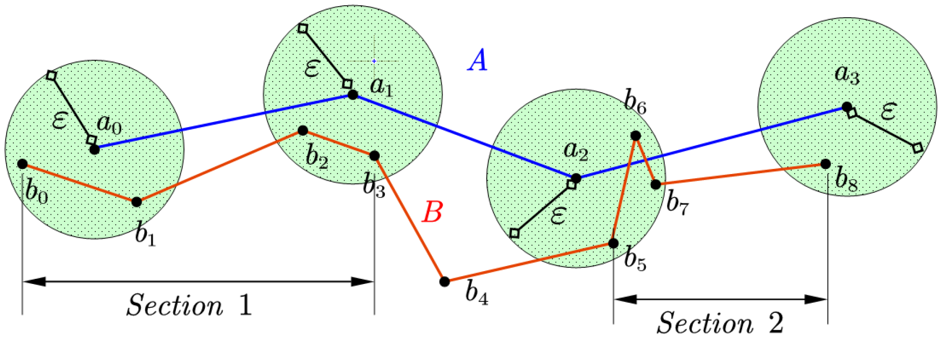
The core ofthe OCJ algorithm is the search of valid links and the sequential judgement of nodes’ coverage, and the operations can be synchronized in implementation. The following example illustrates the process.

The search for the valid links of the nodes in trajectory A is performed as

Table 1. Result of Valid link search.

Nodes in Trajectory A	Corresponding Linked Nodes in Trajectory B
a${}_0$	b${}_0$, b${}_1$
a${}_1$	b${}_2$, b${}_3$
a${}_2$	b${}_5$, b${}_6$, b${}_7$
a${}_3$	b${}_8$

:

As shown in Figure 5, a section consists of several adjacent segments and the search results consists of two sections: {b0, b1, b2, b3} and {b5, b6, b7, b8}. The b4 node is omitted so that the result cannot cover the entire candidate trajectory B. Therefore, trajectory B does not meet the query criteria. In the implementation, the search process and judgement are carried out synchronously. When the program traverses to node a2 in the above example, it is found that the coverage and the result of the preceding nodes are not connective. The search can be terminated immediately and return a negative result, without having to calculate the coverage of the remaining nodes. Pseudo-code of OCJ algorithm is as Algorithm 1.

In addition, when carrying out a real data experiment, it is found that a single node may correspond to a multi-segment coverage which is discontinuous. Assuming the coverage consists of seg1 and seg2, the valid link of the next node may start from the interval between seg1 and seg2 on the condition that the link satisfies the restriction of continuation with seg1, but not with seg2, which probably occurs when the trajectory is distorted. The algorithm could simply save the first segment of each node’s valid link for next node’s judgement, but in order to improve the search efficiency by stretching the coverage range faster, the OCJ algorithm adds a stack structure. With the valid coverages of the current node all pushed in, the stack will pop up former valid coverage for the discontinuous node to do the OCJ search again. Negative results will not be returned until the stack is empty.

4.3. Complexity Analysis

In the most undesirable situation, the OCJ algorithm needs to calculate the valid links for all nodes of the target trajectory, and each node’s valid link search progress needs to judge the distance to all the nodes from the candidate trajectory, while the continuity judgement’s complexity is merely O(1). So, assuming p and q to be the lengths of the two trajectories, the total computation complexity of the OCJ algorithm is O(pq), consistent with the complexity of the discrete Fréchet distance proposed by Eiter and Mannila [10]. However, in the process of carrying out the algorithm, if the candidate trajectory does not meet the query criteria, the search and judgement can be terminated as long as the node coverage’s continuity is interrupted. Therefore, in most cases the calculation cost is less than O(pq).

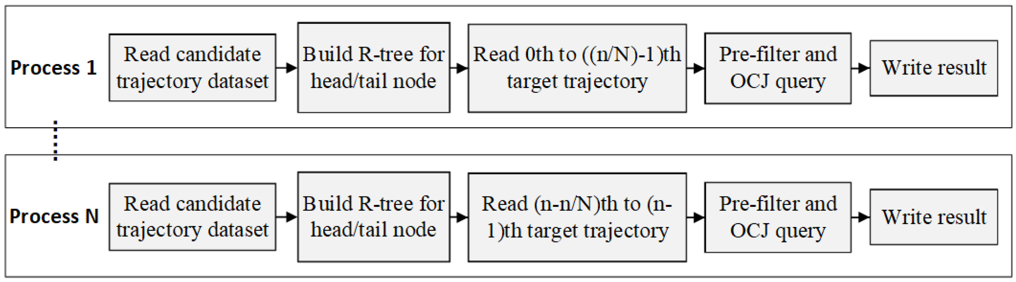
4.4. Parallel Optimization

An important factor in measuring an algorithm is whether it can be easily implemented in parallel to take full advantage of modern multi-core hardware environments, so it is necessary to optimize OCJ algorithm by parallel strategy design.

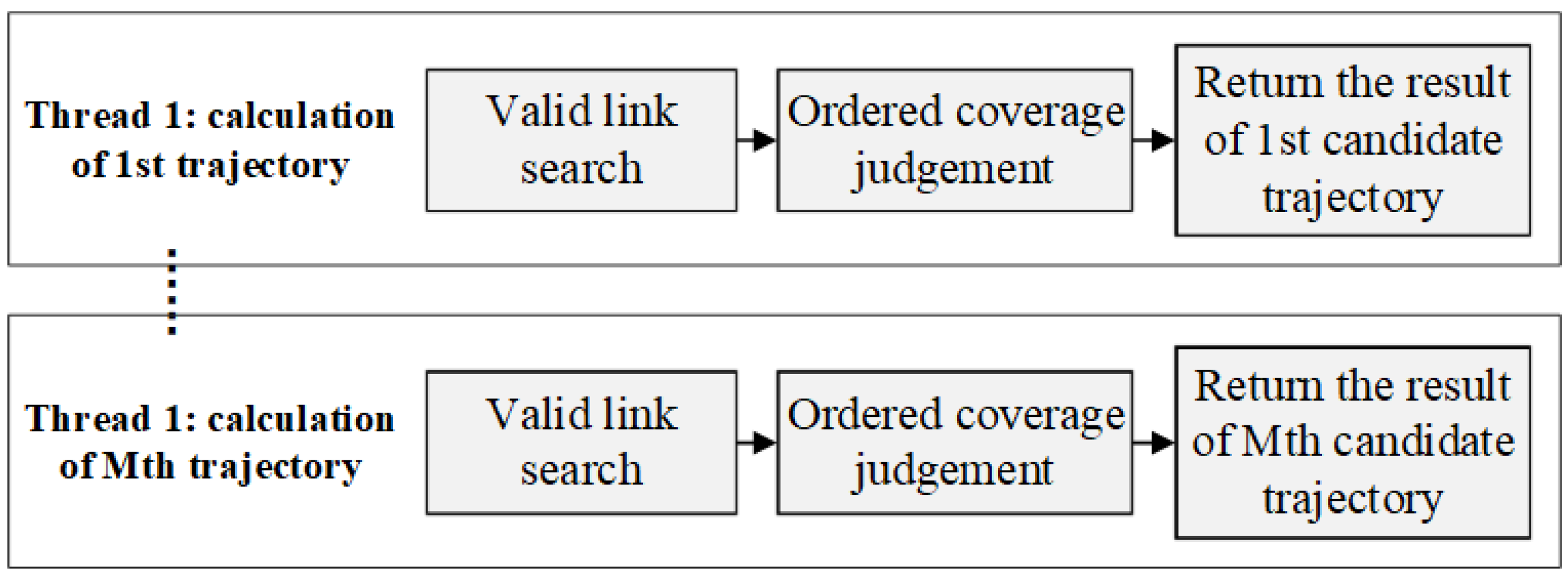
Considering that the target dataset and the candidate dataset often contain a large number of trajectories, it is sensible to combine parallel threshold query of multiple target trajectories and parallel ordered coverage search of a single target trajectory based on multiple processes and multiple thread. The parallel tragedy is illustrated by Figure 6 and Figure 7.

There is no data dependency between the query tasks based on different target trajectory, and the single judgement operation in the same query uses the same pair of trajectories, so OCJ algorithm is suitable to execute in a Massive Parallel Processing (MPP) environment. To demonstrate the parallel strategy, the algorithm is implemented based on both MPI + OMP parallel framework and the Spark distributed computing platform respectively. In the following section, the two approaches of implementation are compared and analyzed by real trajectory experiments.

5. Experiment and Analysis

The experimental dataset is extracted from real track data of taxi trips, which contains more than 20,000 trajectories. Each trajectory contains 10 to 1000 track points. It is a sample of T-Drive trajectory dataset that contains a one-week trajectories dataset of 20,200 taxis. The total number of points in this dataset is about five million. The download link of the dataset is shown in the Appendix.

The experiment’s environment is ubuntu16.04 LTS operating system, Intel^® Core ™ i7-4710MQ CPU (4 cores) @ 2.50GHz, 16GB RAM, 500GB HDD. The software environment is shown in

Table 2. MPI and Spark environment.

Item	Version
MPI Framework	MPICH2 3.2
MPI language	C++ 11
MPI compiler	GCC/G++ 5.4
Spark Platform	2.1.0
Spark language	Scala 2.12
File System	HDFS 2.7.3

.

5.1. Algorithm Stability

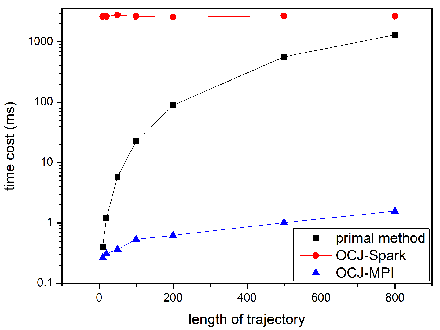
Firstly, the single-pair trajectory experiment of OCJ algorithm is carried out to evaluate the stability. By controlling the length of trajectory pair and comparing the time cost of the two implementations with the traditional algorithm, the experiment resulted in distinct patterns of performance as the line chart shown in Figure 8:

As illustrated in Figure 8, with the increase of the trajectory length, the efficiency of the OCJ algorithm in the Spark platform remains basically the same. This is because the distributed computing platform needs time to carry on the complex data structure, the parallel task division and the parallel resource scheduling before running the actual algorithm, even if the task quantity is very small. The preparation time almost stays the same and the calculation cost of the distance judgement of the single-pair trajectory is almost negligible compared with it, so the total task execution time is hardly affected by the trajectory length. Meanwhile, the OCJ algorithm implemented by the MPI parallel framework shows different performance in that with the increase of the trajectory length, the calculation time grows in a stable linear manner. Obviously, the traditional algorithm’s time cost grows much more steeply. It is evident that for the single-pair trajectory Fréchet distance threshold judgement task, the OCJ algorithm implemented in the MPI framework has a significant advantage in terms of computational efficiency.

5.2. Parallel Efficiency

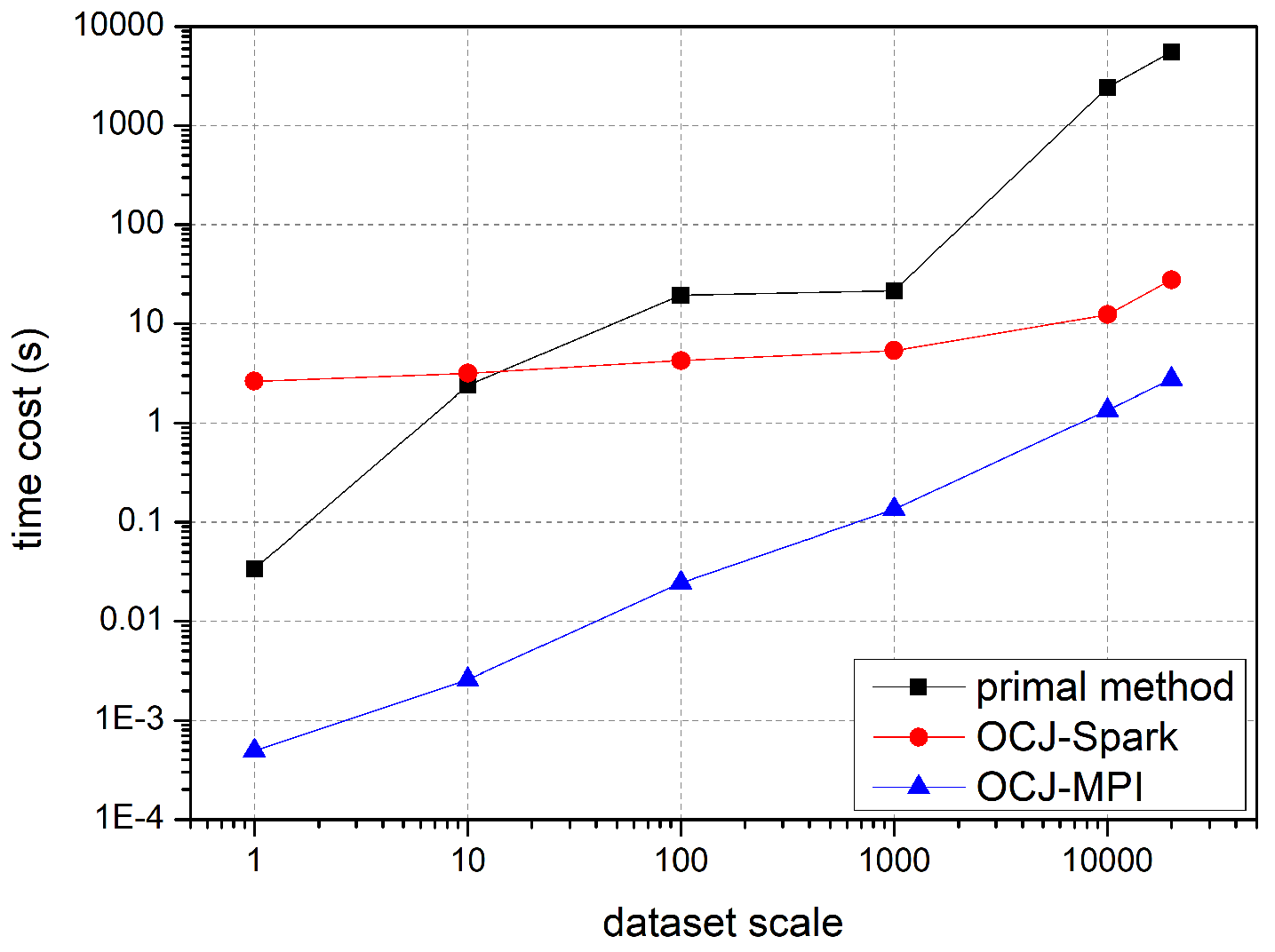
The scalability of the algorithm is an important performance index in the modern multi-machine and multi-core parallel computing environment, and the query based on distance threshold on two large-scale trajectory datasets is a common application scenario frequently used. Therefore, it is necessary to set the data set in a different scale to test the parallel efficiency of OCJ algorithm. The experiment’s results are indicated below.

As Figure 9 shows, the traditional algorithm costs hours when dealing with a large-scale query, far from the requirement of practical applications. Spark platform organizes trajectory data through a well-designed structure called Resilient Distributed Datasets (RDD), which is more suitable for running large-scale tasks on high-performance computing clusters. However, algorithms implemented in Spark consumes much more memory and cost longer initial times. As for the MPI implemented OCJ algorithm, it shows stable performance and good scalability with moderate memory consumption. Moreover, with the increase in the amount of trajectories, the OCJ-MPI algorithm achieves a nearly ideal speedup ratio.

It can be seen that both implementations of OCJ algorithm have a performance improvement of two to three orders of magnitude over the original violent algorithm when the dataset contains more than 10,000 trajectories, which illustrates that the parallel acceleration is quite effective. To further measure the acceleration effect of the algorithm, a parameter called “throughput index” is defined by Formula (2):

$$Throughput=\frac{L^2}{C_p/C_1}$$

(2)

where L represents the number of trajectories contained in the dataset, and the L value of target datasets and candidate datasets grows synchronously in this experiment, so L${}^2$ can represent the total computational magnitude; C_p represents the time cost when parallel process number is p; and C${}_1$ represents the time cost of a serial execution. The throughput index can roughly measure the parallel effect of the parallel algorithm quantitatively as the computation magnitude increases.

It can be seen from

Table 3. Throughput rate.

Scale of Trajectory Dataset	1	10	100	1000	10,000	20,000
Throughput index of Spark	1	83.021	6185.981	489,631.98	21,202,071	21,917,923
Throughput index of MPI	1	22.934	244.444	4400	43,934.91	86,305.85

that although the Spark platform is much more computationally expensive than MPI, its throughput strategy has obvious advantages, that is, its parallel acceleration potential is greater, and it can be inferred that in the larger data set experiment, Spark’s performance is likely to exceed the MPI implementation. Of course, it requires a computing cluster to provide enough memory for Spark.

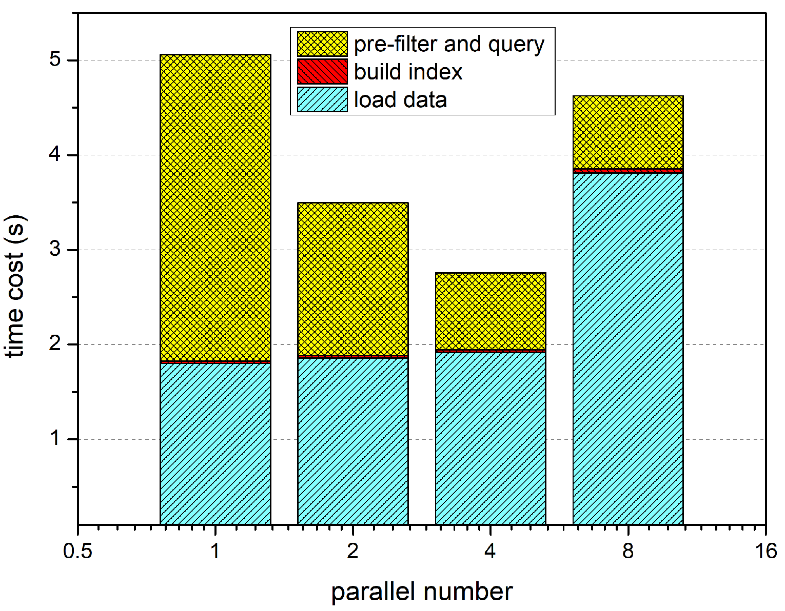
5.3. Time-Consuming Proportion

This subsection gives a specialized analysis for the MPI implementation of the OCJ algorithm. The OCJ algorithm mainly includes three stages: data IO, head/tail node index construction, and filter query. The query is the main calculation process and consists of pre-filtering, valid link search and ordered coverage judgement. In order to further optimize the algorithm, it is necessary to analyze the time-consuming proportion of each part of the algorithm. The test task is to perform the Fréchet distance threshold query on the target dataset and the candidate dataset both containing 20,000. The control variable is the number of running processes, and the recording variable is the proportion of each part in the total time cost. The results are as Figure 10:

It can be seen that when the number of processes is less than the number of CPU cores, with the increase of the number of processes, the R-tree construction time almost stays the same and query time is linearly decreasing. The acceleration effect of query is obvious because the operation mainly includes the valid link search and continuous coverage judgement process which are both computationally intensive. In addition, there is no data dependency between the query operations over different trajectories, so it is very suitable for multi-process parallelism.

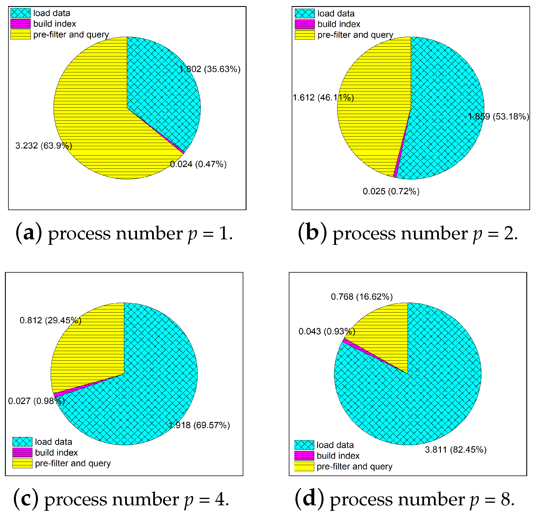
When analyzing the data loading phase, each process needs to load all the candidate trajectory dataset for a complete search. As declared in the beginning of Section 4, the program was run on a four-core desktop, which means that four different processes can be executed homochromously. So, the load time almost remains the same when the parallel number is less than four (the core number of CPU). However, when the parallel number is eight, double the core number of CPU, the reading process have to queue for their data, which results in the rise of loading time. Although by means of parallel read, cache acceleration and other hardware optimization measures, the total data IO time still occupies the majority of total time cost, and the greater the number of processes, the higher the proportion of data IO occupies. This phenomenon is demonstrated more clearly in the pie charts in Figure 11.

The result inspires that the next step of optimization of the algorithm is to design a more efficient parallel trajectory dataset reading method or strategy.

6. Conclusions and Discussion

Fréchet distance takes into account the temporal relation of the internal nodes in the trajectory, and the similarity of the trajectories can be better described than other distance measures. Therefore, the filtering query problem based on Fréchet distance has a wide range of practical applications. In this paper, the proposed OCJ algorithm can quickly solve the Fréchet distance threshold query problem by pre-filter pruning, valid link searching and ordered coverage judging based on trajectory characteristics, and can be parallelized expediently using MPI framework to achieve efficient acceleration. The experiment based on large-scale trajectory dataset shows that the OCJ algorithm and its parallel implementation have better computational efficiency and good parallel expandability, which is of considerable value in practical applications.

However, if the search threshold is lower than the longest segment of either of the two trajectories, some trajectories meeting the query criteria will be discarded. It is the loss of precision caused by simplifying a continuous curve to a discrete polygonal line. Although in practical datasets, the trajectories usually have enough sampling density to avoid this kind of discarding, we have to design a strategy for extreme query cases. Linear interpolation of the long segment may solve the problem.

Furthermore, the OCJ algorithm can only judge whether the Fréchet distance of the two is within a given threshold and has some limitations for further application. In the future work, it will be meaningful to combine an efficient and parallel capable threshold search algorithm with OCJ to obtain the exact Fréchet distance between the trajectories, which will produce a better application prospect.