A Novel Approach to Semantic Similarity Measurement Based on a Weighted Concept Lattice: Exemplifying Geo-Information

Abstract

The measurement of semantic similarity has been widely recognized as having a fundamental and key role in information science and information systems. Although various models have been proposed to measure semantic similarity, these models are not able effectively to quantify the weights of relevant factors that impact on the judgement of semantic similarity, such as the attributes of concepts, application context, and concept hierarchy. In this paper, we propose a novel approach that comprehensively considers the effects of various factors on semantic similarity judgment, which we name semantic similarity measurement based on a weighted concept lattice (SSMWCL). A feature model and network model are integrated together in SSMWCL. Based on the feature model, the combined weight of each attribute of the concepts is calculated by merging its information entropy and inclusion-degree importance in a specific application context. By establishing the weighted concept lattice, the relative hierarchical depths of concepts for comparison are computed according to the principle of the network model. The integration of feature model and network model enables SSMWCL to take account of differences in concepts more comprehensively in semantic similarity measurement. Additionally, a workflow of SSMWCL is designed to demonstrate these procedures and a case study of geo-information is conducted to assess the approach.

1. Introduction

In information science and systems, semantic similarity plays a major role in various fields such as information retrieval, data integration, data mining etc. [1,2,3]. Since its emergence in these fields, various theories on semantic similarity have been proposed [4]. At the same time, a large number of approaches based on these theories have been developed and utilized to measure semantic similarity [5,6,7,8]. The objects of semantic similarity measurement are usually called different terms, such as classes or concepts, across various articles. In this paper, the term ‘concept’ is used to represent the measurement object. The classical models of semantic similarity measurement, named feature models [9], are based on the representation of object-attribute knowledge, in which concepts are represented as a set of features and sometimes the relationships between them. Following this, semantic similarity can be translated into a comparison of the commonalities and differences of sets of features that represent different concepts. Some other semantic similarity measurement approaches are based on network models, which encode knowledge in a form of a semantic network [10]. Concepts in the semantic network are represented as vertices, which are connected with links. Thus, the ‘distances’ between vertices, which can be defined with various meanings, such as shortest path, weighted path length and so on, can be regarded as measurements of semantic similarity between concepts. Apart from these two main models mentioned above, some other models and approaches to measuring semantic similarity have been proposed [4,11]. Some new approaches aim to overcome the shortcomings of existing solutions by integrating different models [8,12].

Although many different models and approaches have been proposed to deal with this issue, there is no general model or approach, which is broadly applicable for all fields. This is partly because the methods used to judge semantic similarity are dependent on different factors, such as the application context, purpose etc. [13]. Most of the existing approaches are incapable of dealing with the issue of the dependence of semantic similarity judgment on different application contexts. Although some modern approaches take into account the influence of distinguishing contexts, they still cannot effectively assign weights to various factors, such as the semantic granularity of a concept and application context, which have different influences on semantic similarity judgment. With reference to various existing approaches, we propose a novel approach to semantic similarity measurement based on a weighted concept lattice (SSMWCL) in this paper, which combines both a feature model and network model. SSMWCL has the power to quantify the effects of different contexts on semantic similarity. Based on the knowledge representation of the feature model [9], SSMWCL first calculates the combined weight of each attribute of the concepts by merging its information entropy and the importance of its inclusion-degree in a specific application context. After this, our approach generates the weighted formal concepts using formal concept analysis and builds a network hierarchical structure, which is named the weighted concept lattice. In this lattice, the weighted concepts are represented as vertices linked with edges. Following this, the absolute semantic similarity between concepts is measured by comparing the commonalities and differences of their weighted attributes, in which the relative hierarchical depth of the concepts in the lattice is taken into account based on the principle of the network model. Finally, the semantic similarity is measured using the proportion of absolute semantic similarity in the semantic intent of the concept. Finally, the semantic similarity is normalized by introducing an exponential function. In our work, there are three main innovative points. The first involves transforming the impact of the specific application context on semantic similarity judgement into weights of attributes of concepts; the second includes integrating the feature model and network model in SSMWCL; while the third introduces the size of the concept intent’s weight as an influencing factor on semantic similarity judgement.

The remainder of this article is organized as follows: Section 2 provides a brief survey of work related to semantic similarity measurement, formal concept analysis and the weighted concept lattice applied in information science and systems. At the same time, we present a workflow of SSMWCL. In Section 3, we introduce relevant algorithms to construct a weighted concept lattice based on the knowledge representation of the feature model. For this construction, some mathematical tools are applied, including the rough set, information entropy, and formal concept analysis. In Section 4, a novel approach for semantic similarity measurement based on a weighted concept lattice (SSMWCL) is proposed, and an implementation workflow of SSMWCL is presented at the end of the section. Section 5 demonstrates a case of measuring semantic similarities of geo-concepts in accordance with the workflow of SSMWCL, and the results are discussed briefly. Section 6 summarizes our approach, qualitatively compares it to other similar methods, and presents an outlook for the future.

2. Background

The importance of semantic similarity in theory and practice has been acknowledged for decades in information science and systems, with increasing numbers of relevant studies having been conducted. Being first proposed and used in psychology [14], the geometric model regarded semantic distance (similarity) in the analogy of spatial distance. Semantic distance (similarity) in the geometric model is computed to be a function of spatial distance. On the basis of this model, Gärdenfors, Raubal and Schwering used conceptual spaces, which developed the geometric model to measure semantic distance [15,16]. Tversky et al. introduced and used a set-theoretical similarity measurement, nowadays known as the feature model. Based on the feature model, Rodriguez and Egenhofer proposed the matching-distance similarity measure (MDSM), which distinguished three different types of features of spatial entity classes to determine the semantic similarity of these classes [8]. Furthermore, Janowicz et al. developed SIM-DL and SIM-DLA theories, which tried to introduce description logics into the feature model [17,18]. Based on the network model that connects concepts to establish a semantic network, Ballatore et al. computed the semantic similarity of geographic concepts in the OpenStreetMap (OSM) semantic network [7]. Janowicz et al. proposed a generic framework for semantic similarity measurements in geographic information retrieval, which allows designers to compare and select different measurement approaches for the specific application [19]. Kim et al. matched place descriptions with overall similarity (including string, linguistic and spatial similarities), which can be regarded as combined semantic similarity [20]. More recently, some other theories have been introduced to measure semantic similarity. Francis-Landau et al. tried to capture semantic similarity for entity linking with a convolutional neural network, which is known as the machine learning approach [21]. Mihalcea et al. assessed the semantic similarity of the cross level with deep learning [22].

In this work, we focus on the semantic similarity measurement between a pair of concepts. In this specific field, four main sets of approaches are used to achieve this goal [23]. The most popular method is the structural approach which uses the network model and relies on graph traversal. The shortest path [24], random-walk [25] and other interconnections [26] between nodes are the main variables used to define the semantic similarity function. Based on the feature model, the feature-based approach [8,27] compares the commonalities and differences between a pair of concepts in order to obtain the semantic similarity. The information theoretical approach relies on Shannon’s information theory [28]. With this approach, the semantic similarity of concepts is measured by comparing their information context (IC) [29,30]. The hybrid approach takes advantage of various aforementioned paradigms. Singh et al. mixed the information theoretical and structural strategies [31]. Rodríguez and Egenhofer proposed mixing the structural approach and the feature-based approach [2]. However, the aforementioned approaches have several limitations. All these approaches require a taxonomy or ontology structure describing the elements to compare [23]. The structural approaches require knowledge to be modeled in a specific manner in the graph and are not designed to take non-binary relationships into account. That means different types of relationships among concepts cannot be distinguished and weighted. Feature-based approaches usually cannot assign different weights to different attributes according to the various application backgrounds. In our work, the proposed SSMWCL does not require an existing taxonomy or ontology structure. However, this does not mean that SSMWCL cannot work based on a taxonomy or an ontology structure. In fact, existing ontology will make it easier to implement the SSMWCL by conveniently extracting essential properties and the classification hierarchy of concepts. On the other hand, the SSMWCL approach enables the assignment of different weights to different essential properties of concepts based on the various application backgrounds. In order to distinguish the influence weight of essential properties of concepts for measuring semantic similarity, we first analyze and calculate the combined weights of properties of concepts by mixing feature-based and information-theoretical approaches. Following this, the depth of concept in the network structure integrated with the weights of features can be used to define the semantic similarity between a pair of concepts.

Formal concept analysis (FCA), proposed by Wille [32], has become an important branch of applied mathematics. Its application has expanded into various fields, such as linguistics, information science, software engineering, computer science etc. Integrating heterogeneous data or information from many sources is an important characteristic of FCA. Stumme and Adche developed the FCA-MERGE method, which entails building a concept lattice and semi-automatically creating a target ontology from the lattice [33]. Kokla and Kavouras applied FCA in order to establish a unified concept lattice in integrating geo-ontologies [34]. Xiao and He proposed the combined weights of formal concepts using FCA and constructed a weighted concept lattice with these weighted concepts [35]. In most of these studies, the semantic integration and semantic similarity measurement are interrelated. In this paper, we introduce the weighted concept lattice into semantic similarity measurement.

In order to measure semantic similarity based on the weighted concept lattice (SSMWCL) in a clear and understandable way, a workflow diagram (Figure 1) has been designed to demonstrate the main procedures. First, the existing classification knowledge and essential features of concepts that are extracted from the knowledge representations are brought together to build a decision table. Secondly, building a formal context converted from the decision table and the weights of the attributes in the formal context are calculated by combining inclusion-degree importance and information entropy. Following this, a weighted concept lattice is constructed from this concept context with weighted attributes. Finally, we calculate the semantic similarity between concepts based on the weighted concept lattice by comparing the commonalities and differences of their weighted attributes, in which the relative hierarchical depths of the concepts in the lattice are taken into account.

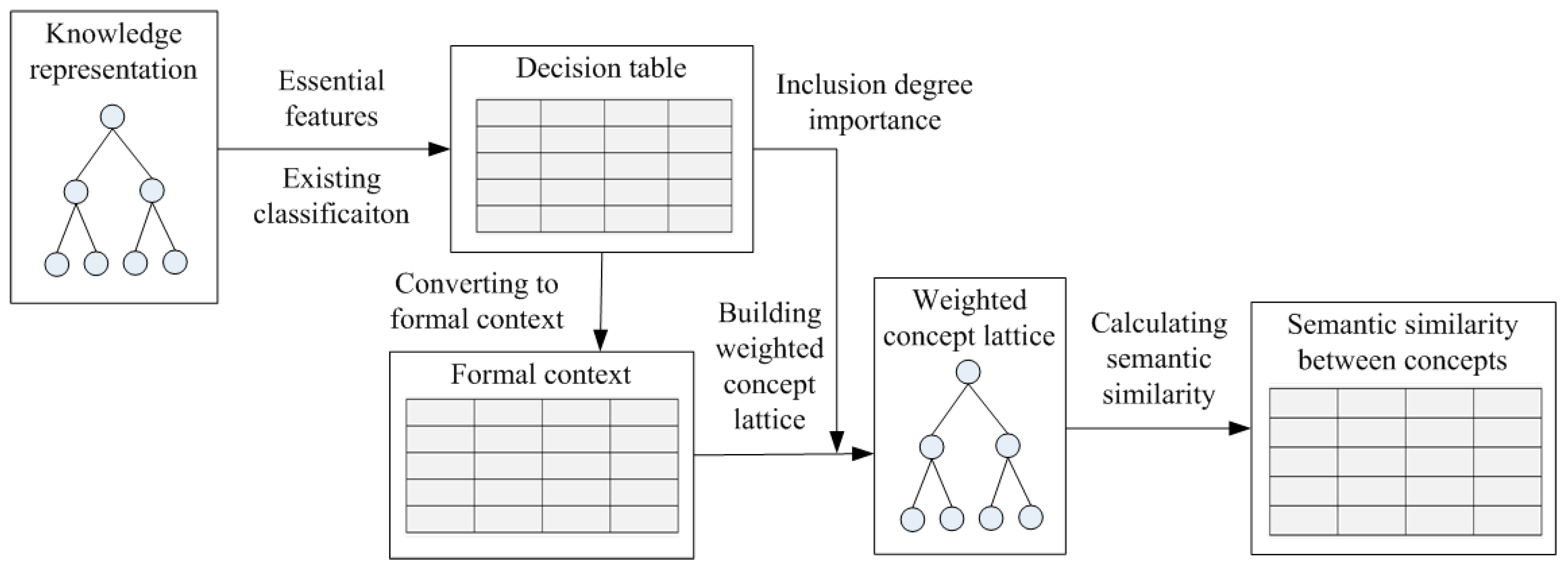
3. Weighted Concept Lattice

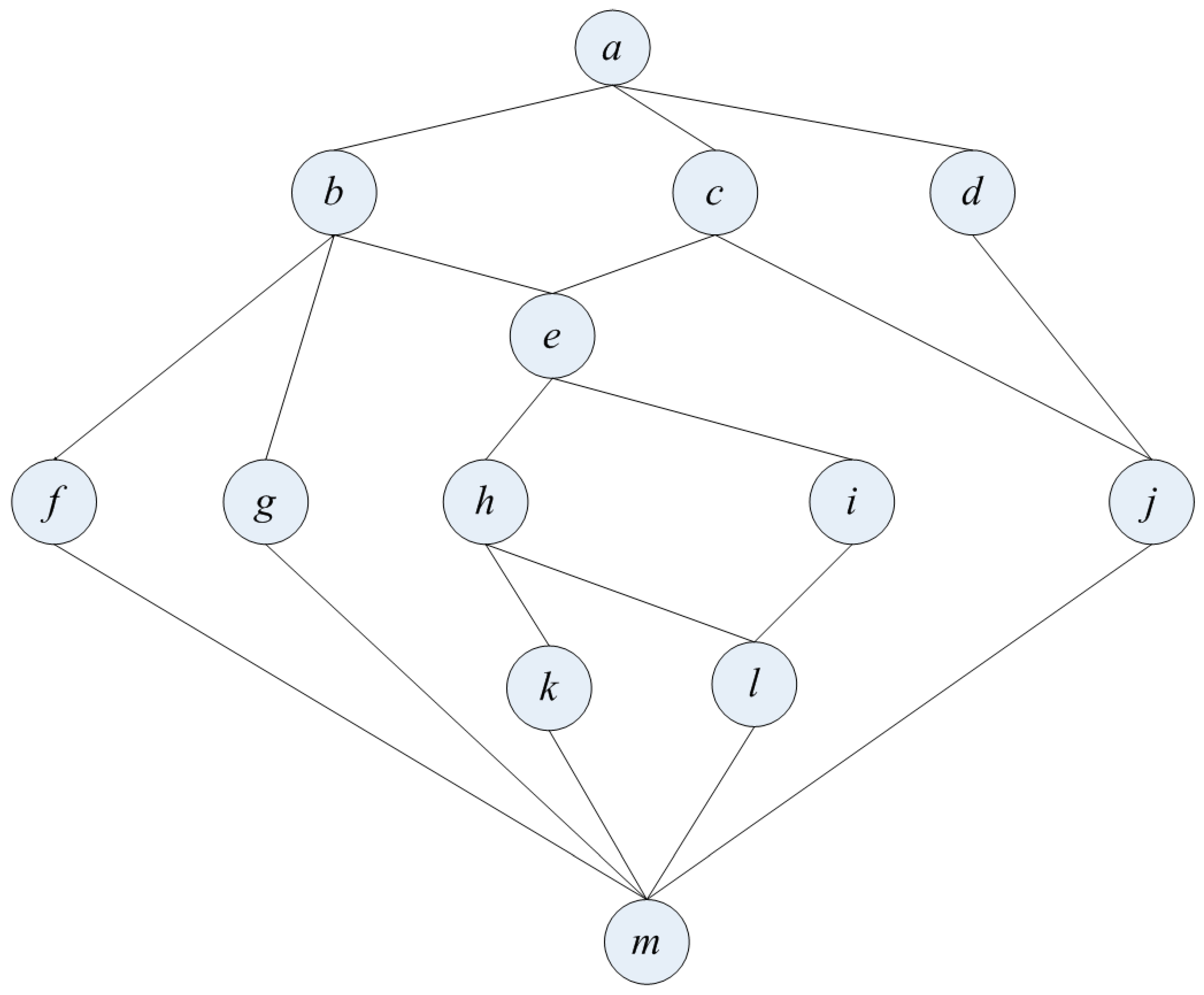
3.1. Knowledge Representation of the Feature Model

Discussing and establishing knowledge representation is not the main focus of this present paper. However, in order to make the discussion and demonstration clearer and more convenient, we first introduce the dataset, which will be used as the sample data in Section 5.

Ontology, defined as ‘a formal specification of a shared conceptualization’ [36], is considered to be an effective tool for specifically representing knowledge in various studies [37,38]. In geographic information science (GIScience), a number of scholars have tried to define essential properties of geo-ontologies and try to extract these properties from the definitions or descriptions of the geo-concepts’ categories and specifications [39,40]. Referring to a previous study [35], we extracted the essential properties of geo-ontologies (representing geo-concepts) based on geo-categories from GB/T 13923-2006 (specifications for feature classification and codes of fundamental geographic information) and definitions of these geo-categories from GB/T 20258.1-2007 (data dictionary for fundamental geographic information features). Partial inland hydrological concepts and their essential properties are presented in

Table 1. Geo-concepts with attributes table.

Concept	Material	Cause	Spatial Morphology	Spatial Location	Time	Material State	Function
lake	a	c	f	h	j	$\varnothing$	o
pond	a	d	f	h	j	$\varnothing$	o
seasonal lake	a	c	f	h	k	$\varnothing$	o
ground river	a	c	e	h	j	l	m
seasonal river	a	c	e	h	k	l	m
reservoir	a	d	f	h	$\varnothing$	$\varnothing$	(n, o)
spillway	a	d	e	i	$\varnothing$	$\varnothing$	n
dike	b	d	g	h	$\varnothing$	$\varnothing$	n

Note: Each letter from ‘a’ to ‘o’ represents the attributes in Table 2, while $\varnothing$ indicates that the object does not contain the attribute. As the object ‘reservoir’ includes two ‘function’ values (n and o), we represent its ‘function’ with ‘(n, o)’ which is a new value of the ‘function’ property.

.

3.2. Combined Weight of Attribute

Determining the weights of conceptual features is the key to measuring semantic similarity based on the feature model. In this paper, we represent conceptual features with properties or attributes. In the decision table, we use the property to refer to features. In the formal context and weighted concept lattices, a feature is represented as the attribute, which is the value of a specific property. For example, in Table 1, the geo-concept lake has the attribute of water, which is the value of its property material in

Table 2. Comparison table between attributes and identifiers.

Identifier	a	b	c	d	e	f
Attribute	material/	material/	cause/	cause/	spatial morphology/	spatial morphology/
	water	soil or stone	nature	artificial	long strip slot	depressions
Identifier	g	h	i	j	k	l
Attribute	spatial morphology/	spatial location/	spatial location/	time/	time/	material state/
	buildings	on the earth	underground	perennial	seasonal	flow
Identifier	m	n	o
Attribute	function/	function/	function/
	shipping	prevent flood	store water

. The weight of an attribute is computed via merging two factors that have mutually independent influences in our proposal. The first factor is the inclusion degree importance, which represents the degree to which the attribute impacts existing conceptual classification knowledge. We introduce information entropy as the other factor, which represents the average information of the weight of concepts comprising an attribute. The combination of these two influencing factors on an attribute, which is also known as its combined weight, represents the degree to which this attribute influences the semantic understanding of the concept.

3.2.1. Inclusion Degree Importance of a Property

In order to calculate the inclusion degree importance of a property, we first introduce the property importance from rough set theory. For more basic knowledge about the rough set, we refer readers to a previous study [41].

Definition 1.

An information system can be denoted as $S=(U,A,V,f)$, in which U is a non-empty and finite set of objects called the universe; A is a non-empty and finite set of attributes; $V={\bigcup }_{a\in A}{V}_a$, while $V_a$ is the domain of $a$; $f:U\times A\to V$ is an information function which assigns an information value to each property of each object, denoting $\forall a\in A, x\in U, f(x, a)\in V_a$. In particular, let $A=C\cup D$, where C is the set of condition attributes and D is the set of decision properties. If $C\cap D=\varnothing$, S is called a decision table.

For example,

Table 3. Decision table.

Concept	Material	Cause	Spatial Morphology	Spatial Location	Time	Material State	Function	Category
lake	a	c	f	h	j	$\varnothing$	o	230,000
pond	a	d	f	h	j	$\varnothing$	o	230,000
seasonal lake	a	c	f	h	k	$\varnothing$	o	230,000
ground river	a	c	e	h	j	l	m	210,000
seasonal river	a	c	e	h	k	l	m	210,000
reservoir	a	d	f	h	$\varnothing$	$\varnothing$	(n, o)	240,000
spillway	a	d	e	i	$\varnothing$	$\varnothing$	n	240,000
dike	b	d	g	h	$\varnothing$	$\varnothing$	n	270,000

Note: Each letter from ‘a’ to ‘o’ represents the same meaning as in Table 2, while ∅ indicates that the object does not contain the attribute. The value of field ‘category’ is the classification code of the super-category of the objects, which is the decision attribute in the decision table. As the object ‘reservoir’ includes two ‘function’ values (n and o) in the formal context (Table 1), we represent its ‘function’ with ‘(n, o)’ which is a new value of the ‘function’ property in the decision table.

is an information system, in which $U$ includes lake, pond, seasonal lake, ground river, seasonal river, reservoir, spillway and dike; and $A$ includes material, cause, spatial morphology, spatial location, time, material state, function and category. At the same time, it is a decision table if the attribute ‘category’ is considered as the decision property.

Definition 2.

Let $S=(U,A,V,f)$ be an information system, with each non-empty subset $B\subseteq A$. This determines an indiscernibility relation as follows:

$$ind(B)=\{(x,y)\in U\times U | \forall a\in B, f(x,a)=f(y,a)$$

(1)

Obviously, $ind(B)$ determines a partition of $U$ denoted as $U/ind(B)$ (for short $U/B$), which is also called a quotient set of $U$:

$$U/B=\{{[x]}_B | x\in U\}$$

(2)

where ${[x]}_B$ is the equivalence class determined by x with regards to B:

$${[x]}_B=\{y\in U | (x,y)\in ind(B)\}.$$

(3)

For example, in Table 3, $/\{material\}=\{\{lake,pond,seasonallake,groundriver,seasonalriver,reservoir,spillway\},\{dike\}\}$, and $U/\{material,cause\}=\{\{lake,seasonallake,groundriver,seasonalriver\},\{pond,reservoir,spillway\},\{dike\}\}$.

Definition 3.

Let $S=(U,C\cup D,V,f)$ be a decision table, where $X\subseteq U, B\subseteq C\cup D$, $\underset{\_}{BX}$ and $\overline{BX}$ denote B-lower and B-upper approximations of X, respectively:

$$\underset{\_}{BX}=\{x\in U | {[x]}_B\subseteq X\}$$

(4)

$$\overline{BX}=\{x\in U | {[x]}_B\cap X=\varnothing \}$$

(5)

For example, in Table 3, let $B=\{cause\}$ and $X=\{lake,pond,seasonallake,groundriver,seasonalriver\}$, thus, $\underset{\_}{BX}=\{lake,pond,seasonallake,seasonalriver\}$ and $\overline{BX}=\{lake,pond,seasonallake,groundriver,seasonalriver,reservoir,spillway,dike\}$.

Definition 4.

Let $S=(U,C\cup D,V,f)$ be a decision table and $B\subseteq C$, $PO{S}_B(D)$ is called the positive region of the partition $U/D$ with respect of B:

$$PO{S}_B(D)={\displaystyle \bigcup }_{X\in U/D}\underset{\_}{BX}$$

(6)

For example, in Table 3, let $B=\{material\}$ and $D=\{category\}$, thus, $PO{S}_B(D)=\{dike\}$.

Definition 5.

Let $S=(U,C\cup D,V,f)$ be a decision table and $B\subseteq C$, $si{g}_{CD}(B)$ denotes the importance of $U/D$ with respect to B:

$$si{g}_{CD}(B)={\gamma }_C(D)-{\gamma }_{C-B}(D)$$

(7)

In particular, let $B=\{a\}$, the importance of $U/D$ with respect to $a$ is:

$$si{g}_{CD}(a)={\gamma }_C(D)-{\gamma }_{C-\{a\}}(D)$$

(8)

where ${\gamma }_C(D)=|PO{S}_C(D)|/|U|$.

For example, in Table 3, $|PO{S}_C(D)|=8$ and $|U|=8$, thus, ${\gamma }_C(D)=1$. ${\gamma }_{C-\{material\}}(D)=\left|PO{S}_{C-\{material\}}(D)\right|/|U|=8/8=1$, thus, $si{g}_{CD}(material)=0$.

A decision table is constructed in our work via adding decision properties into the object-attribute table. For instance, a decision table (Table 3) is built by inserting classification knowledge of concepts into Table 1. Generally, the decision properties are represented by the existing classification knowledge, such as industry standards or specifications, expert opinions etc. The existing classification knowledge of concepts reflects a specific application context to a great extent, which involves the general understanding of a specific domain within a relatively long period of time. Therefore, the importance weight of a condition property, which is inversely calculated from decision properties, reflects the degree of influence of this condition property on the semantic understanding of the concept.

Although the importance of a condition property could quantify the weight of influence it has on the semantic understanding of the concept, this parameter will lose its function of distinguishing the importance of different properties when unnecessary properties exist in the decision table or when the decision table has more than one reduction result. Therefore, we introduced the inclusion degree proposed in a previous study [42], which is a solution to this problem.

Given two sets, X and Y, we define a function as follows:

$$con(X/Y)=\{\begin{array}{c}0,X\not\subset Y;\\ 1,X\subseteq Y;\end{array}$$

(9)

Definition 6.

Let $S=(U,C\cup D,V,f)$ be a decision table and $A_1,A_2\subseteq C\cup D$. Therefore, $U/ A_1=\{X_1, X_2\dots X_n\}$ and $U/A_2=\{Y_1, Y_2\dots Y_m\}$ are partitions of $U$, respectively. We denote $CON(A_1/A_2)$ as the inclusion degree of $U/A_2$ to $U/A_1$:

$$CON(A_1/A_2)={\displaystyle \sum }_{\begin{array}{c}0\le i\le n\\ 0\le j\le m\end{array}}con\left(\frac{X_i}{Y_j}\right)$$

(10)

Obviously, $0\le CON(A_1/A_2)\le n$, especially if ${\mathrm{A}}_1$ is smaller than ${\mathrm{A}}_2$. This means that $\forall X_i, \exists Y_j$ makes $X_i\subseteq Y_j$ with $CON(A_1/A_2)$ have the maximum value of n.

For example, in Table 3, $U/\{material\}=\{\{lake, pond, seasonal lake, ground river, seasonal river, reservoir, spillway\}, \{dike\}\}$ and $U/\{category\}=\{\{lake, pond, seasonal lake\}, \{ground river, seasonal river\}, \{reservoir, spillway\},\{dike\}\}$, thus $CON(\{material\}/\{category\})=1$ and $CON(\{category\}/\{material\})=4$.

Definition 7.

Let $S=(U,C\cup D,V,f)$ be a decision table, with property $a\in C$. $SI{G}_{CD}(a)$ denotes the property importance of the inclusion degree:

$$SI{G}_{CD}(a)=({|U|}^{2}si{g}_{CD}(a)+|U|p_a-q_a+1)/({|U|}^2+|U|+1)$$

(11)

where

$$p_a=(|PO{S}_a(D)|+CON(a/D)/|U|)/(|U|+1)$$

$$q_a=(|PO{S}_D(a)|+CON(D/a)/|U|)/(|U|+1)$$

$p_a$ and $q_a$ represent the influence of the positive region and the inclusion degree on the property importance, respectively.

For example, in Table 3, $p_{material}=(1+1/8)/(8+1)=0.125$ and $q_{material}=(8+4/8)/(8+1)=0.944$, thus $SI{G}_{CD}(material)=(0+8\times 0.125-0.944+1)/(64+8+1)=0.0145$.

3.2.2. Formal Context

Before discussing the information entropy of attributes, we introduce the formal context from formal concept analysis (FCA).

Definition 8.

In FCA, a formal context is described by a triple $K=(G,M,I)$, where G and M represent two non-empty sets of objects (called extent) and attributes (called intent), respectively, while I is a subset of the Cartesian product of G and M ($I\subseteq G\times M$). When $g\in G$ and $m\in M$, it means that object g has the attribute m, and that attribute m belongs to object g if gIm.

For example,

Table 4. A formal context converted from the decision table.

SN	Object	a	b	c	d	e	f	g	h	i	j	k	l	m	n	o
$s_1$	lake	*		*			*		*		*					*
$s_2$	pond	*			*		*		*		*					*
$s_3$	seasonal lake	*		*			*		*			*				*
$s_4$	ground river	*		*		*			*		*		*	*
$s_5$	seasonal river	*		*		*			*			*	*	*
$s_6$	reservoir	*			*		*		*						*	*
$s_7$	spillway	*			*	*				*					*
$s_8$	dike		*		*			*	*						*

Note: Each letter from ‘a’ to ‘o’ represents attributes in Table 2, while * represents a satisfied criterion.

is a formal context, in which $G=\{s_1,s_2,s_3,s_4,s_5,s_6,s_7,s_8\}$ and $M=\{a,b,\mathrm{c},d,e,\mathrm{f},\mathrm{g},\mathrm{h},\mathrm{i},\mathrm{j},\mathrm{k},\mathrm{l},\mathrm{m},\mathrm{n},\mathrm{o}\}$.

According to Definition 8, we can construct a formal context that is converted from the decision table (excluding decision properties) in which the value of properties is transformed into attributes of the formal context. As presented in Table 4, the attribute that holds for a specific concept is marked with ‘*’. Based on the formal context, which is also an object-attribute table, we introduce the information entropy to quantify the weights of the attributes.

3.2.3. Information Entropy of Attributes

Definition 9.

Let $K=(G,M,I)$ be a formal context, where $G=\{g_1,g_2,\dots ,g_n\}$ and $M=\{m_1,m_2,\dots ,m_k\}$. Thus, $p(m/g)$ denotes the probability of object $g$ possessing the corresponding attribute $m$, while $E(m)$ representing information entropy is the average information of attribute $m$ provided by $G$, the set of objects. Following this, we can compute $E(m_j)(1\le j\le k)$ according to the following formula:

$$E\left(m_j\right)=-{\displaystyle \sum }_{i=1}^{n}p(m_j/g_i)lo{g}_{2}p(m_j/g_i)$$

(12)

Before the combined weight of the attribute is calculated, we introduce the inclusion degree importance of the attribute based on the inclusion degree importance of the properties, Equation (11).

For example, in Table 4, $E(a)=-{{\displaystyle \sum }}_{i=1}^1(7/8)\times lo{g}_2(7/8)=0.169$.

Definition 10.

Let $K=(G,M,I)$ be a formal context, which is converted from the conditional properties of the decision table $S$, where $G=\{g_1,g_2,\dots ,g_n\}$ and $M=\{m_1,m_2,\dots ,m_k\}$, $SIG\left(m_j\right)$ denotes the importance of the inclusion degree of attribute $m_j$ based on decision table $S$:

$$SIG\left(m_j\right)=SI{G}_{CD}\left(\left[m_j\right]\right)/|\left[m_j\right]|$$

(13)

where $\left[m_j\right]\in C$ represents one of the conditional properties in decision table $S$, its possible value is $m_j$, and $|\left[m_j\right]|$ is the number of nonempty value of $\left[m_j\right]$.

For example, according to the decision table (Table 3), $[a]=[b]=material$, thus $|[a]|=2$. Therefore, $SIG(a)=SI{G}_{CD}(material)/|material|=0.0145/2=0.0072$.

Thus, we can calculate the combined weight of attributes using the information entropy of attributes, Equation (12), and the inclusion-degree importance of the attributes, Equation (13).

Definition 11.

Let $K=(G,M,I)$ be a formal context, where $G=\{g_1,g_2,\dots ,g_n\}$ and $M=\{m_1,m_2,\dots ,m_k\}$, and $w_{m_j}(1\le j\le k)$ is the combined weight of inclusion-degree importance and information entropy of attribute $m_j$. Following this, we define $K_W=(G,M,I,W)$ as a weighted formal context generated from $K$, where $w_{m_j}\in W$.

$$w_{m_j}=SIG\left(m_j\right)\ast E\left(m_j\right)/({\displaystyle \sum }_{i=1}^{k}SIG\left(m_j\right)\ast E\left(m_j\right))$$

(14)

where $E\left(m_j\right)$ and $SIG\left(m_j\right)$ are calculated via Equations (12) and (13) respectively.

For example, $w_a=SIG(a)\ast E(a)/({{\displaystyle \sum }}_{i=1}^{k}SIG\left(m_j\right)\ast E\left(m_j\right))=0.0153$. The combined weights of all attributes are listed in Section 5.

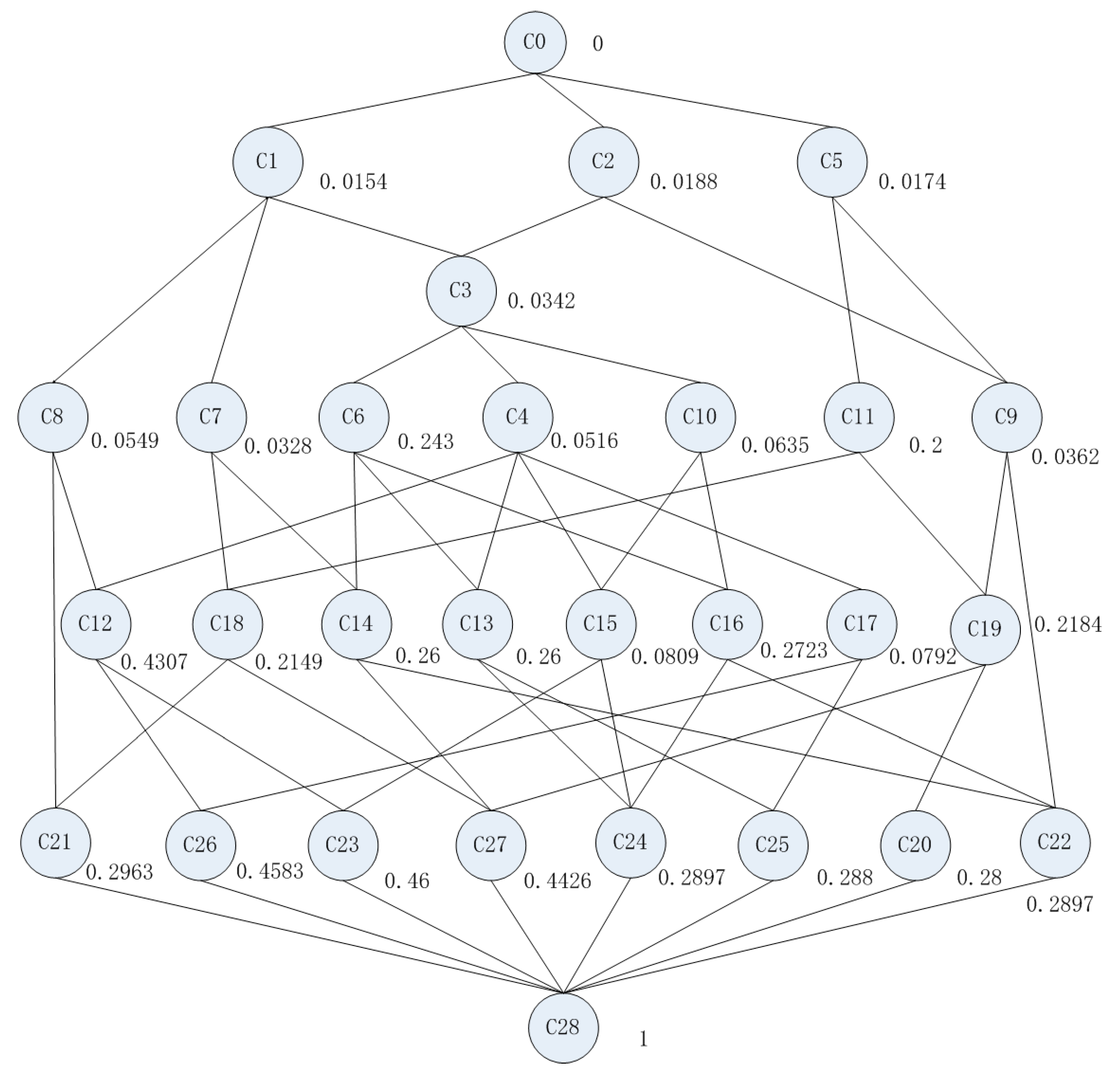
3.3. Construction of the Weighted Concept Lattice

From Definition 11, the weighted formal context is defined by assigning combined weight to each attribute of the formal context. Following this, based on the theory of formal concept analysis, we define the weighted concept lattice from the weighted formal context. We refer readers to [32] to obtain more basic knowledge about the concept lattice in FCA.

Definition 12.

Let $K=(G,M,I)$ be a formal context, with two sets, $A\subseteq G$ and $B\subseteq M$. If every element (object) in A contains all of the attributes in B and every element (attribute) in B belongs to all of the objects in A, respectively, the following operations are denoted:

$$A=B^{\prime }=\{a\in G | b\in B, aIb\}$$

(15)

$$B=A^{\prime }=\{b\in M | a\in A, aIb\}$$

(16)

then, the tuple $(A,B)$ is a formal concept of $K$, if $A=B^{\prime }$ and $B=A^{\prime }$.

Given that $({\mathrm{A}}_1,{\mathrm{B}}_1)$ and $({\mathrm{A}}_2,{\mathrm{B}}_2)$ are two formal concepts of $\mathrm{K}$, there is a partial order relation ($\le$) between them if they satisfy the following condition:

$$({\mathrm{A}}_1,{\mathrm{B}}_1)\le ({\mathrm{A}}_2,{\mathrm{B}}_2)\iff {\mathrm{A}}_1\subseteq {\mathrm{A}}_2\iff {\mathrm{B}}_2\subseteq {\mathrm{B}}_1$$

(17)

All formal concepts created from the formal context $K=(G,M,I)$ are able to establish a hierarchical structure based on the partial order relation ($\le$) between concepts, named the concept lattice, which is denoted as $(\mathsf{ℒ}(\mathrm{G},\mathrm{M},\mathrm{I}),\le )$ or $(\mathsf{ℒ},\le )$. A concept lattice is a complete lattice.

For example, according to Definition 12, the tuple $(\{s_6,s_8\},\{d,h,n\})$ is a formal concept generated from the formal context (Table 4) and $(\{s_8\},\{b,d,g,h,n\})$ is a formal concept too. Also, these two formal concepts have a partial order relation which is denoted as $(\{s_8\},\{b,d,g,h,n\})\le (\{s_6,s_8\},\{d,h,n\})$.

Definition 13.

Let $K=(G,M,I)$ be a formal context, $K_W=(G,M,I,W)$ is the weighted formal context generated from $K$ and $(ℒ(G,M,I),\le )$ is the concept lattice established from $K$. Following this, we define $({ℒ}_W(G,M,I,W),\le )$ as the weighted concept lattice of $K_W$. $({ℒ}_W(G,M,I,W),\le )$ has the same elements of $(G,M,I)$ and the same structure with $(ℒ(G,M,I),\le )$, while the each attribute in $({ℒ}_W(G,M,I,W),\le )$ is assigned with the different weight.

Definition 14.

Let $(ℒ(G,M,I),\le )$ and $({ℒ}_W(G,M,I,W),\le )$ be a concept lattice and weighted concept lattice respectively. Given that $(A,B)$ is a formal concept in $(ℒ,\le )$, we define $(A,B,w)$ as a weighted formal concept of $({ℒ}_W,\le )$, in which $w$ denotes the sum of weights of attributes that belong to its intent $B$.

$$w={\displaystyle \sum }_{m\in B}{w}_m,$$

(18)

According to Equation (14), the combined weight of each attribute can be calculated. Following this, we use Equation (18) to assign weight to each formal concept. For example, let $A=(\{s_8\},\{b,d,g,h,n\})$, $A$ is a formal concept, and the weight of $A$ is the sum of weights of $\{b,d,g,h,n\}$; thus $w={{\displaystyle \sum }}_{m\in \{b,d,g,h,n\}}{w}_m=0.2184$. Therefore, $(\{s_8\},\{b,d,g,h,n\},0.2184)$ is a weighted formal concept.

4. Semantic Similarity Measurement

With Definitions 13 and 14, we construct a weighted concept lattice based on a weighted formal context. Every vertex in this weighted concept lattice represents a weighted formal concept, the weight of which is calculated using Equation (18). In this section, a novel approach with detailed procedures is introduced to measure the semantic similarity between different weighted formal concepts in the weighted concept lattice. In particular, the formal concepts that include only one original geo-concept in their extent can be regarded as the original geo-concepts themselves. Therefore, the semantic similarities between these weighted formal concepts are considered to be those of the original geo-concepts. Meanwhile, the super-categories of these original geo-concepts can be represented by the weighted concepts that possess the same attributes in the lattice. Therefore, the concepts for comparison are not only restricted to the original geo-concepts but extended to their super-categories.

Before measuring the semantic similarity of the weighted concepts in the weighted concept lattice, we first introduce the relative hierarchical depth of concepts in the concept lattice to quantify the degree of impact that the concept hierarchy has on the semantic differences.

4.1. Relative Hierarchical Depth

Definition 15.

Let $(ℒ,\le )$ be a concept lattice. Given ${ℒ}^{\prime }\subseteq ℒ$ is a subset of $ℒ$, we denote $sup({ℒ}^{\prime })$ as the supremum of the subset ${ℒ}^{\prime }$, respectively. As the concept lattice $(ℒ,\le )$ is a complete lattice, $sup({ℒ}^{\prime })\in ℒ$ and $sup({ℒ}^{\prime })\ne \varnothing$. In particular, if ${ℒ}^{\prime }$ contains only two elements(${ℒ}^{\prime }=\{a,b\}$), we denote $sup(a,b)$ as the supremum of concept $a$ and $b$.

For example, in the concept lattice $(\mathsf{ℒ},\le )$ (Figure 2), $sup(g,h)=sup(h,g)=b$.

Definition 16.

Let $(ℒ,\le )$ be a concept lattice. We define $a$ and $c$ as two formal concepts, given that $a,c\in ℒ$ and $a\le c$. Thus, we denote $dis (a,c)$ as the shortest distance from $a$ to $c$ in the lattice, which means the least count of edges between vertices that connect vertices $a$ and $c$ in the lattice. Furthermore, we define $dis (a,a)=0$.

For instance, in the concept lattice $(\mathsf{ℒ},\le )$ (Figure 2), as $k\le c$ in the lattice, we can calculate $dis (k,c)=3$ and $dis (j,c)=1$. However, because $c\nleqq k$, $dis (c,k)$ is not defined. Thus, $dis (i,j)$ and $dis (j,i)$ are also not defined. The shortest distance is only defined from a sub-concept to its super-concept or itself.

In the network model, the distance between vertices representing concepts is usually an important indicator that reflects their semantic similarity. In the transformation model [43], the steps through which one concept is transformed to another are also regarded as a specific type of ‘distance’. This particular ‘distance’ is also used to represent the semantic similarity between these two concepts. Similarly, the shortest distance from a sub-concept to its super-concept in Definition 16 possesses such a function. However, this parameter, the shortest distance of $\mathrm{dis}$, focuses on representing the degree of differences between the sub-concept and one of its super-concepts. In the concept lattice, the intent of the super-concept is always a proper subset of the intent of its sub-concept. Therefore, the sub-concepts have the same general characteristics as the super-concept in the concept lattice. Thus, the shortest distance reflects the degree of differences between the sets of characteristics of a sub-concept and its specific super-concept. A longer shortest distance indicates a larger degree of differences between these two concepts. For instance, in the concept lattice $(\mathsf{ℒ},\le )$ (Figure 2), the concepts $i$ and $j$ have the same super-concept $c$, but $dis (i,c)=2$ while $\mathrm{dis}(j,c)=1$. Therefore, the concept $i$ has a larger degree of difference from $c$ than the concept $j$ does.

Definition 17.

Let $(ℒ,\le )$ be a concept lattice. We denote $a$ and $b$ are two formal concepts. Given that $a,c\in ℒ$ and $a\le c$, we denote $rhd (a,c)$ as the relative hierarchical depth of $a$ to $c$ in the concept lattice. $rhd (a,c)$ is defined as follow:

$$rhd (a,c)=dis (a,c)/(dis (a,c)+dis (c,sup(ℒ)))$$

(19)

where $sup (ℒ)$ is the supremum of the $ℒ$ that is actually the largest element of the lattice $(ℒ,\le )$. Furthermore, we define $rhd (a,a)=0$.

For instance, in the concept lattice $(\mathsf{ℒ},\le )$ (Figure 2), as $k\le c$ in the lattice, we can $\mathrm{calculate}rhd (k,c)=3/(3+1)=3/4$ and $dis (j,c)=1/(1+1)=1/2$. However, because $c\nleqq k$, $dis (c,k)$ is not defined. Thus, $dis (i,j)$ and $dis (j,i)$ are not defined too. The relative hierarchical depth is only defined from a sub-concept to its super-concept or itself.

Although the shortest distance proposed in Definition 16 is able to reflect the different degree between concepts having partial relations in the concept lattice, this parameter is unable to distinguish the hierarchical differences of concepts. For instance, in the concept lattice $(\mathsf{ℒ},\le )$ (Figure 2), $dis (k,h)=dis (e,c)=1$. However, it is intuitively clear that the degrees between $k,h$ and $e,c$ are quite different. Therefore, in Definition 17, we introduce the relative hierarchical depth taking the impact of different hierarchies on the shortest distance between concepts into account. Thus, $rhd (k,h)=1/4$ and $rhd (e,c)=1/2$, which demonstrates that a lower hierarchy of the concept results in a smaller impact on the degree of difference.

4.2. Semantic Similarity Model

Proposed by Tversky, the contrast and ratio models (Equations (20) and (21)) are the prototypes for most approaches based on the feature model. These algorithm models have been widely used and developed into many new versions. For example, the MDSM extended it by distinguishing different types of features including parts, attributes, and functions [8].

$$S(a,b)=\theta \ast f(A\cap B)+\alpha \ast f(A-B)+\beta \ast f(B-A)$$

(20)

$$S(a,b)=f(A\cap B)/(f(A\cap B)+\alpha \ast f(A-B)+\beta \ast f(B-A))$$

(21)

In our work, we first introduce the absolute semantic similarity between concepts in the weighted concept lattice based on the contrast model, Equation (20). Following this, we propose a relative semantic similarity of concepts that is able to reflect and explain the cognitive cause of an asymmetric property of semantic similarity to some extent.

Definition 18.

Let $(ℒ(G,M,I,W),\le )$ be a weighted concept lattice, Furthermore, $a=(A_1,B_1)$ and $b=(A_2,B_2)$ are two formal concepts. Given $a,b\in ℒ$ and $c=sup (a,b)=(A_3,B_3)$ we denote $sim (a,b)$ as the relative semantic similarity between concepts $a$ and $b$, which is defined as follow:

$$sim(a,b)={\displaystyle \sum }_{m_1\in B_3}{w}_{m_1}-rhd(a,c)\ast {\displaystyle \sum }_{m_2\in B_1-B_3}{w}_{m_2}-rhd(b,c)\ast {\displaystyle \sum }_{m_3\in B_2-B_3}{w}_{m_3},$$

(22)

where $rhd (a,c)$ and $rhd (b,c)$ are the relative hierarchical depths of concepts $a$ and $b$ to $c$.

For example, let the lattice represented by Figure 2 be a weighted concept lattice, and the concept $k=(A_1,\{m_1,m_2,m_3,m_4\})$ and $j=(A_2,\{m_1,m_5\})$. We assume that $w_{m_1}=0.6$, $w_{m_2}=0.2$, $w_{m_3}=0.1$, $w_{m_4}=0.3$ and $w_{m_5}=0.2$ according to Equation (14). Thus, $(k,j)=sim(j,k)=0.6-(3/4)\times (0.2+0.1+0.3)-(1/2)\times 0.2=0.05$.

In Equation (22), we compare the commonalities and differences of weighted attributes between concepts based on the contrast model. However, in this formula of the absolute semantic similarity computation, the combined weighted difference of attributes and hierarchical depth difference of concepts are taken into account.

From Equation (22), the absolute semantic similarity has a symmetrical property and thus $sim (a,b)=sim (b,a)$. However, according to Tversky’s famous statement that similarity or dissimilarity is judged depending on the prominence or relative salience of concepts, the semantic similarity holds an asymmetrical property. Therefore, we introduce the relative semantic similarity, which is measured by the proportion of absolute semantic similarity in the semantic intent of the concept.

Definition 19.

Let $(ℒ(G,M,I,W),\le )$ be a weighted concept lattice, while $a$ and $b$ are two formal concepts. Given $a,b\in ℒ$, we then denote $SIM(a,b)$ as the relative semantic similarity, or semantic similarity, of concepts $a$ to $b$, which is defined as follows:

$$SIM(a,b)=2^{sim(a,b)/sim(a,a)-1}$$

(23)

where $sim (a,b)=sim (b,a)$ is the absolute semantic similarity between concepts $a$ to $b$, and $sim (a,a)$ is the absolute semantic similarity of concept $a$ to itself.

We set the same assumptions as in the previous example; thus $sim (k,j)=sim (j,k)=0.05$. Using Equation (22), we can calculate $sim (k,k)=1.2$ and $sim (j,j)=0.7$. Therefore, $SIM (k,j)=0.515$ and $SIM (j,k)=0.525$.

In Equation (23), $sim (a,b)/sim (a,a)$ represents the relative proportion of the absolute semantic similarity in the concept $\mathrm{a}$. The range of this parameter is from negative infinity to one, which means that $sim (a,b)/sim (a,a)\in (-\infty ,1]$. Following this, we introduce the exponential function to normalize it, and define the normalized result as the relative semantic similarity or semantic similarity of concepts $\mathrm{a}$ to $\mathrm{b}$. From Definition 19, we know that this has an asymmetrical property with a range of 0–1 ($SIM (a,b)\in (0,1]$). In particular, if $SIM (a,b)=1/2$, it means that the similarity and dissimilarity between concepts $\mathrm{a}$ to $\mathrm{b}$ are approximately equal. In this case, $SIM (a,b)=SIM(b,a)=1/2$.

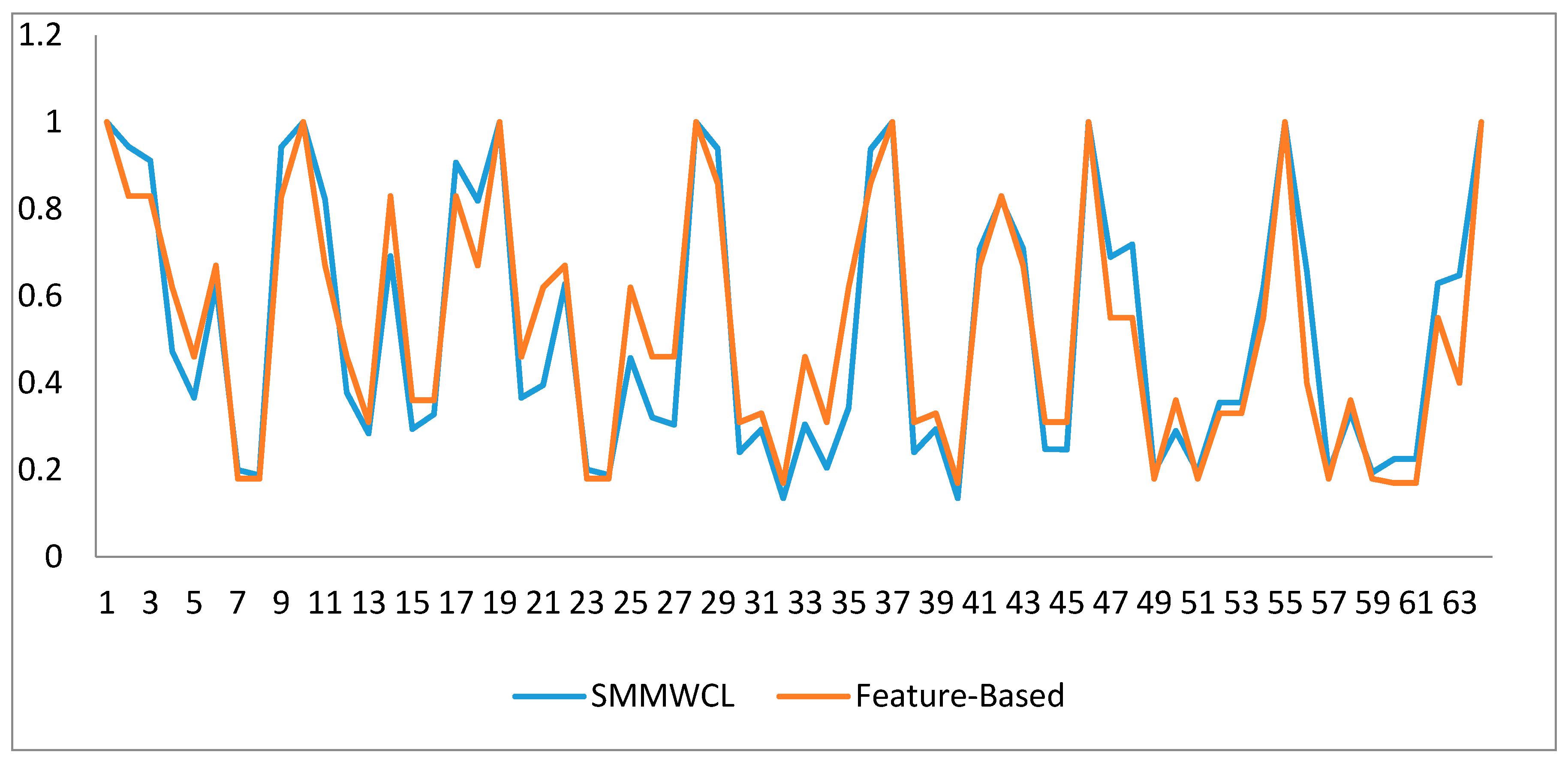
5. Case Study and Discussion

In Section 3.2, by extracting the essential properties of partial geo-concepts from their definitions in GB/T 20258.1-2007, we build the object-properties table (Table 1) of geo-concepts. Obtaining the classification of these geo-concepts from GB/T 13923-2006 as the decision property, we subsequently add this decision property into Table 1 in order to establish a decision table (Table 3). Finally, a formal context (Table 4) is built by converting the decision table (Table 3).

Using Equation (11) in Section 3.2.1, the inclusion-degree weight of each property in the decision table is calculated, with the results shown in

Table 5. Weights of properties in the decision table.

Inclusion Degree	Material	Cause	Spatial Morphology	Spatial Location	Time	Material State	Function
SIG (property)	0.0145	0.0055	0.0177	0.0177	0.0875	0.0266	0.0816

. Following this, the information entropy and inclusion degree of each attribute are calculated via Equations (12) and (13) respectively. Next, we substitute these parameters in Equation (14) to obtain the combined weight of each attribute. The results of the combined weights of attributes are shown in

Table 6. Attribute weight value of the formal context.

Attribute	p (x)	E (x)	SIG (x)	w (x)
a	0.875	0.169	0.0072	0.0153
b	0.125	0.375	0.0072	0.0342
c	0.500	0.500	0.0028	0.0174
d	0.500	0.500	0.0028	0.0174
e	0.375	0.531	0.0059	0.0395
f	0.500	0.500	0.0059	0.0372
g	0.125	0.375	0.0059	0.0279
h	0.875	0.169	0.0089	0.0188
i	0.125	0.375	0.0089	0.0419
j	0.375	0.531	0.0044	0.0293
k	0.250	0.500	0.0044	0.0276
l	0.250	0.500	0.0266	0.168
m	0.250	0.500	0.0272	0.1716
n	0.375	0.531	0.0272	0.1821
o	0.500	0.500	0.0272	0.1716

after normalization.

We calculate all formal concepts from the formal context of Table 4. After calculating the weight of each formal concept based on Equation (18), all weighted formal concepts are demonstrated as follows.

$$\begin{gathered} {\mathrm{C}}_0=(\{{\mathrm{s}}_1,{\mathrm{s}}_2,{\mathrm{s}}_3,{\mathrm{s}}_4,{\mathrm{s}}_5,{\mathrm{s}}_6,{\mathrm{s}}_7,{\mathrm{s}}_8\};\varnothing ;0); \\ {\mathrm{C}}_1=(\{{\mathrm{s}}_1,{\mathrm{s}}_2,{\mathrm{s}}_3,{\mathrm{s}}_4,{\mathrm{s}}_5,{\mathrm{s}}_6,{\mathrm{s}}_7\};\{\mathrm{a}\};0.0154); \\ {\mathrm{C}}_2=(\{{\mathrm{s}}_1,{\mathrm{s}}_2,{\mathrm{s}}_3,{\mathrm{s}}_4,{\mathrm{s}}_5,{\mathrm{s}}_6,{\mathrm{s}}_8\};\{\mathrm{h}\};0.0188); \\ {\mathrm{C}}_3=(\{{\mathrm{s}}_1,{\mathrm{s}}_2,{\mathrm{s}}_3,{\mathrm{s}}_4,{\mathrm{s}}_5,{\mathrm{s}}_6\};\{\mathrm{a},\mathrm{h}\};0.0342); \\ {\mathrm{C}}_4=(\{{\mathrm{s}}_1,{\mathrm{s}}_3,{\mathrm{s}}_4,{\mathrm{s}}_5\};\{\mathrm{a},\mathrm{c},\mathrm{h}\};0.0516); \\ {\mathrm{C}}_5=(\{{\mathrm{s}}_2,{\mathrm{s}}_6,{\mathrm{s}}_7,{\mathrm{s}}_8\};\{\mathrm{d}\};0.0174); \\ {\mathrm{C}}_6=(\{{\mathrm{s}}_1,{\mathrm{s}}_2,{\mathrm{s}}_3,{\mathrm{s}}_6\};\{\mathrm{a},\mathrm{f},\mathrm{h},\mathrm{o}\};0.243); \\ {\mathrm{C}}_7=(\{{\mathrm{s}}_2,{\mathrm{s}}_6,{\mathrm{s}}_7\};\{\mathrm{a},\mathrm{d}\};0.0328); \\ {\mathrm{C}}_8=(\{{\mathrm{s}}_4,{\mathrm{s}}_5,{\mathrm{s}}_7\};\{\mathrm{a},\mathrm{e}\};0.0549); \\ {\mathrm{C}}_9=(\{{\mathrm{s}}_2,{\mathrm{s}}_6,{\mathrm{s}}_8\};\{\mathrm{d},\mathrm{h}\};0.0362); \\ {\mathrm{C}}_{10}=(\{{\mathrm{s}}_1,{\mathrm{s}}_2,{\mathrm{s}}_4\};\{\mathrm{a},\mathrm{h},\mathrm{j}\};0.0635); \\ {\mathrm{C}}_{11}=(\{{\mathrm{s}}_6,{\mathrm{s}}_7,{\mathrm{s}}_8\};\{\mathrm{d},\mathrm{n}\};0.2); \\ {\mathrm{C}}_{12}=(\{{\mathrm{s}}_4,{\mathrm{s}}_5\};\{\mathrm{a},\mathrm{c},\mathrm{e},\mathrm{h},\mathrm{l},\mathrm{m}\};0.4307); \\ {\mathrm{C}}_{13}=(\{{\mathrm{s}}_1,{\mathrm{s}}_3\};\{\mathrm{a},\mathrm{c},\mathrm{f},\mathrm{h},\mathrm{o}\};0.26); \\ {\mathrm{C}}_{14}=(\{{\mathrm{s}}_2,{\mathrm{s}}_6\};\{\mathrm{a},\mathrm{d},\mathrm{f},\mathrm{h},\mathrm{o}\};0.26); \\ {\mathrm{C}}_{15}=(\{{\mathrm{s}}_1,{\mathrm{s}}_4\};\{\mathrm{a},\mathrm{c},\mathrm{h},\mathrm{j}\};0.0809); \\ {\mathrm{C}}_{16}=(\{{\mathrm{s}}_1,{\mathrm{s}}_2\};\{\mathrm{a},\mathrm{f},\mathrm{h},\mathrm{j},\mathrm{o}\};0.2723); \\ {\mathrm{C}}_{17}=(\{{\mathrm{s}}_3,{\mathrm{s}}_5\};\{\mathrm{a},\mathrm{c},\mathrm{h},\mathrm{k}\};0.0792); \\ {\mathrm{C}}_{18}=(\{{\mathrm{s}}_6,{\mathrm{s}}_7\};\{\mathrm{a},\mathrm{d},\mathrm{n}\};0.2149); \\ {\mathrm{C}}_{19}=(\{{\mathrm{s}}_6,{\mathrm{s}}_8\};\{\mathrm{d},\mathrm{h},\mathrm{n}\};0.2184); \\ {\mathrm{C}}_{20}=(\{{\mathrm{s}}_8\};\{\mathrm{b},\mathrm{d},\mathrm{g},\mathrm{h},\mathrm{n}\};0.28); \\ {\mathrm{C}}_{21}=(\{{\mathrm{s}}_7\};\{\mathrm{a},\mathrm{d},\mathrm{e},\mathrm{i},\mathrm{n}\};0.2963); \\ {\mathrm{C}}_{22}=(\{{\mathrm{s}}_2\};\{\mathrm{a},\mathrm{d},\mathrm{f},\mathrm{h},\mathrm{j},\mathrm{o}\};0.2897); \\ {\mathrm{C}}_{23}=(\{{\mathrm{s}}_4\};\{\mathrm{a},\mathrm{c},\mathrm{e},\mathrm{h},\mathrm{j},\mathrm{l},\mathrm{m}\};0.46); \\ {\mathrm{C}}_{24}=(\{{\mathrm{s}}_1\};\{\mathrm{a},\mathrm{c},\mathrm{f},\mathrm{h},\mathrm{j},\mathrm{o}\};0.2897); \\ {\mathrm{C}}_{25}=(\{{\mathrm{s}}_3\};\{\mathrm{a},\mathrm{c},\mathrm{f},\mathrm{h},\mathrm{k},\mathrm{o}\};0.288); \\ {\mathrm{C}}_{26}=(\{{\mathrm{s}}_5\};\{\mathrm{a},\mathrm{c},\mathrm{e},\mathrm{h},\mathrm{k},\mathrm{l},\mathrm{m}\};0.4583); \\ {\mathrm{C}}_{27}=(\{{\mathrm{s}}_6\};\{\mathrm{a},\mathrm{d},\mathrm{f},\mathrm{h},\mathrm{n},\mathrm{o}\};0.4426); \\ {\mathrm{C}}_{28}=(\varnothing ;\{\mathrm{a},\mathrm{b},\mathrm{c},\mathrm{e},\mathrm{f},\mathrm{g},\mathrm{h},\mathrm{i},\mathrm{j},\mathrm{k},\mathrm{l},\mathrm{m},\mathrm{n},\mathrm{o}\};1); \end{gathered}$$

All weighted formal concepts are used to establish a weighted concept lattice (Figure 3) via a partial order relation according to Definition 12. Noticing that each of the formal concepts ${\mathrm{C}}_{24}, {\mathrm{C}}_{22}, {\mathrm{C}}_{25}, {\mathrm{C}}_{23}, {\mathrm{C}}_{26}, {\mathrm{C}}_{27}, {\mathrm{C}}_{21}, {\mathrm{C}}_{20}$ includes only one original geo-concept in their extent, we use them to represent the original geo-concepts of ${\mathrm{s}}_{1-8}$. That means that the semantic similarities of formal concepts in the weighted concept lattice represent those of the original geo-concepts corresponding to them. Elsewhere in this paper, we used these without distinction.

According to Definitions 18 and 19, the semantic similarities of one concept to another can be calculated. As the semantic similarity, ($\mathrm{SIM}$) in Equation (23) has an asymmetrical property, we measure the semantic similarities of concepts of ${\mathrm{s}}_{1-8}$, which is demonstrated in

Table 7. Semantic similarity table.

$\mathbf{s}\mathit{I}\mathit{M}\left(\mathit{row},\mathit{col}\right)$	${\mathbf{s}}_1$	${\mathbf{s}}_2$	${\mathbf{s}}_3$	${\mathbf{s}}_4$	${\mathbf{s}}_5$	${\mathbf{s}}_6$	${\mathbf{s}}_7$	${\mathbf{s}}_8$
${\mathrm{s}}_1$	1	0.943	0.907	0.458	0.305	0.707	0.196	0.195
${\mathrm{s}}_2$	0.943	1	0.819	0.321	0.205	0.822	0.29	0.333
${\mathrm{s}}_3$	0.911	0.822	1	0.304	0.343	0.709	0.196	0.194
${\mathrm{s}}_4$	0.473	0.378	0.366	1	0.937	0.248	0.355	0.225
${\mathrm{s}}_5$	0.366	0.284	0.395	0.939	1	0.247	0.355	0.225
${\mathrm{s}}_6$	0.627	0.692	0.628	0.241	0.241	1	0.62	0.629
${\mathrm{s}}_7$	0.2	0.294	0.201	0.293	0.294	0.69	1	0.648
${\mathrm{s}}_8$	0.188	0.328	0.189	0.135	0.135	0.719	0.658	1

. In order to estimate the SMMWCL, we calculate semantic similarity between every pair of concepts based on the feature-based approach. According to Equation (21), we design an executable equation as following:

$$S(a,b)=|A\cap B|/(|A\cap B|+0.5\ast |A-B|+0.5\ast |B-A|)$$

(24)

In Equation (22), $A$ and $B$ are the sets of attributes of $a$ and $b$ respectively, and $\left|A\right|$ denotes the number of elements of $A$. For example, in Table 4, $\left|s_1\right|=6$, $S(s_1,s_2)=5/(5+0.5+0.5)=0.83$. With this equation, the semantic similarity results between every pair of concepts in Table 4 are listed in

Table 8. Semantic similarity table (feature-based approach).

$\mathbf{s}\left(\mathit{row},\mathit{col}\right)$	${\mathbf{s}}_1$	${\mathbf{s}}_2$	${\mathbf{s}}_3$	${\mathbf{s}}_4$	${\mathbf{s}}_5$	${\mathbf{s}}_6$	${\mathbf{s}}_7$	${\mathbf{s}}_8$
${\mathrm{s}}_1$	1	0.83	0.83	0.62	0.46	0.67	0.18	0.18
${\mathrm{s}}_2$	0.83	1	0.67	0.46	0.31	0.83	0.36	0.36
${\mathrm{s}}_3$	0.83	0.67	1	0.46	0.62	0.67	0.18	0.18
${\mathrm{s}}_4$	0.62	0.46	0.46	1	0.86	0.31	0.33	0.17
${\mathrm{s}}_5$	0.46	0.31	0.62	0.86	1	0.31	0.33	0.17
${\mathrm{s}}_6$	0.67	0.83	0.67	0.31	0.31	1	0.55	0.55
${\mathrm{s}}_7$	0.18	0.36	0.18	0.33	0.33	0.55	1	0.40
${\mathrm{s}}_8$	0.18	0.36	0.18	0.17	0.17	0.55	0.40	1

.

In Table 7, we list the results of semantic similarities between original geo-concepts. The value in each cell of that table represents the semantic similarity of the concept in its row to that of its column. For example, $SIM ({\mathrm{s}}_5,{\mathrm{s}}_8)=0.225$, while $SIM ({\mathrm{s}}_8,{\mathrm{s}}_5)=0.135$. According to the properties of semantic similarity (Definition 19), we can see that the values of semantic similarity in the table are in the range of 0–1 and thus, $SIM\in (0,1]$. If $SIM (a,b)>0.5$, it means that the semantic similarity of concept $\mathrm{a}$ to $\mathrm{b}$ is larger than their difference and vice versa while $SIM(a,b)<0.5$. Comparing the results in Table 7 and Table 8 from Figure 4, we find that the distribution between their results is quite similar. Moreover, the correlation coefficient between them is 0.944, which means that two results of semantic similarity are highly correlated. At the same time, there are some differences between these two results. We will analyze the results to illustrate the validity of SMMWCL.

First, the results in Table 7 and Table 8 both show that those concepts belonging to the same super-category in the specification (GB/T 13923-2006) originally have relatively larger semantic similarities to each other. For instance, the lake, pond and seasonal lake (${\mathrm{s}}_1,{\mathrm{s}}_2,{\mathrm{s}}_3$) in the specification are under the same super-category. There are relatively large semantic similarities between them. The pair of ground river and seasonal river (${\mathrm{s}}_4,{\mathrm{s}}_5$) as well as the pair of reservoir and spillway (${\mathrm{s}}_6,{\mathrm{s}}_7$) belong to the same super-categories, respectively. The semantic similarities between them are also relatively large. However, the feature-based approach sometimes cannot reveal the small difference of semantic similarity between concepts. For example, in Table 8, $S({\mathrm{s}}_1,{\mathrm{s}}_2)=S({\mathrm{s}}_1,{\mathrm{s}}_3)=S({\mathrm{s}}_2,{\mathrm{s}}_6)=0.83$, while in Table 7, $SIM({\mathrm{s}}_1,{\mathrm{s}}_2)=0.943$, $S({\mathrm{s}}_1,{\mathrm{s}}_3)=0.907$ and $S({\mathrm{s}}_2,{\mathrm{s}}_6)=0.822$.

Secondly, the results show that the concepts belonging to different categories in the specification possibly could have high semantic similarity. The concept of reservoir (${\mathrm{s}}_6$) is quite similar to the concept of lake, pond and seasonal lake (${\mathrm{s}}_1,{\mathrm{s}}_2,{\mathrm{s}}_3$). Dike (${\mathrm{s}}_6$) was found to have high semantic similarities with reservoir and spillway (${\mathrm{s}}_6,{\mathrm{s}}_7$). Sometimes, the semantic similarity between concepts in different categories originally is greater than that of concepts in the same one, such as the semantic similarity of pond to reservoir ($SIM(s_2,s_6)=0.822$), which is greater than that of pond to seasonal lake ($SIM(s_2,s_3)=0.776$). In this sense, our method might be able to reveal some implicit similarity of concepts and is a valid complement to the existing knowledge of classification.

Third, from Table 7, between two concepts the one that possesses a smaller weight (indicating poorer semantic intent) has a larger semantic similarity to the other. For example, for the two concepts of pond (${\mathrm{s}}_2$) and reservoir (${\mathrm{s}}_6$), ${\mathrm{s}}_6$ has a larger weight (0.4426) than that (0.2897) of ${\mathrm{s}}_2$, which means that the granularity of ${\mathrm{s}}_6$ is finer than that of ${\mathrm{s}}_2$. The semantic similarity of pond to reservoir ($SIM ({\mathrm{s}}_2,{\mathrm{s}}_6)=0.822$) is larger than that of reservoir to pond ($SIM ({\mathrm{s}}_6,{\mathrm{s}}_2)=0.692$). The results demonstrate the asymmetrical property of semantic similarities and show that a fine-grained concept is apt to be more similar to a coarser one than that of a coarse-grained concept to a finer one.

Finally, there are some formal concepts in the lattice that can match to the corresponding concepts of super-categories in the specification. For example, the nodes ${\mathrm{C}}_6$, ${\mathrm{C}}_{12}$ and ${\mathrm{C}}_{18}$ can correspond to the super-categories of (${\mathrm{s}}_1,{\mathrm{s}}_2,{\mathrm{s}}_3$), (${\mathrm{s}}_4,{\mathrm{s}}_5$) and (${\mathrm{s}}_6,{\mathrm{s}}_7$), respectively. Similarly, we can bring those super-concepts into the semantic similarity measurement calculation in the same way in SSMWCL. For instance, we can calculate the semantic similarity of concept reservoir to its super-concept ${\mathrm{C}}_{18}$, thus obtaining $SIM({\mathrm{C}}_{18},{\mathrm{s}}_6)=0.832$ and $SIM({\mathrm{s}}_6,{\mathrm{C}}_{18})=0.64$. In fact, the semantic similarity of each concept to another in the weighted concept lattice can be calculated via SSMWCL.

6. Conclusions and Outlook

We propose semantic similarity measurement based on a weighted concept lattice (SSMWCL) as a new approach to measuring semantic similarity among concepts. The concepts are represented by the feature model and the existing conceptual classification is applied. SSMWCL introduces the decision table from the rough set theory and information entropy in order to calculate the combined weight of features. Following this, formal concept analysis is used to establish the weighted concept lattice. Based on the hierarchical characteristics of the lattice, SSMWCL combines the feature model with the network model for semantic similarity measurement. The feature model is applied to compare the commonalities and differences of weighted conceptual features. At the same time, the network model is used to assign different weights to various concepts based on their relative hierarchical depths in the lattice. Finally, the absolute semantic similarity and the relative semantic similarity are distinguished. The absolute semantic similarity is one factor that impacts on the semantic similarity, while the other factor is the size of the concept intent’s weight. As semantic similarity measurement between a pair of geo-concepts is widely applied in fields such as geo-information retrieval, geospatial semantic integration, spatial data mining etc., SSMWCL has the same function in those fields. Although SSMWCL is a knowledge-based approach, an ontology is not an indispensable element to support its implementation. In other words, SSMWCL can be used based on an ontology by extracting essential properties of classes (concepts) from the ontology, while it can also be applied by extracting essential properties from text analysis or domain specification. Indeed, how to extract essential properties from text analysis requires further study. Furthermore, if the formal context is large, involving for example a few thousand concepts, the algorithm for building a concept lattice will need much more time and space. Therefore, it is will be one of our future efforts to optimize the algorithm of SSMWCL.

In similar works [44,45] introducing formal concept analysis (FCA) in their algorithms, either the feature model and network model or the feature model and information theory are combined to measure semantic similarity. The attributes of the objects in the algorithms are potentially considered to impose the same weight impacts on the semantic similarity. To some extent, objective things almost contain infinite features. It is natural for us to understand a concept’s semantic meaning based on its features, and different features have different influences upon understanding. On the other hand, the approaches proposed in the aforementioned papers could not maintain the asymmetrical property of the semantic similarity. In our work, we have distinguished the weight differences among features according to the application context. Furthermore, the application of the hierarchical depth of the concept node in the lattice enables us to preserve the asymmetrical property of semantic similarity.

There are several main characteristics of the SSMWCL: (1) the transformation from the specific application context (existing classification knowledge) to combined weights of attributes; (2) the application of the combined weight of an attribute with integration of the inclusion-degree importance and information entropy; (3) the combination of the feature model and the network model, which takes advantage of the hierarchical depth of concept in the concept lattice; and (4) the preservation of the asymmetrical property of semantic similarity between concepts. Geo-information is widely applied in various fields today. However, researchers in different fields or application contexts possess quite different cognition, which used to be represented through distinct classification systems. Therefore, it is quite significant to be able to measure the semantic similarity of geo-concepts based on different application backgrounds. Whether SSMWCL is valid or not in other application backgrounds and fields requires more evidence. Our future work will aim to generalize SSMWCL to broader areas.

There are two main aims for future studies following this work. First, we aim to extend SSMWCL to the measurement of semantic relatedness. Semantic similarity has been regarded as a particular subset of the notion of semantic relatedness [46]. In SSMWCL, the network hierarchy of a weighted concept lattice is only applied to assign weights to the concepts according to the conceptual relative hierarchical depth in the lattice. However, we can also use the network hierarchy of the lattice to take advantage of network models and approaches, such as the semantic network. Therefore, further work should focus on studying the semantic relatedness measurement based on SSMWCL by constructing and evaluating the relationships of concepts in a concept lattice and integrating these network relationships into SSMWCL. Next, we plan to study the extraction of essential features based on the feature model. Although ontology has been identified as an effective tool for representing entity class or concept with essential features, it is not as effective in dealing with the entity object. Therefore, another focus of our work is to develop an approach to extracting essential features that are able to represent not only the entity class but also the entity objects. We hope that the knowledge representation (whether entity class or object) obtained using this approach will be applicable for SSMWCL.

References

1. Varelas, G.; Voutsakis, E.; Raftopoulou, P.; Petrakis, E.G.; Milios, E.E. Semantic similarity methods in wordNet and their application to information retrieval on the web. In Proceedings of the 7th Annual ACM International Workshop on Web Information and Data Management, Bremen, Germany, 31 October–5 November 2005; ACM: New York, NY, USA, 2005; pp. 10–16. [Google Scholar]
2. Rodríguez, M.A.; Rodríguez, M.J. Determining semantic similarity among entity classes from different ontologies. IEEE Trans. Knowl. Data Eng. 2003, 15, 442–456. [Google Scholar] [CrossRef]
3. Han, J.; Pei, J.; Kamber, M. Data Mining: Concepts and Techniques; Elsevier: Amsterdam, The Netherlands, 2011. [Google Scholar]
4. Schwering, A. Approaches to Semantic Similarity Measurement for Geo-Spatial Data: A Survey. Trans. GIS 2008, 12, 5–29. [Google Scholar] [CrossRef]
5. Resnik, P. Semantic similarity in a taxonomy: An information-based measure and its application to problems of ambiguity in natural language. J. Artif. Intell. Res. 1999, 11, 95–130. [Google Scholar]
6. Pedersen, T.; Patwardhan, S.; Michelizzi, J. WordNet:: Similarity: Measuring the relatedness of concepts. In Proceedings of the Demonstration Papers at HLT-NAACL 2004, Boston, MA, USA, 2–7 May 2004; Association for Computational Linguistics: Stroudsburg, PA, USA, 2004; pp. 38–41. [Google Scholar]
7. Ballatore, A.; Bertolotto, M.D.; Wilson, C. Geographic knowledge extraction and semantic similarity in OpenStreetMap. Knowl. Inf. Syst. 2013, 37, 61–81. [Google Scholar] [CrossRef]
8. Rodríguez, M.A.; Egenhofer, M.J. Comparing geospatial entity classes: An asymmetric and context-dependent similarity measure. Int. J. Geogr. Inf. Sci. 2004, 18, 229–256. [Google Scholar] [CrossRef]
9. Tversky, A.; Gati, I. Similarity, separability, and the triangle inequality. Psychol. Rev. 1982, 89, 123. [Google Scholar] [CrossRef] [PubMed]
10. Luger, G.F. Artificial Intelligence: Structures and Strategies for Complex Problem Solving; Pearson: Boston, MA, USA, 2005. [Google Scholar]
11. Gentner, D.; Arthur, A.B. Structure mapping in analogy and similarity. Am. Psychol. 1997, 52, 45. [Google Scholar] [CrossRef]
12. Schwering, A. Hybrid model for semantic similarity measurement. In Proceedings of the OTM Confederated International Conferences “On the Move to Meaningful Internet Systems”, Rhodes, Greece, 23–27 September 2005; Springer: Berlin/Heidelberg, Germany, 2005; pp. 1449–1465. [Google Scholar]
13. Goldstone, R.L.; Son, J.Y. The transfer of scientific principles using concrete and idealized simulations. J. Learn. Sci. 2005, 14, 69–110. [Google Scholar] [CrossRef]
14. Torgerson, W.S. Multidimensional scaling of similarity. Psychometrika 1965, 30, 379–393. [Google Scholar] [CrossRef] [PubMed]
15. Gärdenfors, P. Conceptual Spaces: The Geometry of Thought; MIT Press: London, UK, 2004. [Google Scholar]
16. Schwering, A.; Raubal, M. Spatial relations for semantic similarity measurement. In Proceedings of the International Conference on Conceptual Modeling, Klagenfurt, Austria, 24–28 October 2005; Springer: Berlin/Heidelberg, Germany, 2005; pp. 259–269. [Google Scholar]
17. Janowicz, K.; Wilkes, M. Sim-dla: A novel semantic similarity measure for description logics reducing inter-concept to inter-instance similarity. In Proceedings of the European Semantic Web Conference, Crete, Greece, 31 May–4 June 2009; Springer: Berlin/Heidelberg, Germany, 2009; pp. 353–367. [Google Scholar]
18. Janowicz, K. Sim-DL: Towards a Semantic Similarity Measurement Theory for the Description Logic ALCNR in Geographic Information Retrieval. In Proceedings of the OTM Confederated International Conferences “On the Move to Meaningful Internet Systems”, Montpellier, France, 29 October–3 November 2006; Springer: Berlin/Heidelberg, Germany, 2006; pp. 1681–1692. [Google Scholar]
19. Janowicz, K.; Raubal, M.; Kuhn, W. The semantics of similarity in geographic information retrieval. J. Spat. Inf. Sci. 2011, 29–57. [Google Scholar] [CrossRef]
20. Kim, J.; Vasardani, M.; Winter, S. Similarity matching for integrating spatial information extracted from place descriptions. J. Spat. Inf. Sci. 2017, 31, 56–80. [Google Scholar] [CrossRef]
21. Francis-Landau, M.; Durrett, G.; Klein, D. Capturing semantic similarity for entity linking with convolutional neural networks. arXiv, 2016; arXiv:1604.00734. [Google Scholar]
22. Mihalcea, R.; Wiebe, J. Simcompass: Using deep learning word embeddings to assess cross-level similarity. In Proceedings of the 8th International Workshop on Semantic Evaluation (SemEval 2014), Dublin, Ireland, 23–24 August 2014; Volume 2014, p. 560. [Google Scholar]
23. Harispe, S.; Ranwez, S.; Janaqi, S.; Montmain, J. Semantic Similarity from Natural Language and Ontology Analysis; Morgan & Claypool Publishers: San Rafael, CA, USA, 2015; pp. 85–86. [Google Scholar]
24. Bulskov, H.; Knappe, R.; Andreasen, T. On measuring similarity for conceptual querying. In Proceedings of the 5th International Conference on Flexible Query Answering Systems, Copenhagen, Denmark, 27–29 October 2002; Springer: London, UK, 2002; pp. 100–111. [Google Scholar]
25. Alvarez, M.; Yan, C. A graph-based semantic similarity measure for the gene ontology. J. Bioinform. Comput. Biol. 2011, 9, 681–695. [Google Scholar] [CrossRef]
26. Olsson, C.; Petrov, P.; Sherman, J.; Perez-Lopez, A. Finding and explaining similarities in Linked Data. In Proceedings of the Semantic Technology for Intelligence, Defense, and Security (STIDS 2011), Fairfax, VA, USA, 16–17 November 2011; pp. 52–59. [Google Scholar]
27. Sánchez, D.; Batet, M.; Isern, D.; Valls, A. Ontology-based semantic similarity: A new feature-based approach. Expert Syst. Appl. 2012, 39, 7718–7728. [Google Scholar] [CrossRef]
28. Shannon, C. A mathematical theory of communication. Bell Syst. Tech. J. 1948, 27, 379–423. [Google Scholar] [CrossRef]
29. Cross, V.; Yu, X. A fuzzy set framework for ontological similarity measures. In Proceedings of the IEEE International Conference on Fuzzy Systems (FUZZ-IEEE), Barcelona, Spain, 18–23 July 2010; pp. 1–8. [Google Scholar]
30. Mazandu, G.K.; Mulder, N.J. Information content-based Gene Ontology semantic similarity approaches: Toward a unified framework theory. BioMed Res. Int. 2013, 2013. [Google Scholar] [CrossRef] [PubMed]
31. Singh, J.; Saini, M.; Siddiqi, S. Graph-based computational model for computing semantic similarity. In Proceedings of the Emerging Research in Computing, Information, Communication and Applications (ERCICA2013), Bangalore, India, 2–3 August 2013; Elsevier: New Delhi, India, 2013; pp. 501–507. [Google Scholar]
32. Ganter, B.; Wille, R. Formal Concept Analysis: Mathematical Foundations; Springer: Berlin, Germany, 1999. [Google Scholar]
33. Stumme, G.; Adche, M.A. FCA-Merge: Bottom-up merging of ontologies. In Proceedings of the Seventeenth International Conference on Artificial Intelligence (IJCAI’01), Seattle, WA, USA, 4–10 August 2001; pp. 225–230. [Google Scholar]
34. Kokla, M.; Kavouras, M. Fusion of top-level and geographical domain ontologies based on context formation and complementarity. Int. J. Geogr. Inf. Sci. 2001, 15, 679–687. [Google Scholar] [CrossRef]
35. Xiao, J.; He, Z. A Concept Lattice for Semantic Integration of Geo-Ontologies Based on Weight of Inclusion Degree Importance and Information Entropy. Entropy 2016, 18, 399. [Google Scholar] [CrossRef]
36. Borst, P.; Akkermans, H.; Top, J. Engineering ontologies. Int. J. Hum.-Comput. Stud. 1997, 46, 365–406. [Google Scholar] [CrossRef]
37. Sowa, J.F. Knowledge Representation: Logical, Philosophical, and Computational Foundations; Brooks/Cole: Pacific Grove, CA, USA, 2000; Volume 13. [Google Scholar]
38. Bechhofer, S. OWL: Web ontology language. In Encyclopedia of Database Systems; Springer: New York, NY, USA, 2009; pp. 2008–2009. [Google Scholar]
39. Guarino, N.; Welty, C. A formal ontology of properties. In Proceedings of the International Conference on Knowledge Engineering and Knowledge Management, Juan-les-Pins, France, 2–6 October 2000; Springer: Berlin/Heidelberg, Germany, 2000; pp. 97–112. [Google Scholar]
40. Kavouras, M.; Kokla, M.; Tomai, E. Comparing categories among geographic ontologies. Comput. Geosci. 2005, 31, 145–154. [Google Scholar] [CrossRef]
41. Pawlak, Z. Rough Sets. Int. J. Comput. Inf. Sci. 1982, 11, 341–356. [Google Scholar] [CrossRef]
42. Ji, J.; Wu, G.X.; Li, W. Significance of attribute based on inclusion degree. J. Jiangxi Norm. Univ. (Nat. Sci.) 2009, 33, 656–660. (In Chinese) [Google Scholar]
43. Hahn, U.; Chater, N.; Richardson, L.B. Similarity as transformation. Cognition 2003, 87, 1–32. [Google Scholar] [CrossRef]
44. Wang, L.; Liu, X. A new model of evaluating concept similarity. Knowl.-Based Syst. 2008, 21, 842–846. [Google Scholar] [CrossRef]
45. Formica, A. Concept Similarity in Formal Concept Analysis: An Information Content Approach; Elsevier Science Publishers B.V.: New York, NY, UK, 2008. [Google Scholar]
46. Ballatore, A.; Bertolotto, M.D.; Wilson, C. An evaluative baseline for geo-semantic relatedness and similarity. GeoInformatica 2014, 18, 747–767. [Google Scholar] [CrossRef]
Figure 1. Workflow for semantic similarity measurement based on a weighted concept lattice (SSMWCL).
Ijgi 06 00348 g001
Figure 2. A lattice.
Ijgi 06 00348 g002
Figure 3. The weighted concept lattice (established by linking weighted formal concepts).
Ijgi 06 00348 g003
Figure 4. Line chart in which semantic similarities are from Table 7 and Table 8.
Ijgi 06 00348 g004