Article

An Urban Heat Island Study of the Colombo Metropolitan Area, Sri Lanka, Based on Landsat Data (1997–2017)

1
Faculty of Life and Environmental Sciences, University of Tsukuba 1-1-1 Tennodai, Tsukuba City, Ibaraki 305-8572, Japan
2
Department of Environmental Management, Faculty of Social Sciences and Humanities, Rajarata University of Sri Lanka, Mihintale 50300, Sri Lanka
*
Author to whom correspondence should be addressed.
ISPRS Int. J. Geo-Inf. 2017, 6(7), 189; https://doi.org/10.3390/ijgi6070189
Submission received: 2 May 2017 / Revised: 12 June 2017 / Accepted: 17 June 2017 / Published: 22 June 2017

Abstract

:
One of the major impacts associated with unplanned rapid urban growth is the decrease of urban vegetation, which is often replaced with impervious surfaces such as buildings, parking lots, roads, and pavements. Consequently, as the percentage of impervious surfaces continues to increase at the expense of vegetation cover, surface urban heat island (SUHI) forms and becomes more intense. The Colombo Metropolitan Area (CMA), Sri Lanka, is one of the rapidly urbanizing metropolitan regions in South Asia. In this study, we examined the spatiotemporal variations of land surface temperature (LST) in the CMA in the context of the SUHI phenomenon using Landsat data. More specifically, we examined the relationship of LST with the normalized difference vegetation index (NDVI) and the normalized difference built-up index (NDBI) at three time points (1997, 2007 and 2017). In addition, we also identified environmentally critical areas based on LST and NDVI. We found significant correlations of LST with NDVI (negative) and NDBI (positive) (p < 0.001) across all three time points. Most of the environmentally critical areas are located in the central business district (CBD), near the harbor, across the coastal belt, and along the main transportation network. We recommend that those identified environmentally critical areas be considered in the future urban planning and landscape development of the city. Green spaces can help improve the environmental sustainability of the CMA.

1. Introduction

The United Nations (UN) has predicted that 66% of the global population will be living in urban areas by 2050 [1]. In 2014, 54% of the world’s population was estimated to be living in urban areas [1]. In more developed regions such as Northern America, Latin America and the Caribbean, and Europe, 82%, 80% and 73% of their respective total populations are living in urban areas. However, in the developing regions of Asia and Africa, the proportion of their urban population is much lower, with about 48% and 40%, respectively [1]. According to a UN projection, the world’s urban population will increase by 2.5 billion people by 2050, and urbanization will be faster in Asia and Africa than in any other parts of the world. Accordingly, their urban population will respectively increase to 64% and 56% by 2050 [1]. This indicates that urban landscapes are becoming more important in these regions. Urbanization brings positive impacts to people and negative impacts to the environment [2]. One major environmental problem caused by a rapid and a not well-planned urbanization is the decrease of vegetation cover in urban regions due to the expansions of impervious surfaces such as building, parking lots, pavements and other constructions. Other environmental consequences include environmental pollution, climate change, greenhouse gasses emissions, water and air quality deterioration and break down of ecological cycles [3,4].
The urban heat island (UHI) phenomenon is also another major negative impact of urbanization. It was first described in 1818 as a phenomenon whereby urban areas have higher atmospheric and surface temperatures than their surrounding rural areas [4,5]. In general, there is a 3–5 °C variation that can be observed between urban and rural areas in the day time [6]. However, in the night, a high 12 °C variation can be observed due to the slow release of heat from the urban surface [6]. Surface urban heat island (SUHI) and atmospheric UHI are the two types of UHIs. Atmospheric UHI is observed based on air temperature, while SUHI is observed based on land surface temperature (LST) [4,7]. SUHIs tend to be strongest during the day when the sun is shining [4,7]. This study focuses on daytime SUHI based on LST.
The formation of SUHIs are mainly caused by changes in urban landscape composition and patterns, a growing population in urban areas, intensifying anthropogenic heat, and loss of green and water areas [4,6]. There are many negative impacts of SUHI, such as the weakening of living environments, elevation of ground-level ozone, an increased mortality rate [8], increased energy consumption, elevated emissions of air pollutants and greenhouse gases, impaired water quality, compromised human health and comfort [4,7], increased hospitalization of the elderly and children, heat stress and death of the bird population, and heat stress in plants. Therefore, it is important to understand the spatial variations of SUHI in order to develop and implement effective mitigation measures [9]. Over the past years, UHI has become an important research topic for many scholars across various fields such as urban climatology, urban ecology, urban planning and urban geography [4,8,10].
The development of thermal remote sensing technology has brought important advancements in the study of SUHI. For example, medium scale thermal data have been used in many SUHI studies [6,11,12,13,14,15,16,17,18,19,20,21]. There are many advantages of using thermal remote sensing for UHI studies, such as spatial coverage, temporal repetition [13] and time and cost effectiveness [3]. Before, UHI studies were mainly based on in situ air temperature data. This type of data has important advantages (e.g., long data record and high temporal resolution), but it also has limitations (e.g., poor spatial resolution) [22].
Many of the previous SUHI studies have also shown the usefulness of using remote sensing and geographic information systems (GIS) techniques to understand the relationship between LST and urban landscape composition and pattern [4,6,14,19,23]. The normalized difference vegetation index (NDVI) and the normalized difference built-up index (NDBI) are among the most commonly used landscape indices for examining the spatial and temporal variations of LST [10]. These indices can also be derived from remote sensing data [24,25,26]. Both the NDVI and NDBI can be used as alternatives or indicators of land use and land cover [25]. Among the most commonly used spatial analysis techniques with the use of GIS include the urban-rural gradient analysis approach and the grid-based analysis approach [4,6,27,28]. Previous studies have also shown that environmentally critical areas, i.e., those areas with high LST and low green index values, can be determined using the temperature vegetation index (TVX) or the environmental criticality index (ECI) [3].
In South Asia, the capital city of Sri Lanka, Colombo, has been experiencing rapid urbanization over the past few decades [29]. Consequently, vegetation cover in the Colombo Metropolitan Area (CMA) has been compromised due to expansions of impervious surfaces. More specifically, during the past decade (2007–2017), after the conclusion of the 30-year civil war in May 2009, the CMA has undergone rapid infrastructural development. Various road development and urban beautification projects have also been implemented inside the CMA [3,29]. We hypothesize that such urban developments could have influenced the urbanization pattern and the formation of SUHI in the CMA. Therefore, it is necessary to include this period (2007–2017) in the analysis and compare it with the 1997–2007 period. Some related studies have been conducted [3,30,31,32], but a study that could take into account the formation of SUHI in the CMA over the past two decades is still lacking. Hence, this study aims to examine the spatiotemporal patterns of LST in the CMA using Landsat data (1997–2017) in the context of the SUHI phenomenon. Specifically, this study examines the relationship between LST and some important landscape variables such as NDVI and NDBI, and monitors the spatiotemporal changes in the ECI values in the CMA.

2. Materials and Methods

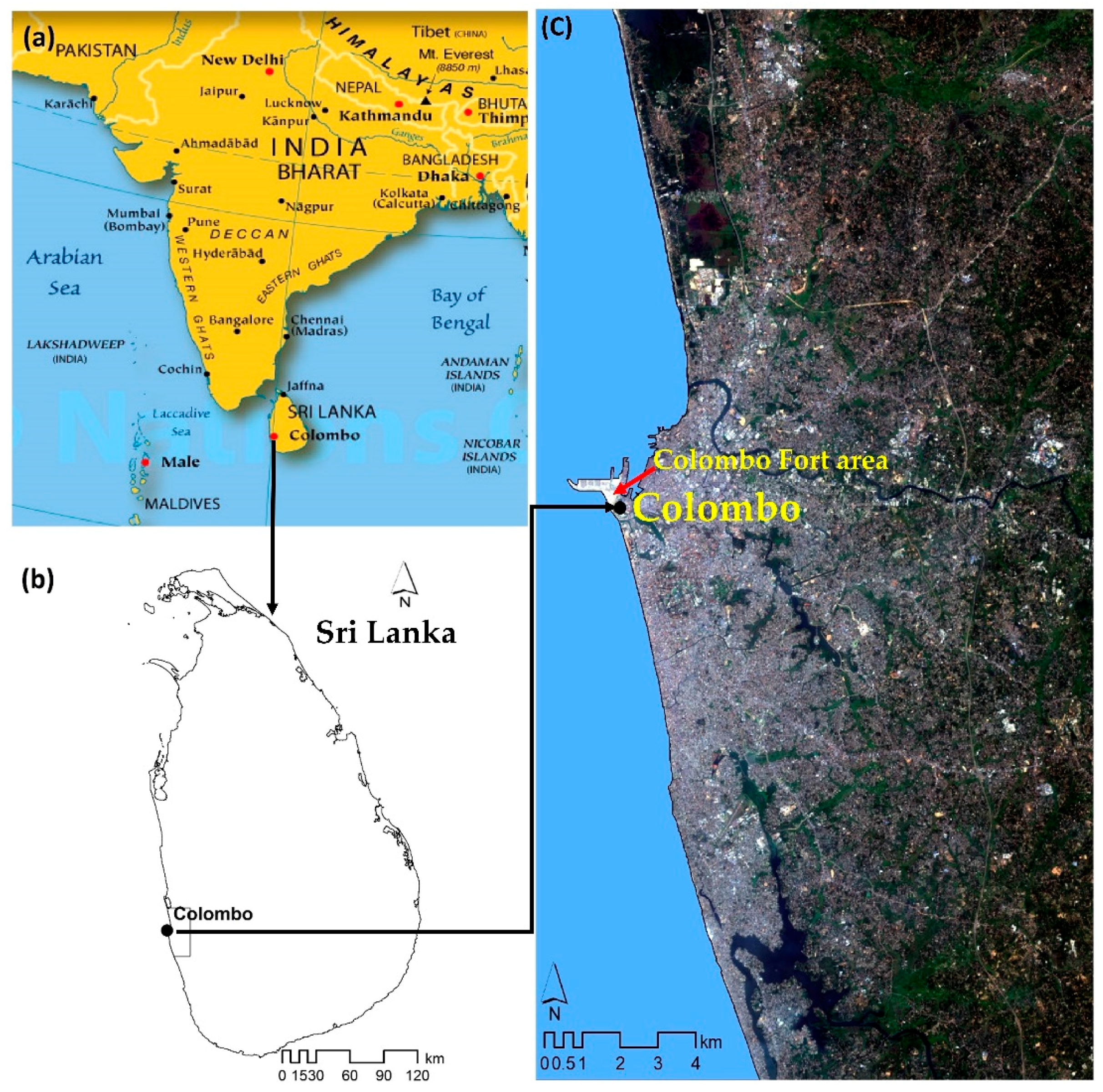
2.1. Study Area: Colombo Metropolitan Area (CMA), Sri Lanka

The CMA is located in the western province of Sri Lanka (Figure 1). It is the country’s most important administrative, industrial and commercial center. To its west is the Indian Ocean.
The CMA is located in a lowland region with a typical hot humid climate. The southwest monsoon blows from late May to the end of September, and the northeast monsoon from the end of November to mid-February. Air temperature and humidity are both high during the year. Wind speeds are low during the inter-monsoon periods (March–April and October–November). The average annual rainfall is 2300 mm. The mean annual temperature is approximately 28 °C [33]. January is the warmest and driest month of the year [31].
The Colombo central business district (CBD) is located near the Colombo Fort area. Its main transportation hubs, such as the main railway station, central bus terminal, and harbor are located in the Colombo Fort area.

2.2. Data Descriptions and Pre-Processing

In this study, we used Landsat images acquired in the dry season, specifically on 7 February 1997, 2 January 2007 (Landsat-5 TM) and 13 January 2017 (Landsat-8 OLI/TIRS) (Table 1). The multispectral bands of the Landsat-5 TM data (bands 1–5 and 7) have 30 m spatial resolution, while the thermal band (band 6) has 120 m spatial resolution, which has been resampled to 30 m by the United States Geological Survey (USGS) (https://landsat.usgs.gov). For the Landsat-8 OLI/TIRS data, the multispectral bands (bands 1–7 and 9) also have 30 m spatial resolution. Its panchromatic band (band 8) has 15 m spatial resolution, while its thermal bands (band 10 and 11) have 100 m spatial resolution, which have also been resampled to 30 m by the USGS (https://landsat.usgs.gov). During the selection of image data, cloud-free images (<10%) were considered.
In this study, we used preprocessed datasets downloaded from http://earthexplorer.usgs.gov. All the images used had undergone standard terrain and atmospheric correction (Level 1T) processing (https://landsat.usgs.gov). They have been geo-referenced to the WGS84/UTM 44 N projection system. The digital number (DN) values of the multispectral bands have been converted into surface reflectance values, while those of the thermal bands have been converted into at-satellite brightness temperature expressed in degrees Kelvin [34,35].

2.3. Land Surface Temperature (LST) Retrieval

The general method to extract LST from raw Landsat datasets requires the conversion of the DN values of the thermal bands into radiance values, which are then used to derive at-satellite brightness temperatures [4,16,36]. Here, we used the preprocessed thermal bands containing at-satellite brightness temperatures expressed in degrees Kelvin. To retrieve the LST values, we first derived the land surface emissivity (ε) values Equation (1) [37].
ε = m PV + n
where m = (ε − ε) − (1 − εσ) Fεv and n = εs + (1 − εs) Fεv, where εs and εv are the soil emissivity and vegetation emissivity, respectively. In this study, we used the result of [37] for m = 0.004 and n = 0.986. PV is the proportion of vegetation extracted from the NDVI Equation (2).
PV = ((NDVI − NDVImin)/(NDVImax − NDVImin))2
where NDVI is the normalized difference vegetation index derived in Equation (4) (see Section 2.4). The NDVImin and NDVImax are the minimum and maximum values of the NDVI, respectively.
The emissivity-corrected LST values were then retrieved using Equation (3).
LST (°C) = TB/1 + (λ × TB/ρ)lnε
where TB = Landsat TM Band 6 at-satellite brightness temperature; λ = wavelength of emitted radiance (λ = 11.5 μm for Landsat TM Band 6, λ = 10.8 μm for Landsat TIRS Band 10) [3]; ρ = h × c/σ (1.438 × 10 – 2 mK), σ = Boltzmann constant (1.38 × 10 − 23 J/K), h = Planck’s constant (6.626 × 10 − 34 Js), c = velocity of light (2.998 × 10⁸ m/s), ε is the land surface emissivity. We later converted the retrieved LST values from degrees Kelvin to degrees Celsius (°C).

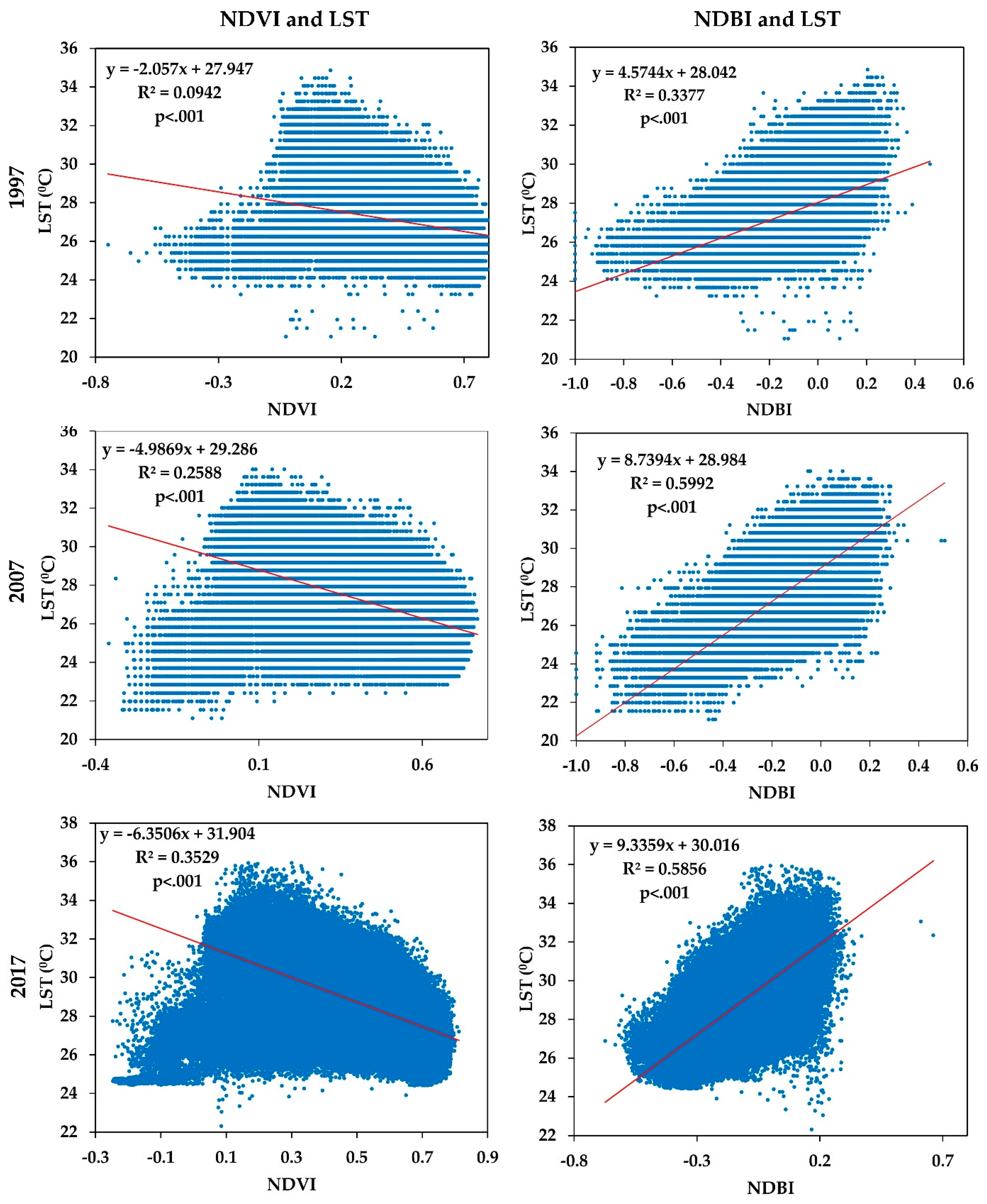
2.4. Normalized Difference Vegetation Index (NDVI) and Normalized Difference Built-Up Index (NDBI)

The NDVI is a major indicator of urban climate [25]. It provides indications of the presence of vegetation and amount or condition of vegetation on pixel basis [38]. The NDVI is derived by using the surface reflectance of the red band (band 3 in TM and band 4 in OLI) and the surface reflectance of the near-infrared band (band 4 in TM and band 5 in OLI) Equation (4) [4,6,39]. The NDVI values range from −1 to 1, with positive values representing vegetated areas and negative values representing non-vegetated areas [25].
NDVI = (NIR − RED)/(NIR + RED)
where NIR = band 4 (for Landsat TM—wavelength 0.76–0.90 µm) and band 5 (for Landsat OLI—wavelength 0.85–0.88 µm) and RED = band 3 (for Landsat TM—wavelength 0.63–0.69 µm) and band 4 (for Landsat OLI—wavelength 0.64–0.67 µm).
The NDBI, on the other hand, is an index for identifying and classifying built-up areas or impervious surfaces [24]. The positive values of the NDBI indicate built-up areas and those close to 0 indicate vegetation, while the negative values represent water bodies [24,39]. The NDBI is expressed as Equation (5):
NDBI = (MIR − NIR)/(MIR + NIR)
where MIR = band 5 (for Landsat TM—wavelength 1.55–1.75 µm) and band 6 (for Landsat 8—wavelength 1.57–1.65 µm) and NIR = band 4 (for Landsat TM—wavelength 0.76–0.90 µm) and band 5 (for Landsat OLI—wavelength 0.85–0.88 µm).

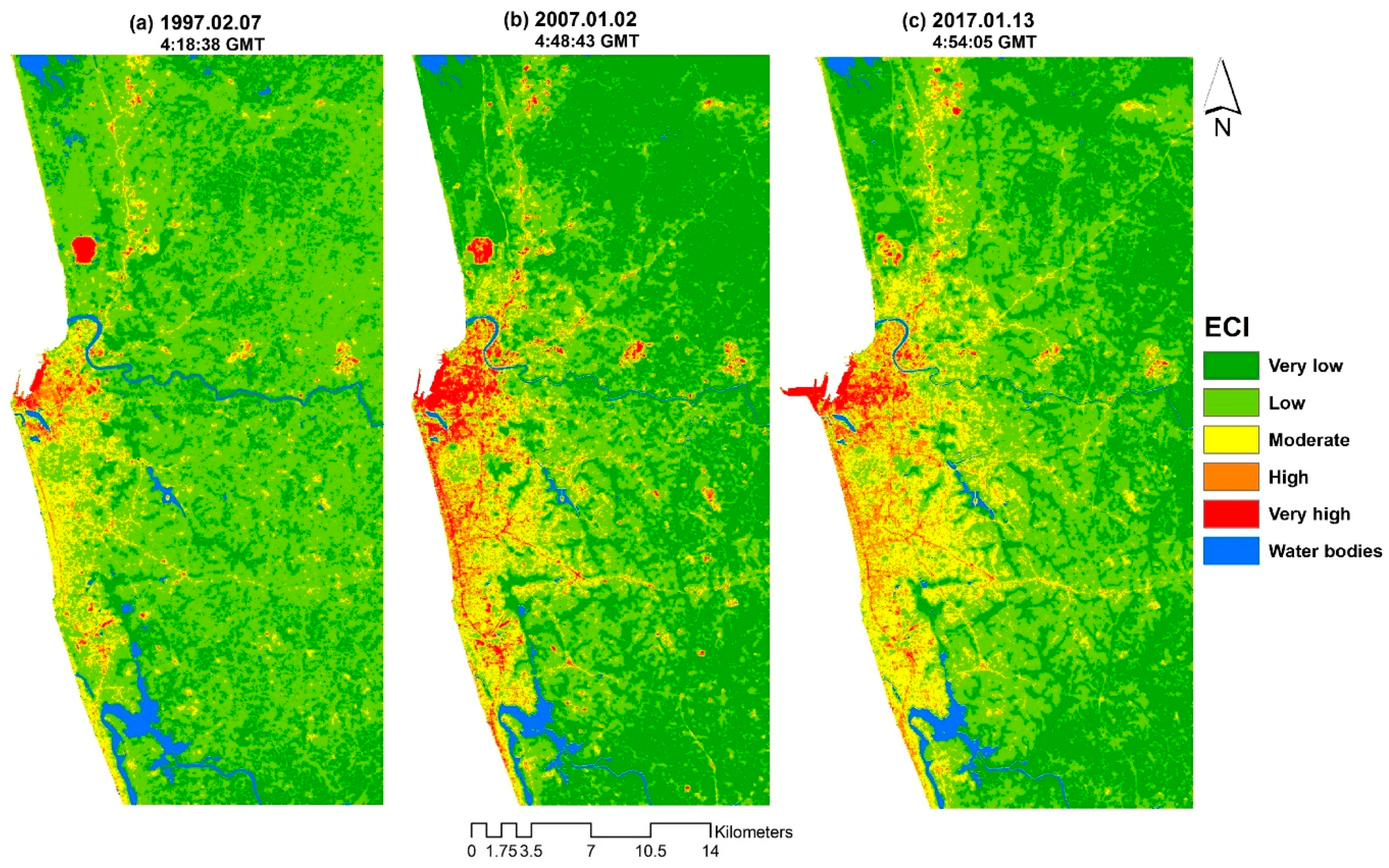
2.5. Environmental Criticality Index (ECI)

The Environmental Criticality Index (ECI) is used to identify environmentally critical areas based on the ratio between LST and NDVI [3]. The LST and NDVI layers used to derive the ECI Equation (6) were first normalized using the histogram equalization method, resulting in a 1–255 pixel value range [3,38]. The higher the ECI value, the more environmentally critical the area is. To facilitate our analysis, we classified the ECI values into five categories, as follows: very low (≤0.5), low (0.5–1), moderate (1–1.5), high (1.5–2.0), and very high (≥2.0).
ECI = LST (Stretched 1–255)/NDVI (Stretched 1–255)
In this analysis, water bodies were excluded. Water bodies were extracted using the modified normalized difference water index (MNDWI) Equation (7) [4,40,41]. Manually calibrated thresholds were used to separate water from non-water areas.
MNDWI = (Green − SWIR1)/(Green + SWIR1)
where Green = band 2 (Landsat TM—wavelength 0.52–0.60 µm) and band 3 (Landsat 8—wavelength 0.53–0.59 µm) and SWIR1 = band 5 (Landsat TM—wavelength 1.55–1.75 µm) and band 6 (Landsat OLI—wavelength 1.57–1.65 µm).

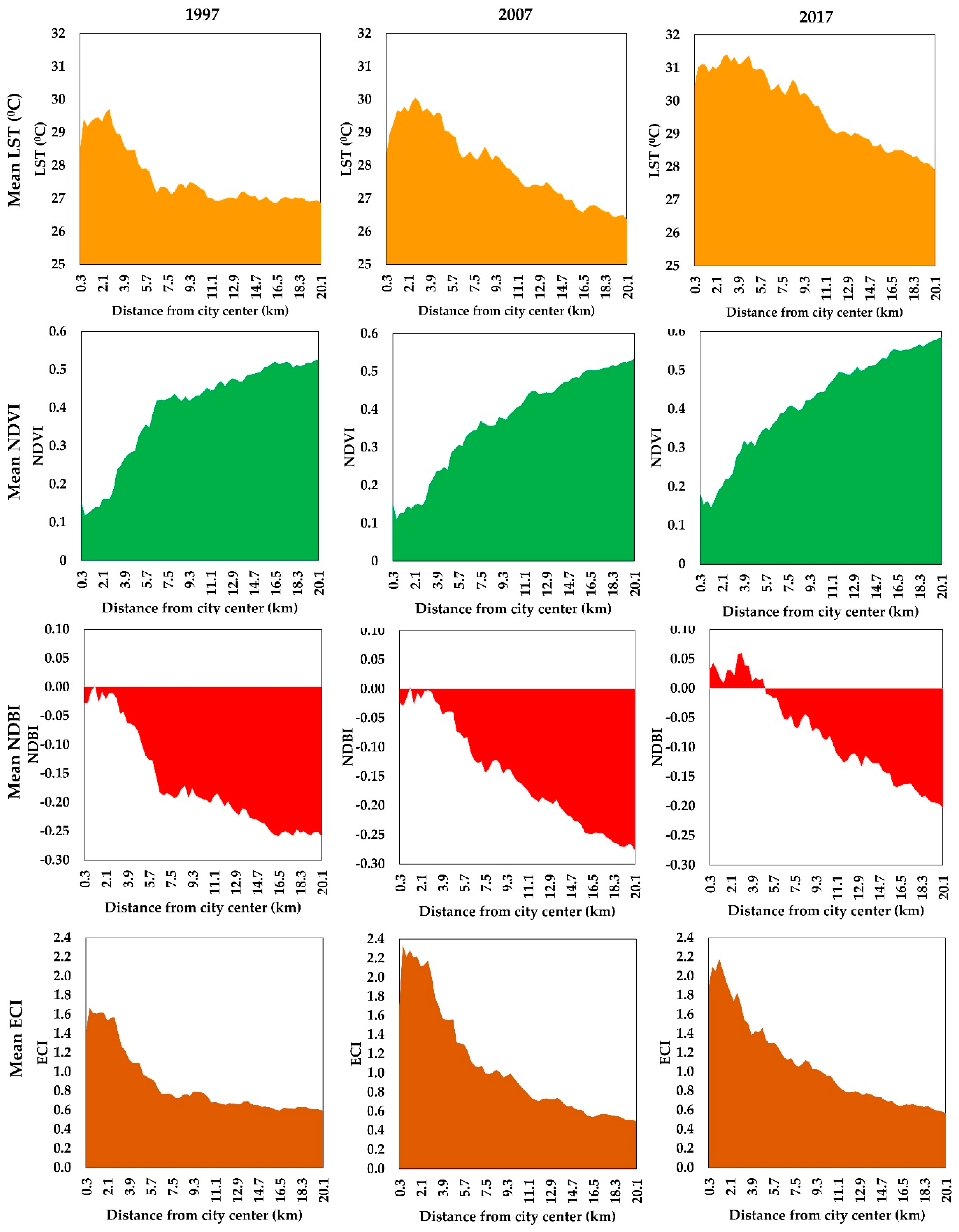
2.6. Urban-Rural Gradient Analysis

This analysis determines the spatial pattern of mean LST, NDVI, NDBI and ECI along the urban–rural gradient of CMA in 1997, 2007 and 2017. Multiple ring buffer zones around the city center (latitude 6°56′4.84″ N, longitude 79°50′34.12″ E) with a distance interval of 300 m were first created. Subsequently, the mean LST, NDVI, NDBI and ECI values were determined in each zone and plotted across the urban–rural gradient. Water bodies were excluded in the analysis.

2.7. Statistical Analysis

Scatter plots were created and a linear regression analysis was performed to determine the relationship between LST and NDVI, and between LST and NDBI. To do this, all the pixels of the study area were first converted into points. The parameter values of these points were then extracted from the LST, NDVI, and NDBI maps. A total of more than 0.869 million pixels were used in this statistical analysis.

3. Results

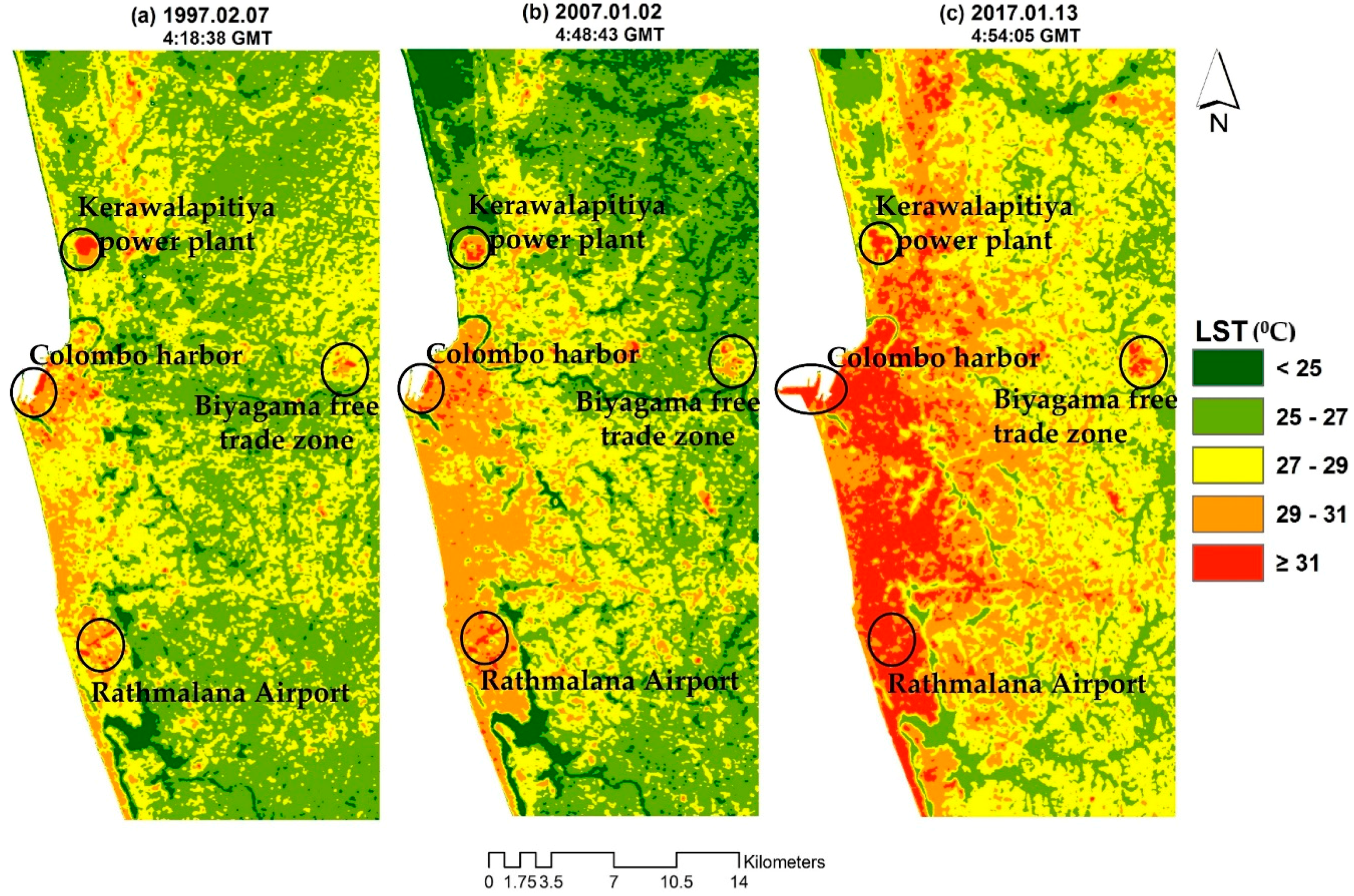
3.1. LST in 1997, 2007 and 2017

The LST maps of CMA in 1997, 2007 and 2017 are shown in Figure 2 and the descriptive statistics of the retrieved LST values are summarized in Table 2. On 7 February 1997 (04:18:38 GMT), the LST in CMA ranged from 21.06–34.86 °C, with a mean of 26.98 °C. On 2 January 2017 (04:48:43 GMT), it varied in the range of 21.10 °C and 34.02 °C, with a mean of 26.96 °C. On 13 January 2017 (04:54:03 GMT), it ranged from 22.31–35.94 °C, with a mean of 28.62 °C. In general, higher LST values were found mostly along the coastal belt, the more urbanized part of the CMA. In 1997 and 2007, areas with high LST were mostly concentrated near the Colombo harbor, Ratmalana Airport, and the Kerawalapitiya power plant area (Figure 2). By 2017, however, areas with high LST had greatly expanded towards the northern, southern and eastern parts of the CMA, following the spatial pattern of urban development in the area. It can also be observed that the LST values of the areas where the free trade zones (e.g., Biyagama free trade zone) and large factories are located have also increased across the three time points (Figure 2).

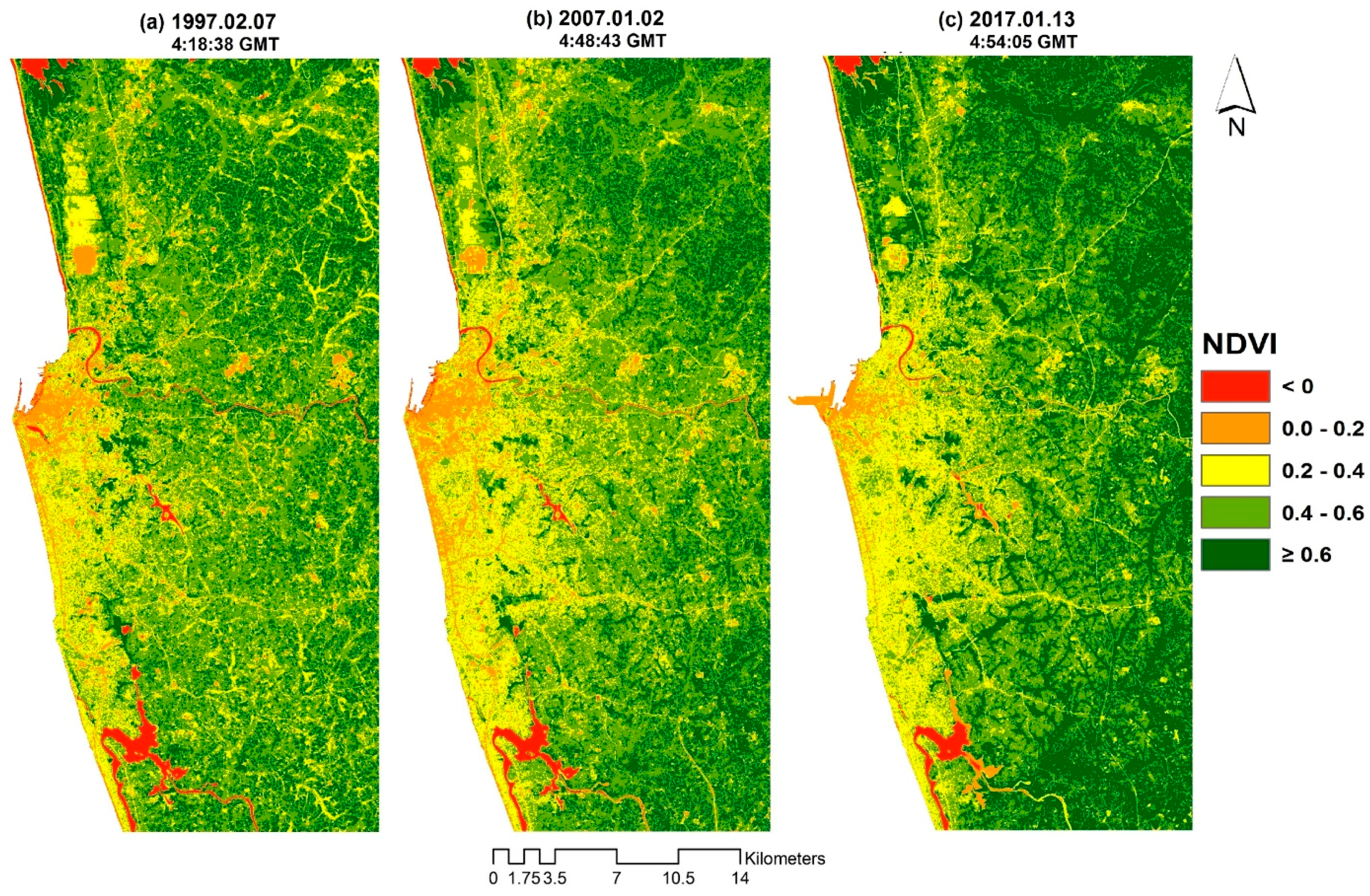
3.2. NDVI in 1997, 2007 and 2017

The NDVI maps of CMA in 1997, 2007 and 2017 are shown in Figure 3 and their descriptive statistics are summarized in Table 3. The NDVI values ranged from −0.74 to 0.84 in 1997, −0.36 to 0.77 in 2007 and −0.25 to 0.81 in 2017. In all three time points, areas with high NDVI values were located mostly in the northeastern, southeastern and eastern parts of the CMA. Wetland areas and cultivated lands both had high NDVI values.
Figure 4 shows the scatterplots between NDVI and LST. The regression analysis revealed that LST is negatively correlated with NDVI across all three time points. Although the coefficient of determination (R2) values were not that high for all three time points, especially in 1997, they were all statistically significant (p < 0.001). In addition, the increasing trend of the R2 values indicates that the explanatory or predictive power of NDVI on the spatial variations of LST became stronger between 1997, 2007 and 2017 as the area became more urbanized.

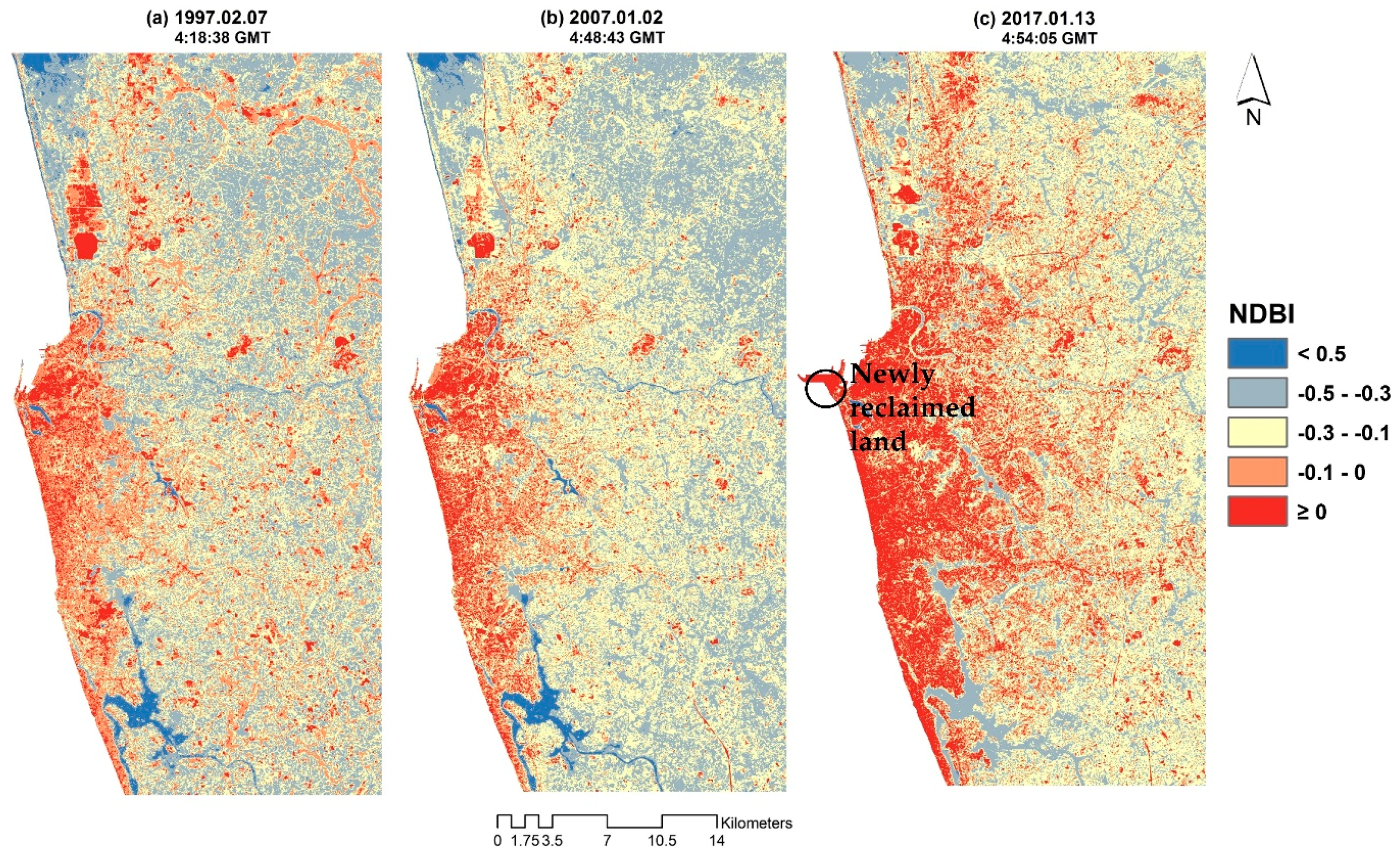
3.3. NDBI in 1997, 2007 and 2017

The NDBI maps of the CMA in 1997, 2007 and 2017 are shown in Figure 5 and their descriptive statistics are summarized in Table 4. The NDBI values ranged from −0.1 to 0.46 in 1997, −0.1 to 0.05 in 2007 and −0.67 to 0.66 in 2017. In 1997 and 2007, areas with high NDBI values were concentrated mostly near the city center and along the coastal belt. But by 2017, areas with high NDBI values had greatly expanded outside the city center, towards the northern, southern, and eastern parts of the CMA. The rapid expansion of areas with high NDBI values from 2007 to 2017 was due to the high rate of urban development during this period, as mentioned earlier (Section 1). The newly reclaimed lands (Figure 5) near the Colombo harbor also had high NDBI values due to the ongoing construction activities in the area, which started in 2014.
It can be observed that the spatial pattern of NDBI values (Figure 5) considerably mirrors the spatial pattern of LST values (Figure 2), indicating a positive linear relationship. The correlation between NDBI and LST was low in 1997, and this could be because the area was still less urbanized. It can be noted that the correlation increased considerably as the area became more urbanized. Nevertheless, like the relationship between NDVI and LST, the relationship between NDBI and LST at the three time points was also statistically significant (p < 0.001), despite the ‘not so high’ correlations. Generally, the relationship between NDBI and LST was stronger than the relationship between NDVI and LST (Figure 4). This indicates that the predictive or explanatory power of NDBI with regards to the spatial pattern of LST in the study area is stronger than that of NDVI.

3.4. ECI in 1997, 2007 and 2017

The ECI maps of the CMA in 1997, 2007 and 2017 are shown in Figure 6. In 1997, 0.6% of the study area had a very high ECI value, 1.5% had a high value, and 7.3% had a moderate value. In 2007, 2.3% had a very high value, 3.7% had a high value, and 10.1% had a moderate value. And in 2017, 1.2% had very high value, 4.0% had a high value, and 14.4% had a moderate value. In general, areas with higher ECI values are found mostly in the urban areas, while areas with lower ECI values are found mainly in the rural areas. The spatial pattern of the ECI values generally follows the spatial patterns of LST values (Figure 2) and NDBI values (Figure 5).

3.5. Urban–Rural Gradient Analysis

Along the urban–rural gradient of the CMA, it can be observed that the mean LST had a much higher increase during the 2007–2017 period than during the 1997–2007 period (Figure 7). This is consistent with the rapid urban development during the 2007–2017 period discussed earlier. The mean NDVI in the middle distances has decreased over the years (e.g., 5.7–9.0 km). However, in 2017, there were also some slight improvements in the mean NDVI, not only in the rural zones (e.g., 9.3–20.1 km), but also in the zones close to the city center (e.g., 0.3–4.8 km). The mean NDBI increased in almost all zones along the urban–rural gradient, but the increase was also much greater during the 2007–2017 period. The mean ECI also increased between 1997 and 2007 from the city center up to the middle distances (0.3–14.1 km). However, in 2017 it decreased in zones close to the city center (0.6–4.8 km). It can be noted that although the mean LST increased in these zones between 2007 and 2017, there was also an increase in the mean NDVI in these same zones. And this is the reason why the mean ECI has decreased in said zones during said period.

4. Discussion

Overall, our results show that the CMA has undergone a process of rapid urbanization in recent decades, but more especially during the 2007–2017 period. Such an urbanization trend has resulted in more intense SUHI effects, as indicated by the increase of areas with higher surface temperature. Here, to better understand these trends, we briefly discuss the historical urban development of the CMA. Afterwards, we will discuss the formation of SUHI and its implications for sustainable landscape and urban planning in the CMA.

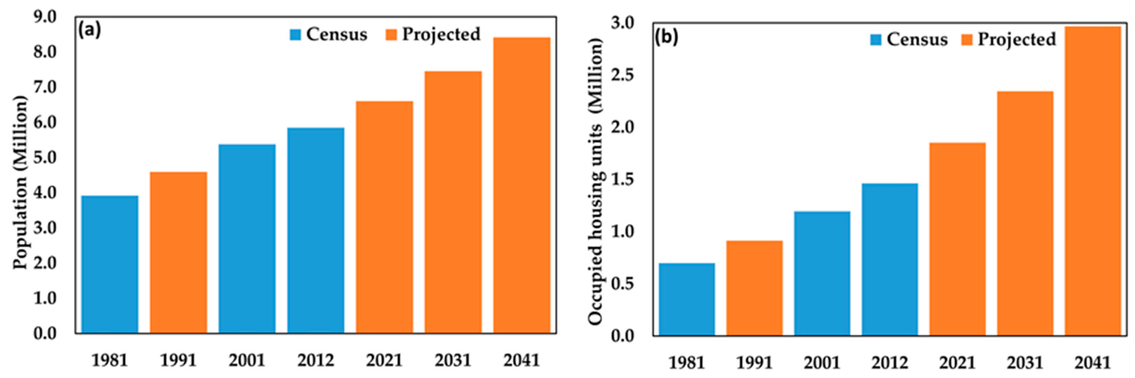
4.1. The Urbanization of the CMA

Colombo City is the main city of the CMA. It is located in the western province of Sri Lanka and serves as the commercial city of the country. Colombo City was ruled by the Portuguese from 1505 to 1656, the Dutch from 1656 to 1796, and the British from 1797 to 1948 [42]. Since the oldest times, Colombo Harbor has been one of the prominent places in South Asia due to its central location in the east–west trade zone of the Indian Ocean. Its popularity among traders, alongside with its strategic location, played an important role in its urban development. Owing to various urban development projects, Colombo City has transformed into a highly urbanized city in the South Asian region [3]. In the past, most of the development activities were concentrated around the port area, presently known as Pettah and Fort. But at the turn of the 21st century, urban development patterns in the area have been influenced by the Colombo Regional Development Strategies under the Colombo Metropolitan Regional Structure Plan (CMRSP)—2000, a plan designed for the development of the Colombo Metropolitan Region (CMR) [42]. As of 2012, approximately 15% of the total urban population of the country lives in Colombo City [43]. According to the Census of Population and Housing 2012, Colombo City has a resident population of 561,314 and a daily floating population of 400,000 [44], making Colombo the densest city in the island (15,170 people per km2) [43]. The ‘daily floating population’ includes people who come to the city, but are not officially registered as residents.
Figure 8a shows that the population of the western province of Sri Lanka where the CMA is located has been continuously increasing. According to the census data in 2012, the CMA accounts for 62% of the population of the province [45]. Similarly, occupied housing units have also been continuously increasing in the western province of Sri Lanka (Figure 8b). Accordingly, the CMA accounts for 60% of the total occupied housing units of the province [45]. These increasing trends of population and housing are expected to continue in the future (Figure 8). However, the challenge will be on the availability of land for housing, as well as appropriate zoning plans, in order to facilitate these predicted urban growth developments. It is important to consider the provisions of more green spaces, because green spaces can help mitigate urban warming effects.
Compared with the other South Asian countries, Sri Lanka has recorded one of the highest gross domestic product (GDP) rates per capita from 2008 (Figure 9). It reached up to US$3926 in 2015. In the past, the growth of Sri Lanka’s economy was heavily affected by various factors, including the Janatha Vimukthi Peramuna (JVP) revolution (1987–1989) and civil war in (1983–2009) [29]. However, after the conclusion of the civil war in 2009, more urban development projects have been carried out in Sri Lanka and most of them are located in the CMA [3]. These recent developments are major factors in the rapid growth of the country’s GDP in recent years (Figure 9).
Indeed, the results show that CMA’s urbanization was more rapid during the 2007–2017 period compared with 1997–2007 (Figure 2 and Figure 5). This rapid urbanization is expected to continue in the future, as also predicted by Subasinghe et al. [29]. Being the only metropolitan area in the country, the CMA has strong economic growth. Most of the country’s commercial centers, administrative centers, and headquarters are located in the CMA [29]. In 2014, a new port city development project was started near the Colombo harbor [29]. This urban development initiative is expected to contribute to the expansion of urban areas to the west side of Colombo City. It is also expected that this project will increase the daily floating population in the near future. The CMA has a prominent location in the Indian Ocean (new Silk Road economic belt) [48], which is important for foreign direct investments. At present, more than 80% of industries are located in the CMA [29,32].
In general, the urbanization pattern of the CMA has two significant spatial features: (1) in the past, more urban areas were concentrated near the city center and harbor and have had a linear distribution along the road network and along the coastal belt [42]; and (2) at present, urban areas have been rapidly expanding to the northern, southern and eastern parts of the CMA. As mentioned earlier, rapid infrastructural development had occurred during the past decade (2007–2017) after the conclusion of the civil war in May 2009, which resulted in various road construction and development projects, as well as urban beautification projects, which also contributed to the urbanization pattern in the CMA [3]. Consequently, however, this urbanization has replaced a considerable portion of the natural land surface of the CMA with impervious surfaces. And as our results show, these landscape changes have contributed to the formation of SUHI in CMA (Figure 2 and Figure 5) (more on this below).

4.2. The Formation of SUHI and Its Implications for Sustainable Landscape and Urban Planning in the CMA

The rapid expansion of built-up lands and intensifying SUHI effects that we observed in this study (Figure 2 and Figure 5) are consistent with the recent developments discussed above. Due to urban development, more open and vegetated areas have been replaced with impervious surfaces such as building, roads, parking lots, pavements and other constructions [3]. We recognize that the detected temporal variation in the overall mean LST might have been influenced by the given environmental conditions at the time when the satellite images were captured. However, we are also inclined to hypothesize that the observed increase in the overall average LST in the CMA from 1997–2017 (i.e., 1.64 °C) might have been mainly due to the rapid urbanization of the area. The significant correlations between LST and both NDVI (negative) and NDBI (positive) (Figure 4) that we found in this study support this proposition and are also consistent with other previous findings [10,25]. The low correlation (negative) between NDVI and LST that we observed in this study (Figure 4) was due to the inclusion of wetland areas and water bodies in the statistical analysis. These areas had low NDVI and LST values. The points representing these areas are reflected in the lower left section of the scatter plots that show the relationship between NDVI and LST (Figure 4). Other similar studies have also shown that, indeed, NDVI can have a low negative correlation with LST [20,25].
While indications of increasing LST in the CMA (Figure 2 and Figure 7) appear parallel to the expansion of impervious surfaces (Figure 5 and Figure 7), there have also been indications of both vegetation loss (1997–2007) and improvement (2007–2017) (Figure 3 and Figure 7). In the context of the UHI phenomenon, although current efforts focus on the effects of urban design and geometry on wind flow, including the size, shape and orientation of buildings, and other possible mitigation and adaptation measures including the use of green roofs, cool roofs and cool pavements, the abundance and spatial pattern of green spaces in urban areas are still important [2,4]. In the CMA, we recognize the efforts of the local government for initiating urban development programs that could also improve the status of urban green spaces in the area [3,29]. In fact, our results show that in the CMA, the area of land with ‘very high’ ECI values has decreased (2007–2017) despite the increase in LST, and this has been due to the increase in the NDVI values (Figure 6, Section 3.4).
That being said, the area of lands with ‘high’ and ‘moderate’ ECI values have been continuously increasing (1997–2017) and expanding outward of the city center (Figure 6 and Figure 7). Thus, we recommend that such efforts on urban greening be continued in order to disrupt this trend and mitigate the warming effects of SUHI in the CMA. The current ECI map of the CMA (2017) produced in this study (Figure 6) can provide some insights of the locations or areas that need some priority. Examples of these areas include the central business district, the areas near the harbor, the coastal belt, the Colombo–Galle (A2) road, the Colombo–Kandy roads (A1), the Colombo–Negombo road (A3), and the High–level road (A4). The transportation network of the CMA plays an important role in the urban development of the area, but also contributes to the loss of green spaces and elevates surface temperature. These findings on the spatial pattern of environmentally critical areas along the transport network are also consistent with some previous findings [3]. Thus, greening activities such as tree planting along the roads are encouraged.

4.3. Limitations of the Study and Future Research

In this study, the satellite images used were not captured in the same time or day of the year. Therefore, the results should be interpreted in the context of this limitation. We also used only two landscape variables (NDVI and NDBI) in examining the spatial and temporal variations of LST. Other variables, including socio-economic variables, also need to be explored and examined in future studies. In addition, the intensity of SUHI (including its spatial and temporal changes), which has not been determined in this study, also needs to be considered in future studies.

5. Conclusions

In this study, we examined the spatiotemporal patterns of LST in the CMA in the context of the SUHI phenomenon using Landsat data (1997–2017). We found indications of intensifying SUHI effects, especially during the 2007–2017 period when urbanization was more rapid. The significant, strong positive correlations between LST and NDBI across all three time points (1997, 2007, and 2017) (p < 0.001) confirm the strong influence of urbanization on the formation of SUHI in the CMA. While there have been indications of vegetation loss, especially from 1997 to 2007, we also found indications of vegetation improvement in some parts of the CMA, especially from 2007 to 2017. We recommend that such efforts on urban greening be continued because urban green spaces can help mitigate warming effects due to SUHI. The ECI map produced in this study can be useful in such undertakings. Needless to say, urban green spaces are also important components of the urban sustainability concept.

Acknowledgments

The corresponding author expresses his gratefulness to the University Grant Commission, Sri Lanka & JASSO Monbukagakusho Honors Scholarship for providing the research grant for carrying out PhD research. This study was partly supported by the Japan Society for the Promotion of Science (JSPS) under a grant for Challenging Exploratory Research (ID No. 16K12816). The comments and suggestions of the anonymous reviewers are gratefully acknowledged.

Author Contributions

The corresponding author, Manjula Ranagalage, proposed the topic and spearheaded the data processing and analysis, as well as the writing of the manuscript. Ronald C. Estoque and Yuji Murayama helped in the design, research implementation and analysis, and writing of the manuscript.

Conflicts of Interest

The authors declare no conflicts of interest.

References

  1. United Nations. World Urbanization Prospects: The 2014 Revision: Highlights; United Nations: New York, NY, USA, 2015. [Google Scholar]
  2. Estoque, R.C.; Murayama, Y. Measuring sustainability based upon various perspectives: A case study of a hill station in Southeast Asia. Ambio 2014, 43, 943–956. [Google Scholar] [CrossRef] [PubMed]
  3. Senanayake, I.P.; Welivitiya, W.D. D.P.; Nadeeka, P.M. Remote sensing based analysis of urban heat islands with vegetation cover in Colombo city, Sri Lanka using Landsat-7 ETM+ data. Urban Clim. 2013, 5, 19–35. [Google Scholar] [CrossRef]
  4. Estoque, R.C.; Murayama, Y.; Myint, S.W. Effects of landscape composition and pattern on land surface temperature: An urban heat island study in the megacities of Southeast Asia. Sci. Total Environ. 2017, 577, 349–359. [Google Scholar] [CrossRef] [PubMed]
  5. Howard, L. The Climate of London; W. Phillips: London, UK, 1818. [Google Scholar]
  6. Kikon, N.; Singh, P.; Singh, S.K.; Vyas, A. Assessment of urban heat islands (UHI) of Noida City, India using multi-temporal satellite data. Sustain. Cities Soc. 2016, 22, 19–28. [Google Scholar] [CrossRef]
  7. EPA (US Environmental Protection Agency). Reducing Urban Heat Islands: Compendium of Strategies Urban Heat Island Basics; US Environmental Protection Agency: Washington, DC, USA, 2009.
  8. Rizwan, A.M.; Dennis, L.Y.C.; Liu, C. A review on the generation, determination and mitigation of Urban Heat Island. J. Environ. Sci. 2008, 20, 120–128. [Google Scholar] [CrossRef]
  9. Rogan, J.; Ziemer, M.; Martin, D.; Ratick, S.; Cuba, N.; DeLauer, V. The impact of tree cover loss on land surface temperature: A case study of central Massachusetts using Landsat Thematic Mapper thermal data. Appl. Geogr. 2013, 45, 49–57. [Google Scholar] [CrossRef]
  10. Kumar, D.; Shekhar, S. Statistical analysis of land surface temperature-vegetation indexes relationship through thermal remote sensing. Ecotoxicol. Environ. Saf. 2015, 121, 39–44. [Google Scholar] [CrossRef] [PubMed]
  11. Dousset, B.; Gourmelon, F. Satellite multi-sensor data analysis of urban surface temperatures and landcover. ISPRS J. Photogramm. Remote Sens. 2003, 58, 43–54. [Google Scholar] [CrossRef]
  12. Aniello, C.; Morgan, K.; Busbey, A.; Newland, L. Mapping micro-urban heat islands using LANDSAT TM and a GIS. Comput. Geosci. 1995, 21, 965–969. [Google Scholar] [CrossRef]
  13. Stathopoulou, M.; Cartalis, C. Daytime urban heat islands from Landsat ETM+ and Corine land cover data: An application to major cities in Greece. Sol. Energy 2007, 81, 358–368. [Google Scholar] [CrossRef]
  14. Weng, Q.; Lu, D.; Schubring, J. Estimation of land surface temperature-vegetation abundance relationship for urban heat island studies. Remote Sens. Environ. 2004, 89, 467–483. [Google Scholar] [CrossRef]
  15. Chen, X.L.; Zhao, H.M.; Li, P.X.; Yin, Z.Y. Remote sensing image-based analysis of the relationship between urban heat island and land use/cover changes. Remote Sens. Environ. 2006, 104, 133–146. [Google Scholar] [CrossRef]
  16. Weng, Q. Thermal infrared remote sensing for urban climate and environmental studies: Methods, applications, and trends. ISPRS J. Photogramm. Remote Sens. 2009, 64, 335–344. [Google Scholar] [CrossRef]
  17. Li, J.; Song, C.; Cao, L.; Zhu, F.; Meng, X.; Wu, J. Impacts of landscape structure on surface urban heat islands: A case study of Shanghai, China. Remote Sens. Environ. 2011, 115, 3249–3263. [Google Scholar] [CrossRef]
  18. Li, Y.Y.; Zhang, H.; Kainz, W. Monitoring patterns of urban heat islands of the fast-growing Shanghai metropolis, China: Using time-series of Landsat TM/ETM+ data. Int. J. Appl. Earth Obs. Geoinf. 2012, 19, 127–138. [Google Scholar] [CrossRef]
  19. Bokaie, M.; Zarkesh, M.K.; Arasteh, P.D.; Hosseini, A. Assessment of urban heat island based on the relationship between land surface temperature and land use/land cover in Tehran. Sustain. Cities Soc. 2016, 23, 94–104. [Google Scholar] [CrossRef]
  20. Zhang, X.; Estoque, R.C.; Murayama, Y. An urban heat island study in Nanchang City, China based on land surface temperature and social-ecological variables. Sustain. Cities Soc. 2017, 32, 557–568. [Google Scholar] [CrossRef]
  21. Alves, E. Seasonal and spatial variation of surface urban heat island intensity in a small urban agglomerate in Brazil. Climate 2016, 4, 61. [Google Scholar] [CrossRef]
  22. Tran, H.; Uchihama, D.; Ochi, S.; Yasuoka, Y. Assessment with satellite data of the urban heat island effects in Asian mega cities. Int. J. Appl. Earth Obs. Geoinf. 2006, 8, 34–48. [Google Scholar] [CrossRef]
  23. Liu, L.; Zhang, Y. Urban heat island analysis using the landsat TM data and ASTER Data: A case study in Hong Kong. Remote Sens. 2011, 3, 1535–1552. [Google Scholar] [CrossRef]
  24. Zha, Y.; Gao, J.; Ni, S. Use of normalized difference built-up index in automatically mapping urban areas from TM imagery. Int. J. Remote Sens. 2003, 24, 583–594. [Google Scholar] [CrossRef]
  25. Zhang, Y.; Odeh, I.O.A.; Han, C. Bi-temporal characterization of land surface temperature in relation to impervious surface area, NDVI and NDBI, using a sub-pixel image analysis. Int. J. Appl. Earth Obs. Geoinf. 2009, 11, 256–264. [Google Scholar] [CrossRef]
  26. Yuan, F.; Bauer, M.E. Comparison of impervious surface area and normalized difference vegetation index as indicators of surface urban heat island effects in Landsat imagery. Remote Sens. Environ. 2007, 106, 375–386. [Google Scholar] [CrossRef]
  27. Li, J.; Wang, X.; Wang, X.; Ma, W.; Zhang, H. Remote sensing evaluation of urban heat island and its spatial pattern of the Shanghai metropolitan area, China. Ecol. Complex. 2009, 6, 413–420. [Google Scholar] [CrossRef]
  28. Xiao, R.; Ouyang, Z.; Zheng, H.; Li, W.; Schienke, E.W.; Wang, X. Spatial pattern of impervious surfaces and their impacts on land surface temperature in Beijing, China. J. Environ. Sci. (China) 2007, 19, 250–256. [Google Scholar] [CrossRef]
  29. Subasinghe, S.; Estoque, R.C.; Murayama, Y. Spatiotemporal analysis of urban growth using GIS and remote sensing: A case study of the Colombo Metropolitan Area, Sri Lanka. Int. J. Geo-Inf. 2016, 5, 197. [Google Scholar] [CrossRef]
  30. Emmanuel, R.; Fernando, H.J.S. Urban heat islands in humid and arid climates: Role of urban form and thermal properties in Colombo, Sri Lanka and Phoenix, USA. Clim. Res. 2007, 34, 241–251. [Google Scholar] [CrossRef]
  31. Emmanuel, R.; Johansson, E. Influence of urban morphology and sea breeze on hot humid microclimate: The case of Colombo, Sri Lanka. Clim. Res. 2006, 30, 189–200. [Google Scholar] [CrossRef]
  32. Emmanuel, R. Thermal comfort implications of urbanization in a warm-humid city: The Colombo Metropolitan Region (CMR), Sri Lanka. Build. Environ. 2005, 40, 1591–1601. [Google Scholar] [CrossRef]
  33. Herath, D.; Pitawala, A.; Gunatilake, J. Heavy metals in road deposited sediments and road dusts of Colombo Capital, Sri Lanka. J. Nat. Sci. Found. Sri Lanka 2016, 44, 193–202. [Google Scholar] [CrossRef]
  34. Landsat, T.; User, S.D.; Project, L.; Office, S.; Space, G.; Landsat, U. Landsat 7 Science Data Users Handbook. Available online: https://landsat.gsfc.nasa.gov/wp-content/uploads/2016/08/Landsat7_Handbook.pdf (accessed on 20 June 2017).
  35. USGS Landsat 8 (L8) Data Users Handbook. Version 1.0; June 2015. Available online: https://landsat.usgs.gov/sites/default/files/documents/Landsat8DataUsersHandbook.pdf (accessed on 20 June 2017).
  36. Chander, G.; Markham, B.L.; Helder, D.L. Summary of current radiometric calibration coefficients for Landsat MSS, TM, ETM+, and EO-1 ALI sensors. Remote Sens. Environ. 2009, 113, 893–903. [Google Scholar] [CrossRef]
  37. Sobrino, J.A.; Jiménez-Muñoz, J.C.; Paolini, L. Land surface temperature retrieval from Landsat TM 5. Remote Sens. Environ. 2004, 90, 434–440. [Google Scholar] [CrossRef]
  38. Orhan, O.; Ekercin, S.; Dadaser-Celik, F. Use of Landsat land surface temperature and vegetation indices for monitoring drought in the Salt Lake Basin Area, Turkey. Sci. World J. 2014, 2014, 1–11. [Google Scholar] [CrossRef] [PubMed]
  39. Liu, H.; Weng, Q. Enhancing temporal resolution of satellite imagery for public health studies: A case study of West Nile Virus outbreak in Los Angeles in 2007. Remote Sens. Environ. 2012, 117, 57–71. [Google Scholar] [CrossRef]
  40. Li, W.; Du, Z.; Ling, F.; Zhou, D.; Wang, H.; Gui, Y.; Sun, B.; Zhang, X. A comparison of land surface water mapping using the normalized difference water index from TM, ETM+ and ALI. Remote Sens. 2013, 5, 5530–5549. [Google Scholar] [CrossRef]
  41. Xu, H. Modification of normalised difference water index (NDWI) to enhance open water features in remotely sensed imagery. Int. J. Remote Sens. 2006, 27, 3025–3033. [Google Scholar] [CrossRef]
  42. Sevanatha and Colombo Municipal Council (CMC). Poverty Profile City of Colombo: Urban Poverty Reduction Through Community Empowerment, Colombo. Available online: http://www.ucl.ac.uk/dpu-projects/drivers_urb_change/urb_society/pdf_liveli_vulnera/Sevanatha_Poverty_Profile1.pdf (accessed on 20 June 2017).
  43. Department of Census and Statistics. Census of Population and Housing 2012; Department of Census and Statistics: Colombo, Sri Lanka, 2012.
  44. City of Colombo. Available online: http://colombo.mc.gov.lk/colombo.php (accessed on 15 February 2017).
  45. Census of Population and Housing 2012. Available online: http://www.statistics.gov.lk/pophousat/cph2011/index.php?fileName=Activities/TentativelistofPublications (accessed on 27 May 2017).
  46. The World Bank, World Development Indicators: GDP (Current US$). Available online: http://data.worldbank.org/indicator/NY.GDP.MKTP.CD?locations=LK (accessed on 17 April 2017).
  47. The World Bank. Colombo: The Heartbeat of Sri Lanka. 2013. Available online: http://www.worldbank.org/en/news/feature/2013/03/21/colombo-heartbeat-sri-lanka (accessed on 17 April 2017).
  48. Zimmerman, T. The New Silk Roads: China, the U.S., and the Future of Central Asia. 2015. Available online: http://cic.nyu.edu/sites/default/files/zimmerman_new_silk_road_final_2.pdf (accessed on 27 May 2017).
Figure 1. Location map of the study area: (a) map of South Asia (Map source: www.nationasonline.org); (b) location of Colombo City; (c) the extent of the study area within the Colombo Metropolitan Area (CMA) (Landsat-8 OLI/TIRS in true color composite bands 4, 3, 2).
Ijgi 06 00189 g001
Figure 2. Land surface temperature (LST) maps of the CMA in (a) 1997; (b) 2007; and (c) 2017.
Ijgi 06 00189 g002
Figure 3. Normalized difference vegetation index (NDVI) maps of the CMA in (a) 1997; (b) 2007; and (c) 2017.
Ijgi 06 00189 g003
Figure 4. Scatter plots between NDVI, NDB and LST in 1997, 2007, and 2017.
Ijgi 06 00189 g004
Figure 5. Normalized difference built-up index (NDBI) maps of the CMA in (a) 1997; (b) 2007; and (c) 2017.
Ijgi 06 00189 g005
Figure 6. Environmental Criticality Index (ECI) maps of the CMA in (a) 1997, (b) 2007, and (c) 2017.
Ijgi 06 00189 g006
Figure 7. Patterns of LST, NDVI, NDBI and ECI along the urban–rural gradient of the CMA in 1997, 2007 and 2017.
Ijgi 06 00189 g007
Figure 8. (a) Population growth of the western province. Note: The 1991 population was projected using a 1.6% growth rate (1981–2001). The 2021, 2031 and 2041 populations were projected using a 1.2% growth rate (average between 1981–2001 and 2001–2012); (b) Occupied housing units of the western province. The 1991 data was projected using a 2.7% increase rate (1981–2001). The 2021, 2031 and 2041 data were projected using a 2.4% increase rate (average between 1981–2001 and 2001–2012). (Data Source: Census Data Statistics 1981, 2001, and 2012).
Ijgi 06 00189 g008
Figure 9. GDP of Sri Lanka and other South Asian countries (1990–2015) [46]. Note: Due to the lack of multi-temporal GDP data for the CMA, countrywide data were used as a proxy indicator. The CMA accounts for about 50% of Sri Lanka’s GDP [47].
Ijgi 06 00189 g009
Table 1. Descriptions of the Landsat images used.
SensorScene IDAcquisition DateTime (GMT)Season
Landsat-5 TMLT51410551997038BKT017 February 199704:18:38Dry
Landsat-5 TMLT51410552007002BKT002 January 200704:48:43Dry
Landsat-8 OLI/TIRSLC81410552017013LGN0013 January 201704:54:05Dry
Table 2. Descriptive statistics of the retrieved LST values in CMA (°C).
DateTime (GMT)MinimumMaximumMeanStandard Deviation
7 February 199704:18:3821.0634.8626.981.12
2 January 200704:48:4321.1034.0226.961.57
13 January 201704:54:0522.3135.9428.621.71
Table 3. Descriptive statistics of the NDVI values in the CMA.
DateMinimum Maximum Mean Standard Deviation
7 February 1997−0.750.840.470.17
2 January 2007−0.360.770.470.16
13 January 2017−0.250.810.520.16
Table 4. Descriptive statistics of the normalized difference built-up index (NDBI) values in the CMA.
DateMinimumMaximumMeanStandard Deviation
7 February 1997−1.000.46−0.230.14
2 January 2007−1.000.51−0.230.14
13 January 2017−0.670.66−0.150.14

