Causal Transmission in Reduced-Form Models ^†

Abstract

We propose a method to explore the causal transmission of an intervention through two endogenous variables of interest. We refer to the intervention as a catalyst variable. The method is based on the reduced-form system formed from the conditional distribution of the two endogenous variables given the catalyst. The method combines elements from instrumental variable analysis and Cholesky decomposition of structural vector autoregressions. We give conditions for uniqueness of the causal transmission.

1. Introduction

In general, it is difficult to deduce the causal ordering of two observed variables from their joint distribution. However, if we can assume that a third variable is causal, it may be possible to deduce how the effect of this third variable will transmit between the two variables of interest. By conditioning on a catalyst, the joint distribution of a bivariate system can be used to infer a causal transmission. Our approach allows for different catalysts transmitting through the same two variables in different ways. We formulate this for a general distributional setup.

Philosophers and scientists argue that some background of causal knowledge is required in order to construct new causal facts. The view “no causes in, no causes out” (Cartwright 1989) expresses the concern that we cannot jump from theory to cause without some causal facts in hand. Pearl (2000) similarly underlines the importance of distinguishing between causal and associational concepts, as every causal conclusion relies on a causal assumption that is untested in observational studies. In contrast, Granger (1969) causality is an example of an associational concept seeking to infer correlations from data without a causal assumption. Moreover, Granger causality is concerned with temporal correlations as opposed to the ordering of contemporaneous variables. Causal analysis goes one step further by inferring correlations under changing conditions.

We combine elements from instrumental variable analysis and recursive ordering of structural vector autoregressions. Instrumental variable analysis will in general not order the endogenous variables but can be used to identify a structural relation uniquely. Cholesky decomposition orders endogenous variables, but the ordering is not unique. By carrying out a Cholesky decomposition in the presence of an instrument, there is scope for a unique ordering which is interpretable as a causal transmission. In this situation we will refer to the instrument as a catalyst.

The catalyst w may transmit causally through the variables $y,z$. It is possible that w transmits through z to y or through y to z or, of course, that there is no ordering of the variables. We present two sets of testable conditions. A first set of conditions is needed for establishing that the catalyst w transmits through z to y, say, in a unique fashion. A second set of conditions is needed for showing that w actually affects y. The econometric framework is a reduced form based on the conditional distribution of $y,z$ given w. The theory is formulated for general densities but with special attention to the most common cases, which include the bivariate normal distribution and mixtures of a univariate normal distribution with a logit or probit distribution.

We can identify catalysts from the analysis of past events, exploiting interventions that were determined separately from the realization of endogenous variables. Careful judgement of the situation at hand will be needed. For instance, in the context of our empirical illustration of the UK demand for narrow money, we will consider reduction in the value added tax (VAT) to be an intervention. While the VAT reduction will be a reaction to the state of the UK economy, the objective was specifically to boost demand rather than to impact money demand (Cloyne 2013). Our interpretation is that there may be some important causal transmission channels at work, which we can learn about through econometric analysis. If we are able to find a causal transmission, then we can hope that a future intervention of the same type may transmit in the same manner. We restrict the analysis to the bivariate setup in order to be as clear as possible. Larger systems can have many possible transmission channels, which will be examined in future work.

Causal transmission is similar to but distinct from super exogeneity (Engle et al. 1983). Hendry (1995, pp. 176–77) argues that causation between two variables of interest—money and inflation—could be investigated through super exogeneity. One of the conditions is that the conditional distribution of one variable $y_t$ given $z_t$ is invariant under interventions to $z_t$. In contrast, our notion of causal transmission is concerned with the propagation of specific shocks to the system of the variables $y_t$, $z_t$. It allows the possibility that different shocks can flow through a system of variables in different directions. The empirical illustration provides an example of this property. Our analysis is inspired by the invariance to interventions but with a focus on the transmission of the shock through y, z rather than on the conditional relation of y given z.

Our notion of causal transmission also bears many similarities to the graphical modeling literature, see, for instance Dawid (1979), Lauritzen (1996), Pearl (2000), and Cox and Wermuth (2004). We operate exclusively in the conditional distribution of $y,z$ given w, leaving w unmodeled, as our aim is to discover how the w transmits through $y,z$. Causal search over graphical models is usually formulated in the unconditional distribution of $y,z,w$ (Spirtes et al. 2000), while our particular setup takes the asymmetry of w as given and could be referred to as a chain graph with components $\left\{w\right\}$ and $\{y,z\}$ (Drton 2009). The idea of exploring conditional structures can be found in Lauritzen and Wermuth (1989), Andersson et al. (2001), and Cox and Wermuth (2003). To describe the transmission, we will look for both conditional independences and conditional dependences. The latter have been addressed by, for instance, Wermuth and Sadeghi (2012). The graphical modeling literature often works through correlations and therefore requires normality, while we work with general distributions. For this, we have found inspiration in Lauritzen (1996).

In Section 2, we provide a motivating example for the case of a bivariate normal setup. In Section 3, we define and explore causal transmissions. In Section 4, we generalize the idea to situations with multiple catalysts which transmit through the variables of interest in different ways and we offer a structural interpretation that combines Cholesky decomposition and instrumental variable estimation. Section 5 compares our use of graphs to describe transmission of multiple catalysts with the use of graphs in the graphical model literature, and it gives an overview of the associated exponential family properties. An empirical illustration using a UK monetary data set follows in Section 6. Section 7 concludes. Proofs are given in Appendix A.

2. Introductory Example

We think of causal transmission as being asymmetric by nature: influence flows one way and cannot be reversed. Here, we introduce the ideas in a bivariate normal setup.

Suppose we are interested in an economic relationship between two endogenous, or modeled, variables $(y,z)$ given a third variable w. Thus, we are interested in the conditional distribution $\mathsf{f}(y,z|w)$. Under normality, the distribution of $y,z$ given w is given by

$$\begin{array}{c}\hfill \left(\begin{array}{c}y\\ z\end{array}\right)=\left(\begin{array}{c}{\gamma }_{yw}\\ {\gamma }_{zw}\end{array}\right)w+\left(\begin{array}{c}{ϵ}_y\\ {ϵ}_z\end{array}\right),\end{array}$$

(1)

where the innovations are normally distributed with positive definite variance

$$\left(\begin{array}{c}{ϵ}_y\\ {ϵ}_z\end{array}\right)\stackrel{\mathsf{D}}{=}\mathsf{N}\left\{\left(\begin{array}{c}0\\ 0\end{array}\right),\left(\begin{array}{cc}{\sigma }_{yy}& {\sigma }_{yz}\\ {\sigma }_{zy}& {\sigma }_{zz}\end{array}\right)\right\}.$$

(2)

There are two different ways of ordering y and z, corresponding to two Cholesky decompositions. First, we can condition y on z to obtain the equations

$$\begin{array}{c}\hfill y={\gamma }_{yz}z+{\gamma }_{yw·z}w+{ϵ}_{y·z},\end{array}$$

(3)

$$\begin{array}{c}\hfill z={\gamma }_{zw\phantom{·z}}w+{ϵ}_z,\end{array}$$

(4)

with derived coefficients ${\gamma }_{yz}={\sigma }_{yz}/{\sigma }_{zz}$ and ${\gamma }_{yw·z}={\gamma }_{yw}-{\gamma }_{yz}{\gamma }_{zw}$, and independent, normal innovations ${ϵ}_{y·z}$, ${ϵ}_z$ with variances ${\sigma }_{yy·z}={\sigma }_{yy}-{\sigma }_{zy}^2/{\sigma }_{zz}$, ${\sigma }_{zz}$. Second, we can condition z on y to obtain the equations

$$\begin{array}{c}\hfill z={\gamma }_{zy}y+{\gamma }_{zw·y}w+{ϵ}_{z·y},\end{array}$$

(5)

$$\begin{array}{c}\hfill y={\gamma }_{yw\phantom{·z}}w+{ϵ}_y,\end{array}$$

(6)

where ${\gamma }_{zy}={\sigma }_{zy}/{\sigma }_{yy}$ and ${\gamma }_{zw·y}={\gamma }_{zw}-{\gamma }_{zy}{\gamma }_{yw}$, as well as the independent, normal innovations ${ϵ}_{z·y}$, ${ϵ}_y$ with variances ${\sigma }_{zz·y}={\sigma }_{zz}-{\sigma }_{yz}^2/{\sigma }_{yy}$, ${\sigma }_{yy}$. Without further information, the two orderings are equivalent in the sense of giving the same joint distribution.

A unique ordering arises from the Equations (3) and (4) under the restrictions ${\gamma }_{yw·z}=0$ and ${\gamma }_{zw}\ne 0$. The Equations (3) and (4) then reduce to

$$\begin{array}{c}\hfill y={\gamma }_{yz}z+{ϵ}_{y·z},\end{array}$$

(7)

$$\begin{array}{c}\hfill z={\gamma }_{zw\phantom{·z}}w+{ϵ}_z.\end{array}$$

(8)

This ordering of $(y,z)$ is unique in the sense that it is not possible to have ${\gamma }_{yw·z}=0$ and ${\gamma }_{zw}\ne 0$ so that (3) and (4) reduce to (7) and (8) and at the same time have ${\gamma }_{zw·y}=0$ in (5) and (6). We prove this result for general distributions in Section 3.1.1.

We also want to ensure that a shock represented by w feeds through to y in the system (7) and (8). We analyze this in two steps. In Section 3.1.2, we will say that (7) and (8) has a non-trivial Markov structure if changes in w impact the distribution of z and changes in z impact the distribution of y. In (7) and (8), this requires that ${\gamma }_{zw}\ne 0$ and ${\gamma }_{yz}\ne 0$. In general, however, this is not sufficient to ensure that changes in z impact the distribution of y. For this to happen in the system (7) and (8), it is required that ${\gamma }_{yw}\ne 0$ in the marginal Equation (1). While this condition follows from previous conditions in the case with normal errors, this is not true for general distributions, so we provide a detailed analysis of this condition.

The conditions mentioned above would all be testable when implemented in a statistical model. A framework for causal interpretation of the above structure is discussed in Section 3, which is distinct from the structural interpretations in the usual instrumental variable problem, see Section 4.2, and from super exogeneity, see Section 4.5.

We note, in passing, that the situation described in Equations (7) and (8) is different from the common features concept (Centoni and Cubadda 2015; Engle and Kozicki 1993; Vahid and Engle 1993). There, the objective is, starting from Equation (1), to find a linear combination of y and z that does not depend on w. Under the relevance condition ${\gamma }_{zw}\ne 0$, we can define ${\delta }_{yz}={\gamma }_{yw}/{\gamma }_{zw}$ and find that $y-{\delta }_{yz}z$ does not depend on w. Thus, we obtain

$$\begin{array}{c}\hfill y={\delta }_{yz}z+{ϵ}_{\delta },\end{array}$$

(9)

$$\begin{array}{c}\hfill z={\gamma }_{zw\phantom{·z}}w+{ϵ}_z,\end{array}$$

(10)

where ${ϵ}_{\delta }={ϵ}_y-{\delta }_{yz}{ϵ}_z$. The covariance of ${ϵ}_{\delta }$ and ${ϵ}_z$ is ${\sigma }_{yz}-{\delta }_{yz}{\sigma }_{zz}$. This covariance reduces to zero under the additional restriction that ${\delta }_{yz}={\gamma }_{yw}/{\gamma }_{zw}$ equals ${\gamma }_{yz}={\sigma }_{yz}/{\sigma }_{zz}$, in which case ${ϵ}_{\delta }={ϵ}_{y·z}$, and the system (9) and (10) reduces to (7) and (8). We will see that the additional independence assumption for ${\epsilon }_{y·z}$ and ${\epsilon }_z$ is what gives the ordering of the variables.

3. Causal Transmission

We analyze a joint conditional probability model for two endogenous variables given a third variable, with a view to establishing conditions for unique asymmetric flow of influence from the conditioning variable. We give results for unique ordering and non-trivial transmission in a general bivariate distribution setup. From this, we define causal transmission.

3.1. Result for General Distributions

For a general joint density of $y,z$ conditional on w, $\mathsf{f}(y,z|w)$, we explore testable restrictions that ensure a unique and non-trivial chain from w through z to y. In Section 3.2, we interpret w as a catalyst that initiates a unique causal transmission through z to y.

3.1.1. Unique Markov Structure

The natural generalization of the result for normal distributions is a Markov property. Generally, the joint density of $(y,z|w)$ can be decomposed as

$$\mathsf{f}(y,z|w)=\mathsf{f}(y|z,w)\mathsf{f}\left(z\right|w)=\mathsf{f}(z|y,w)\mathsf{f}\left(y\right|w).$$

(11)

At this point, there is no natural ordering of the bivariate system. The uniqueness result is inspired by the normal example. It presents a condition under which we can rule out the possibility that both $\mathsf{f}\left(y\right|z,w)=\mathsf{f}(y\left|z\right)$ and $\mathsf{f}\left(z\right|y,w)=\mathsf{f}(z\left|y\right)$ hold. In other words, we give a condition that ensures a Markov chain from w to y through z while excluding a Markov chain from w to z through y. A key feature of the result is that it is concerned with properties of the conditional distribution of $y,z$ given w. The proof builds on the ideas in the proof of the intersection property by Lauritzen (1996, Proposition 2.1), see also Dawid (1979, Lemma 4.3). That result is, however, aimed at exploring properties of the simultaneous distribution of three variables $y,z,w$.

Theorem 1.

Suppose the density $\mathsf{f}(y,z|w)$ has support on a product space, and it is positive on this support. Suppose that, for all $y,z$,

$$\mathsf{f}\left(y\right|z,w)=\mathsf{f}(y\left|z\right).$$

(12)

Then

$$\begin{array}{ccc}\hfill \mathsf{f}\left(z\right|w)& \ne & \mathsf{f}\left(z\right)\mathit{in}a\mathit{set}\mathit{of}y,z\mathit{with}\mathit{positive}\mathit{probability},\hfill \end{array}$$

(13)

$$\begin{array}{ccc}\hfill \Rightarrow \mathsf{f}\left(z\right|y,w)& \ne & \mathsf{f}\left(z\right|y)\mathit{in}\mathit{a}\mathit{set}\mathit{of}y,z\mathit{with}\mathit{positive}\mathit{probability}.\hfill \end{array}$$

(14)

The requirement in Theorem 1 that the support is a product space is satisfied in a range of common situations, for instance, in a normal setup. It allows for the less interesting case where y or z is atomic. If z is atomic, then condition (13) always fails. If y is atomic, then conclusion (14) reduces to (13).

Theorem 1 gives conditions for a unique Markov structure among the variables. Condition (12) implies

$$\mathsf{f}(y,z|w)=\mathsf{f}(y|z,w)\mathsf{f}\left(z\right|w)=\mathsf{f}(y\left|z\right)\mathsf{f}\left(z\right|w).$$

(15)

Theorem 1 shows that conditions (12) and (13) imply (14), and therefore there is no Markov structure from w through y to z, that is

$$\mathsf{f}(y,z|w)=\mathsf{f}(z|y,w)\mathsf{f}\left(y\right|w)\ne \mathsf{f}(z\left|y\right)\mathsf{f}\left(y\right|w).$$

(16)

In other words, the conditional model for $y,z$ given w allows for two possible Markov structures, but we can distinguish these through testable assumptions.

3.1.2. Non-Trivial Markov Structure

The next step is a requirement that the Markov structure is non-trivial.

Definition 1.

Consider the conditional distribution of $y,z$ given w with the Markov structure $\mathsf{f}(y,z|w)=\mathsf{f}(y\left|z\right)\mathsf{f}\left(z\right|w)$. If $\mathsf{f}\left(y\right|z)\ne \mathsf{f}(y)$ and $\mathsf{f}\left(z\right|w)\ne \mathsf{f}(z)$, on a set with positive probability, we have a non-trivial Markov structure. We represent this by the graph $\underline{w}—z—y$, where the variable w is underlined to emphasize the conditioning on w.

The conditioning on w is emphasized by underlining the conditioning variable w in the notation $\underline{w}—z—y$. This is to contrast with the notation $w—z—y$ commonly used for undirected graphs in the graphical model literature. That notation is usually taken to imply that the unconditional distribution $\mathsf{f}(y,z,w)$ satisfies the Markov property

$$\mathsf{f}(y,w|z)=\mathsf{f}(y\left|z\right)\mathsf{f}\left(w\right|z),$$

(17)

see Lauritzen (1996, §2.4). The Markov property (17) in the unconditional distribution $\mathsf{f}(y,z,w)$ implies the Markov property (15) in the conditional distribution $\mathsf{f}(y,z|w)$ due to Bayes’ Theorem, while the opposite implication requires the formulation of a distribution for w. In both cases, the dash notation is used as opposed to arrows to indicate that the Markov structures are undirected.

We now combine Theorem 1 and Definition 1 to see that the two non-trivial Markov structures $\underline{w}—z—y$ and $\underline{w}—y—z$ cannot hold simultaneously.

Theorem 2.

Suppose the density $\mathsf{f}(y,z|w)$ has support on a product space, and it is positive on this support. Suppose that, for all $y,z$,

$$\mathsf{f}\left(y\right|z,w)=\mathsf{f}(y\left|z\right),$$

(18)

and that, for all $y,z$ in a set with positive probability,

$$\mathsf{f}\left(z\right|w)\ne \mathsf{f}(z\left)\mathit{and}\mathsf{f}\right(y\left|z\right)\ne \mathsf{f}\left(y\right).$$

(19)

Then, we have a unique and non-trivial Markov structure $\underline{w}—z—y$.

3.1.3. Non-Trivial Transmission

A non-trivial Markov structure does not, in general, imply that w and y are dependent, so w may affect z without affecting y. Indeed, the Markov structure $\underline{w}—z—y$ allows the possibility that y and w are independent. From a causal viewpoint, this is not so exciting, so we will seek to characterize when the effect is non-trivial.

For a non-trivial Markov structure $\underline{w}—z—y$, the conditional distribution of y given w can be written as the compound distribution

$$\mathsf{f}(y|w)=\int \mathsf{f}(y|z)\mathsf{f}(z|w)dz,$$

(20)

where $\mathsf{f}\left(y\right|z)\ne \mathsf{f}(y)$ and $\mathsf{f}\left(z\right|w)\ne \mathsf{f}(z)$. The integral can be interpreted as summation if the dominating measure $dz$ is discrete. We would like to establish conditions ensuring $\mathsf{f}\left(y\right|w)\ne \mathsf{f}(y)$.

Definition 2.

Consider a non-trivial Markov structure $\underline{w}—z—y$. There is a non-trivial transmission between w and y when $\mathsf{f}\left(y\right|w)\ne \mathsf{f}(y)$ in a set with positive probability, represented as $\underline{w}—y$.

We give a sufficient condition for a trivial transmission.

Lemma 1.

Suppose $\mathsf{f}\left(y\right|z,w)=\mathsf{f}(y\left|z\right)$. If either $\mathsf{f}\left(y\right|z)=\mathsf{f}(y)$ or $\mathsf{f}\left(z\right|w)=\mathsf{f}(z)$, then $\mathsf{f}\left(y\right|w)=\mathsf{f}(y)$.

The condition in Lemma 1 for trivial transmission is the contradiction of condition (19) in Theorem 2 for a non-trivial Markov structure.

The trivial transmission property is also related to the singleton transitivity property, as expressed, for instance, in Wermuth (2012, §2.4); Fallat et al. (2017) also link singleton transitivity with a total positivity property. The difference between the concepts is subtle. Under singleton transitivity, the condition and the implication in Lemma 1 are swapped.

The condition in Lemma 1 is not necessary for a trivial transmission. Indeed, the following example for a conditional distribution $\mathsf{f}(y,z|w)$ is a case where the contrary condition (19) holds, yet the transmission is trivial. Similar examples for an unconditional distribution $\mathsf{f}(y,z,w)$ are given in Birch (1963, eq. 5.4) and Wermuth (2012, §4.1) to illustrate that distributions may not have the singleton transitivity property in general.

Example 1.

Suppose $\underline{w}—z—y$. We construct an example where it holds that $\mathsf{f}\left(y\right|z)\ne \mathsf{f}(y)$ and $\mathsf{f}\left(z\right|w)\ne \mathsf{f}(z)$, yet $\mathsf{f}\left(y\right|w)=\mathsf{f}(y)$. Let w, y be binary, while z takes three values. Describe the conditional distributions $\mathsf{f}\left(z\right|w)$ and $\mathsf{f}\left(y\right|z,w)=\mathsf{f}(y\left|z\right)$ by the transition matrices

$$\begin{array}{cc}\begin{array}{cccc}0& 1& 2& z\mid w\\ 4/8& 3/8& 1/8& 0\\ 4/8& 2/8& 2/8& 1\end{array}& \begin{array}{ccc}0& 1& y\mid z\\ 1/4& 3/4& 0\\ 2/4& 2/4& 1\\ 2/4& 2/4& 2\end{array}\end{array}$$

The conditional distribution $\mathsf{f}\left(y\right|w)$, computed as the product of the transition matrices, satisfies $\mathsf{f}\left(y\right|w)=\mathsf{f}(y)$, that is

0	1	$y\mid w$
$3/8$	$5/8$	0
$3/8$	$5/8$	1

From a causal transmission perspective, we are interested in exploring when the condition (19) in Theorem 2 for a non-trivial Markov structure is sufficient to give a non-trivial transmission. As remarked earlier, this holds for distributions satisfying the singleton transitivity property. This is satisfied if $w,z,y$ satisfy a joint normal distribution (Wermuth 2012, §4.1) or are all binary (Birch 1963; Simpson 1951, §5). We give some further examples. In the first case, z is binary, but w and y need not be binary. Then, the question relates to collapsibility of contingency tables, see, for instance, Dawid (1980, Theorem 8.3), which is attributed to Yule.

Lemma 2.

Suppose $\underline{w}—z—y$ with binary z. Then $\underline{w}—y$.

Moving away from binary z, we find the same result for some common distributions.

Lemma 3.

Suppose $\underline{w}—z—y$ with normal $(y,z|w)$ satisfying (1). Then $\underline{w}—y$.

Lemma 4.

Suppose $\underline{w}—z—y$ with binary y so that the conditional distribution $\left(y\right|z)$ is logit, $log\{\mathsf{f}(y=1|z)/\mathsf{f}(y=0|z)\}={\gamma }_{yz}z$, or probit, $\mathsf{f}(y=1|z)=\mathsf{\Phi }\left({\gamma }_{yz}z\right)$, while $\left(z\right|w)$ is normal, $\mathsf{N}({\gamma }_{zw}w,{\sigma }_{zz})$. If ${\gamma }_{yz}{\gamma }_{zw}\ne 0$, then $\underline{w}—y$.

3.2. Causal Interpretation

Theorem 2 gave testable conditions ensuring that the conditional distribution $\mathsf{f}(y,z|w)$ reduces to a non-trivial Markov structure $\underline{w}—z—y$. This was followed in Section 3.1.3 by a variety of conditions ensuring a non-trivial transmission between w and y. In the following, we give this a causal interpretation. We will think of the variable w as taking a value that is determined outside the system $(y,z)$. This value then transmits through the system as described by the conditional distribution $\mathsf{f}(y,z|w)$.

Definition 3.

Consider variables $w,z,y$. Assume that for each realization of w, then $\mathsf{f}(y,z|w)$ describes the distribution of outcomes of $y,z$. Let w represent an intervention on the system. Then, we say that w is a catalyst.

By an intervention, we mean an external, autonomous change that affects only the specified subset of variables (Pearl 2000, p. 23). The objective is to separate actions, where variables are assigned values by intervention, and observations, where variables assume values according to a joint distribution. Pearl (2000) assumes, however, that the mechanism that is altered by an intervention is known, as is the nature of the alteration. Directionality within a system of variables is discovered or assumed prior to analysis of interventions by representing a joint distribution with a directed acyclical graph. Contrastingly, we only discover directionality conditional on the presence of an intervention; this corresponds to the notion of a transmission.

Definition 4.

Consider a non-trivial Markov structure $\underline{w}—z—y$ with non-trivial transmission $\underline{w}—y$ and where w is a catalyst. Then, we have a causal transmission of the catalyst w to y through z. This is represented by the notation $w\to z\to y$.

Definitions 3 and 4 consider the testable and undirected Markov structure $\underline{w}—z—y$ and give it a causal interpretation. In Definition 3, the notation $w\to z\to y$ is directional, so there is no longer a need for emphasizing the conditioning upon w as in $\underline{w}—z—y$ or $\underline{w}—y$. The important distinction between our exposition and the existing literature is the objective of characterizing potential unique transmission of catalysts using testable assumptions as far as possible. Definition 4 has the feature that we are agnostic about the causal relationship between the endogenous variables when a catalyst is not present.

Catalysts will not always be obvious but can potentially be discovered as natural experiments through examination of observational data on $y_t,z_t,w_t$ for $t=1,\cdots ,T$. In the empirical illustration in Section 6, we have a vector autoregression for the velocity and cost of holding money augmented with dummy variables representing fiscal and oil shocks determined outside the system The density $\mathsf{f}(y,z|w)$ is then taken as the i.i.d. density for the innovations of the modeled variables given the dummy variables and past information. If one is interested in modeling monetary policy, one may observe market interest rates, inflation and a policy rate. The central banks observe the past market interest rate and the inflation and set the policy rate to influence the current and future market interest rate and policy rate. The policy rate could be modeled as one of the y, z variables, with w representing major external shocks such as the COVID-19 pandemic. Alternatively, if the policy rate is thought of as the w variable, there may be strong correlation with the lagged market rate and lagged inflation and one should consider the interpretation carefully. Causal transmission lends itself to statistical models with a repetitive structure which can be captured by the above ideas for $\mathsf{f}(y,z|w)$.

The assumptions required for a causal transmission exclude the situation of a collider. A variable z is a collider when $\mathsf{f}\left(y\right|z,w)\ne \mathsf{f}(y\left|z\right)$ even though $\mathsf{f}\left(y\right|w)=\mathsf{f}(y)$. In the graphical modeling literature, this is represented as $w\to z\leftarrow y$. The first condition for a collider contradicts the conditions assumed in Definition 1, $\underline{w}—z—y$, while the second condition contradicts the conditions assumed in Definition 2, $\underline{w}—y$.

We consider three special cases: a normal model and two types of logit/probit-normal mixtures.

Example 2.

Suppose $(y,z|w)$ has a bivariate normal distribution as in (3) and (4) or (5) and (6) with a positive definite covariance matrix. If ${\gamma }_{yw·z}=0$ while ${\gamma }_{zw}\ne 0$, then Theorem 1 implies a unique Markov structure. If in addition ${\gamma }_{yz}\ne 0$, then Theorem 2 and Lemma 3 imply a non-trivial Markov structure $\underline{w}—z—y$ and a non-trivial transmission $\underline{w}—y$. When w is interpretable as a catalyst, then $w\to z\to y$.

Example 3.

Suppose y is binary and $(y,z|w)$ satisfies a logit-normal mixture model or a probit-normal mixture model. That is, the conditional distribution $\left(y\right|z,w)$ satisfies

$$\mathrm{logit}\left\{\mathsf{f}(y=1|z,w)\right\}={\gamma }_{yz}z+{\gamma }_{yw·z}w\mathit{or}\mathsf{f}(y=1|z,w)=\mathsf{\Phi }({\gamma }_{yz}z+{\gamma }_{yw·z}w),$$

while $\left(z\right|w)$ is $\mathsf{N}({\gamma }_{zw}w,{\sigma }_{zz})$. If ${\gamma }_{yw·z}=0$ while ${\gamma }_{zw}\ne 0$, then Theorem 1 implies a unique Markov structure. If in addition ${\gamma }_{yz}\ne 0$, then Theorem 2 and Lemma 4 imply a non-trivial Markov structure $\underline{w}—z—y$ and a non-trivial transmission $\underline{w}—y$. When w is interpretable as a catalyst, then $w\to z\to y$.

We note that in this situation, $\mathsf{f}\left(y\right|z,w)$ is much easier to work with than $\mathsf{f}\left(z\right|y,w)$. Due to Theorem 1, we only need to check the first instance to narrow the potential orderings of the system $(y,z|w)$.

Example 4.

Suppose z is binary and $\left(y\right|z,w)$ is $\mathsf{N}({\gamma }_{yz}z+{\gamma }_{yw·z}w,{\sigma }_{yy·z})$. If ${\gamma }_{yw·z}=0$ while $\mathsf{f}\left(z\right|w)\ne \mathsf{f}(z)$, then Theorem 1 implies a unique Markov structure. If in addition ${\gamma }_{yz}\ne 0$, then Theorem 2 and Lemma 2 imply a non-trivial Markov structure $\underline{w}—z—y$ and a non-trivial transmission $\underline{w}—y$. When w is interpretable as a catalyst, then $w\to z\to y$.

3.3. Multiple Causal Transmissions

The concept of causal transmission generalizes to multiple catalysts that may flow through the system in different ways. For notational convenience, we present this by augmenting the linear, normal system (1) with two distinct catalysts $w_1,w_2$ so that

$$\begin{array}{ccc}\hfill \left(\begin{array}{c}y\\ z\end{array}\right)& =& \left(\begin{array}{c}{\gamma }_{y1}\\ {\gamma }_{z1}\end{array}\right)w_1+\left(\begin{array}{c}{\gamma }_{y2}\\ {\gamma }_{z2}\end{array}\right)w_2+\left(\begin{array}{c}{ϵ}_y\\ {ϵ}_z\end{array}\right),\hfill \end{array}$$

(21)

where $\mathsf{f}({ϵ}_y,{ϵ}_z|w)=\mathsf{f}({ϵ}_y,{ϵ}_z)$ is normal as in (2). The variables $w_1,w_2$ are observable and may represent two types of shocks to the economy at different points in time.

We now set up the two possibilities for ordering $y,z$ through conditioning. Conditioning y on z gives

$$\begin{array}{c}\hfill y={\gamma }_{yz}z+{\gamma }_{y1·z}{w}_1+{\gamma }_{y2·z}{w}_2+{ϵ}_{y·z},\end{array}$$

(22)

$$\begin{array}{c}\hfill z={\gamma }_{z1\phantom{·z}}{w}_1+{\gamma }_{z2\phantom{·z}}{w}_2+{ϵ}_z,\end{array}$$

(23)

where ${ϵ}_{y·z}$, ${ϵ}_z$ are independent and ${\gamma }_{yz}={\sigma }_{yz}/{\sigma }_{zz}$, while conditioning z on y gives

$$\begin{array}{c}\hfill z={\gamma }_{zy}y+{\gamma }_{z1·y}{w}_1+{\gamma }_{z2·y}{w}_2+{ϵ}_{z·y},\end{array}$$

(24)

$$\begin{array}{c}\hfill y={\gamma }_{y1\phantom{·z}}{w}_1+{\gamma }_{y2\phantom{·z}}{w}_2+{ϵ}_y,\end{array}$$

(25)

where ${ϵ}_{z·y}$, ${ϵ}_y$ are independent and ${\gamma }_{zy}={\sigma }_{zy}/{\sigma }_{yy}$. Assuming $w_1,w_2$ are catalysts, we obtain two causal transmission hypotheses

$$\begin{array}{c}\hfill {\mathsf{H}}_1:{\gamma }_{y1·z}=0\cap {\gamma }_{z1}\ne 0\cap {\gamma }_{yz}\ne 0\Rightarrow w_1\to z\to y,\end{array}$$

(26)

$$\begin{array}{c}\hfill {\mathsf{H}}_2:{\gamma }_{z2·y}=0\cap {\gamma }_{y2}\ne 0\cap {\gamma }_{zy}\ne 0\Rightarrow w_2\to y\to z.\end{array}$$

(27)

When the hypotheses ${\mathsf{H}}_1$ and ${\mathsf{H}}_2$ are both satisfied, we obtain causal transmissions in opposite directions, which we represent by superimposing two directed graphs

(28)

The joint restrictions imposed by ${\mathsf{H}}_1\cap {\mathsf{H}}_2$ are possibly best expressed in terms of the original system (21) as:

$${\mathsf{H}}_1\cap {\mathsf{H}}_2:{\gamma }_{y1}=\frac{{\sigma }_{yz}}{{\sigma }_{zz}}{\gamma }_{z1},{\gamma }_{z2}=\frac{{\sigma }_{zy}}{{\sigma }_{yy}}{\gamma }_{y2},{\gamma }_{z1}\ne 0,{\gamma }_{y2}\ne 0,{\sigma }_{yz}\ne 0.$$

Written in a vector format, we have the reduced-form model

$$\begin{array}{ccc}\hfill \left(\begin{array}{c}y\\ z\end{array}\right)& =& \left(\begin{array}{c}{\sigma }_{yz}/{\sigma }_{zz}\\ 1\end{array}\right){\gamma }_{z1}{w}_1+\left(\begin{array}{c}1\\ {\sigma }_{zy}/{\sigma }_{yy}\end{array}\right){\gamma }_{y2}{w}_2+\left(\begin{array}{c}{ϵ}_y\\ {ϵ}_z\end{array}\right),\hfill \end{array}$$

(29)

where all coefficients in the conditional expectation are non-zero.

3.4. Detection of Outliers and Catalysts

In practice, catalysts may be discoverable from the empirical analysis of observational data. For this purpose, Hendry and Santos (2010) give an algorithm for discovering super-exogeneity. This exploits the Autometrics algorithm in OxMetrics, see Doornik (2009) and Hendry and Doornik (2014).

This algorithm generalizes the robustified least squares approach used by Hendry and Mizon (1993) in their UK money analysis and by Hendry (1999) in his analysis of US food demand. A theory for analyzing such algorithms is gradually emerging. Indeed, a statistical theory for robustified least squares is presented in Hendry et al. (2008) and Johansen and Nielsen (2009, 2016).

4. Structural Considerations

The causal transmission concept unites ideas from Cholesky decompositions within structural vector autoregressions with ideas from instrumental variable estimation. We explore how causal transmission arises as a special case in those two settings. The idea is that we define economic structure conditional on a variable w. This variable rather than the innovations will play the role of structural shocks and it will have features in common with instruments in traditional simultaneous equations models. The variable w could be an indicator variable for a particular event. It can arise from substantive considerations or it can potentially be found by outlier detection algorithms. We draw comparisons with the more restrictive concept of super exogeneity before delving into a structural interpretation when multiple catalysts are available.

4.1. Cholesky Decomposition

Sims (1980) used vector autoregressions to address the haphazard accumulation of restrictions to achieve identification in the large simultaneous equation models of the time. This approach has evolved into the frequently-used structural vector autoregressive (SVAR) approach, where a structural model is identified from the reduced form. In its basic form, this involves a recursive ordering of the variables. We will discuss how Cholesky decomposition relates to causal transmission.

It is well known that, while useful, recursive orderings are not unique. Causal transmission takes its starting point in recursive orderings but uses a catalyst to establish a unique ordering. If we ignore dynamic features, we can explore this using the setup in Section 2. The reduced-form system for the variables $y,z$ given w is then given by (1). Pre-multiplying that system by a square matrix A gives a structural model

$$\left(\begin{array}{cc}{a}_{1y}& a_{1z}\\ a_{2y}& a_{2z}\end{array}\right)\left(\begin{array}{c}y\\ z\end{array}\right)=\left(\begin{array}{c}{b}_{1w}\\ b_{2w}\end{array}\right)w+\left(\begin{array}{c}{e}_1\\ e_2\end{array}\right)$$

(30)

where $e=Aϵ$ has covariance ${\mathsf{\Omega }}_e=A{\mathsf{\Sigma }}_{ϵ}{A}^{\prime }$ and where ${\mathsf{\Sigma }}_{ϵ}$ is the covariance matrix in (2). A structural model of this general form is not identifiable from the reduced-form model. We therefore consider two Cholesky decompositions where A is triangular and $\mathsf{\Omega }$ is diagonal. The first possibility is

$$A^z=\left(\begin{array}{cc}1& a_{1z}\\ 0& 1\end{array}\right),{\mathsf{\Omega }}_e^z=\left(\begin{array}{cc}{\omega }_{11}^z& 0\\ 0& {\omega }_{22}^z\end{array}\right),$$

(31)

which is identifiable from (3) and (4), when $a_{1z}=-{\gamma }_{yz}=-{\sigma }_{yz}/{\sigma }_{zz}$, while ${\omega }_{11}^z={\sigma }_{yy·z}$ and ${\omega }_{22}^z={\sigma }_{zz}$. The second possibility is

$$A^y=\left(\begin{array}{cc}1& 0\\ a_{2y}& 1\end{array}\right),{\mathsf{\Omega }}_e^y=\left(\begin{array}{cc}{\omega }_{11}^y& 0\\ 0& {\omega }_{22}^y\end{array}\right),$$

(32)

which is identifiable from (5) and (6), when $a_{2y}=-{\gamma }_{zy}=-{\sigma }_{zy}/{\sigma }_{yy}$, while ${\omega }_{11}^y={\sigma }_{yy}$ and ${\omega }_{22}^y={\sigma }_{zz·y}$. The Cholesky forms (31) and (32) are observationally equivalent.

Using the causal transmission analysis, we may find, for instance, that $w\to z\to y$ in the reduced-form model. This is consistent with the first Cholesky form (31) with the additional restriction that $b_{1w}=0$, that is:

$$\left(\begin{array}{cc}1& a_{1z}\\ 0& 1\end{array}\right)\left(\begin{array}{c}y\\ z\end{array}\right)=\left(\begin{array}{c}0\\ b_{2w}\end{array}\right)w+\left(\begin{array}{c}{e}_1\\ e_2\end{array}\right),$$

(33)

where the errors $e_1$ and $e_2$ are independent. This model is asymmetric. It shows how economic shocks in z can transmit to the structural relation $y+a_{1z}z$. Subtly, the asymmetry is captured by w rather than the errors $e_1$, $e_2$, which have a symmetric role. Thus, the interpretation of this structural model is that it shows how, typically, large shocks of the type w move through the economy, which is also subject to, typically, small shocks of the type $e_1$, $e_2$. For instance, w may represent the onset of a major economic crisis or a major government intervention, while the shocks $e_1$, $e_2$ represent the minor, daily pulling and pushing forces in the economy. Thus, the structural assumption we need for this analysis is that w is a catalyst. The remaining features of the causal transmission $w\to z\to y$ are testable and discoverable from reduced-form analysis. In Section 3.3, we extend this analysis to a situation with multiple catalysts.

4.2. Instrumental Variable Estimation

The traditional simultaneous equations model has no causal direction. Instead, the focus is to estimate the behavioral equations with the aid of instruments. We discuss this in the context of a simple demand and supply example, with a focus on the demand curve.

Consider the following demand function formulated in terms of the (log) quantity q and the (log) price level p

$$q=a_0+a_{1}p+u_d.$$

(34)

The demand function can be identified with the use of an instrument w that is valid $\mathsf{E}\left(w{u}_d\right)=0$ and informative $\mathsf{E}\left(wp\right)\ne 0$. This corresponds to a supply shock and gives the first-stage equation

$$p=b_0+b_{1}w+u_p,$$

(35)

implying an exclusion restriction in the demand equation. The demand function describes the linear relation between prices and quantities. The variables are jointly determined, so there is no causal direction between them. Thus, the Equation (34) can be reversed as

$$p=-\frac{a_0}{a_1}+\frac{1}{a_1}q-\frac{1}{a_1}{u}_d.$$

(36)

This is reflected when estimating with limited information maximum likelihood. In that case, the product of the estimate for $a_1$ in Equation (34) and the estimate for $1/a_1$ in Equation (36) is indeed unity. This applies both in the just-identified case where w is univariate and in the over-identified case where w is multivariate.

In general, the structural error $u_d$ in (34) and the first-stage error $u_p$ in (35) may be conditionally dependent given w in the instrumental variable problem. However, if the two errors are indeed conditionally independent, then the demand Equation (34) represents the conditional distribution of q given $p,w$ with the property $\mathsf{f}\left(q\right|p,w)=\mathsf{f}(q\left|p\right)$ so that the first condition of Theorem 1 is met. The second condition of Theorem 1 ensures the informativeness of w in the first-stage Equation (35), that is $b_1\ne 0$. Theorem 1 then shows that the reversed demand Equation (36) cannot represent the conditional distribution of p given $q,w$, and there is a unique Markov structure $\underline{w}—p—q$: the demand equation does not depend on w, but the conditional distribution must depend on w. In the case of normal errors, $\underline{w}—p—q$ implies $\underline{w}—q$ by Lemma 3. With the additional assumption that w is a catalyst, we arrive at the causal transmission $w\to p\to q$.

We can also start from a reduced-form model and discover Markov structures without imposing structural assumptions. Ignoring intercepts, the starting point is the reduced-form system (1), that is

$$\begin{array}{ccc}\hfill \left(\begin{array}{c}q\\ p\end{array}\right)& =& \left(\begin{array}{c}{\gamma }_{qw}\\ {\gamma }_{pw}\end{array}\right)w+\left(\begin{array}{c}{ϵ}_q\\ {ϵ}_p\end{array}\right),\hfill \end{array}$$

(37)

where $\mathsf{f}({ϵ}_q,{ϵ}_p|w)=\mathsf{f}({ϵ}_q,{ϵ}_p)$ is normal. Here, w is merely a conditioning variable, albeit a candidate for an instrument. The reduced-form system implies an equation that does not depend on the exogenous w

$$\begin{array}{ccc}\hfill q& =& \frac{{\gamma }_{qw}}{{\gamma }_{pw}}p+u\mathrm{where}u={ϵ}_q-\frac{{\gamma }_{qw}}{{\gamma }_{pw}}{ϵ}_p,\hfill \end{array}$$

(38)

when ${\gamma }_{pw}\ne 0$ so that the instrument is informative. The error term u in Equation (38) has the property that it is independent of the instrument w since $\mathsf{f}({ϵ}_q,{ϵ}_p|w)=\mathsf{f}({ϵ}_q,{ϵ}_p)$ implies $\mathsf{f}\left(u\right|w)=\mathsf{f}(u)$. We note that in this just-identified setup, the ratio of least squares estimators for ${\gamma }_{qw}$ and ${\gamma }_{pw}$ is the indirect least squares estimator, which is the same as the two-stage least squares estimator or limited information maximum likelihood estimator. If the slope ${\gamma }_{qw}/{\gamma }_{pw}$ is positive and if we can interpret w as a supply shock, then Equation (38) can be interpreted as a demand equation. By imposing the additional, testable restriction that u and ${ϵ}_p$ are independent or, equivalently, that ${\gamma }_{qw}/{\gamma }_{pw}=\mathsf{Cov}({ϵ}_q,{ϵ}_p)/\mathsf{Var}\left({ϵ}_p\right)$, the unique Markov structure $\underline{w}—p—q$ is obtained by Theorem 1. If the instrument w can be viewed as a catalyst, it transmits causally through p to the traded quantity q. The likelihood ratio test for the hypothesis of independence of u and ${ϵ}_p$ can be approximated by the Hausman test for endogeneity.

As a causal concept, causal transmission is modest in scope: all causal orderings are relative to particular interventions with no attempt to give an overall causal ordering of the variables of interest, $y,z$. The concept is more modest than the causal inference interpretation of quasi-experiments, where the difference of potential and realized outcomes is estimated using an instrumental variable approach and the causal language from random control trials is applied, see Imbens (2014). Rather than conducting causal inference under an assumption of causal transmission, we are interested in conducting inference about the causal transmission itself. In practice, the consequence is that it becomes clearer that results can only be extrapolated to future interventions insofar as those interventions are comparable with the interventions in the sample.

An empirical illustration of this instrumental variable setup is the analysis of the Fulton Fish market data by Hendry and Nielsen (2007). This uses the data collected and analyzed by Graddy (1995) and Angrist et al. (2000). For those data, q and p would be log aggregated daily quantities and prices of whiting while w is an indicator variable for the stormy/fair weather at sea where the fish is caught.

4.3. External Instruments

Montiel Olea et al. (2021) identify impulse response functions within structural vector autoregressions by finding instruments for the structural shocks. For comparison, we ignore the lagged dependent variable, which does not play any particular role in the argument, and focus on the first structural shock. The structural model is

$$\begin{array}{c}\hfill \left(\begin{array}{c}{y}_t\\ z_t\end{array}\right)=\left(\begin{array}{cc}1& H_{21}\\ H_{12}& H_{22}\end{array}\right)\left(\begin{array}{c}{e}_{1,t}\\ e_{2,t}\end{array}\right),\end{array}$$

(39)

where the structural shocks $e_{1,t}$ and $e_{2,t}$ are assumed to have a diagonal covariance matrix ${\mathsf{\Omega }}_e=diag({\omega }_{11},{\omega }_{22})$. The coefficient $H_{12}$ is of interest, but it is not identifiable from the reduced-form representation. The identification strategy sought here is through an external instrument $w_t$ that satisfies $\mathsf{E}\left(e_{1,t}{w}_t\right)=\alpha \ne 0$ for informativeness and $\mathsf{E}\left(e_{2,t}{w}_t\right)=0$ for validity; diagonality of ${\mathsf{\Omega }}_e$ is required for identification of the structural shocks but not for identification of the impulse response function. The coefficient $H_{12}$ can then be found from the covariance of $(y_t,z_t)$ and $w_t$. It is useful to express the assumptions through the joint density of $\mathsf{f}(e_1,e_2,w)$. If normality is assumed, for instance, the requirements on the instrument and the structural shocks are that

$$\begin{array}{c}\hfill \left(\begin{array}{c}{e}_t\\ w_t\end{array}\right)\stackrel{\mathsf{D}}{=}\mathsf{N}\left\{\left(\begin{array}{c}0\\ 0\\ 0\end{array}\right),\left(\begin{array}{ccc}{\omega }_{11}& 0& \alpha \\ 0& {\omega }_{22}& 0\\ \alpha & 0& {\sigma }_{ww}\end{array}\right)\right\}.\end{array}$$

(40)

This approach identifies impulse response functions but does not impose any causal ordering. An ordering would require either $H_{12}=0$ or $H_{21}=0$. The instrumental variable assumptions placed on the structural model, however, do not imply either of these situations; they are necessary but not sufficient for causal transmission of w, since no asymmetry is introduced between the endogenous variables.

The recursive ordering achieved through Cholesky decomposition with $H_{21}=0$ gives direction but no uniqueness as it is observationally equivalent to swapping the roles of the variables y and z. The external instrument approach with $\mathsf{E}\left(e_{1,t}{w}_t\right)=\alpha$ gives uniqueness but no direction; additionally, imposing $H_{21}=0$ would yield a causal transmission $w\to y\to z$, but imposing $H_{12}=0$ does not due to $\mathsf{E}\left(e_{2,t}{w}_t\right)=0$. In both identification approaches, the restrictions introduce an asymmetry in the structural model. For example, external instruments impose the asymmetry on the joint distribution of the unobserved structural errors $e_{1,t},e_{2,t}$ and the instrument $w_t$. The restrictions are sufficient to just identify the structural model from the reduced-form model that remains symmetric. It seems necessary to impose the asymmetry on the reduced-form model in order to ensure a unique direction.

4.4. Multiple Causal Transmissions

The possibility of multiple causal transmissions was explored in Section 3.3. This was performed in a reduced-form model. Here, we explore the structural interpretation.

The setup is the linear normal system (21) with two distinct catalysts. When the restrictions ${\mathsf{H}}_1$ and ${\mathsf{H}}_2$ defined in (26) and (27) are both satisfied, we obtain causal transmissions in opposite directions: . The restricted reduced-form model (29) is then

$$\begin{array}{ccc}\hfill \left(\begin{array}{c}y\\ z\end{array}\right)& =& \left(\begin{array}{c}{\sigma }_{yz}/{\sigma }_{zz}\\ 1\end{array}\right){\gamma }_{z1}{w}_1+\left(\begin{array}{c}1\\ {\sigma }_{zy}/{\sigma }_{yy}\end{array}\right){\gamma }_{y2}{w}_2+\left(\begin{array}{c}{ϵ}_y\\ {ϵ}_z\end{array}\right).\hfill \end{array}$$

(41)

Following the considerations in Section 4.1, a corresponding structural model is

$$\left(\begin{array}{cc}1& -{\gamma }_{yz}\\ -{\gamma }_{zy}& 1\end{array}\right)\left(\begin{array}{c}y\\ z\end{array}\right)=\left(\begin{array}{c}0\\ {\delta }_{21}\end{array}\right)w_1+\left(\begin{array}{c}{\delta }_{12}\\ 0\end{array}\right)w_2+\left(\begin{array}{c}{e}_1\\ e_2\end{array}\right),$$

(42)

where ${\gamma }_{yz}={\sigma }_{yz}/{\sigma }_{zz}$ and ${\gamma }_{zy}={\sigma }_{zy}/{\sigma }_{yy}$ are multipliers for the catalysts, while ${\delta }_{21}=(1-{\rho }^2){\gamma }_{z1}$ and ${\delta }_{12}=(1-{\rho }^2){\gamma }_{y2}$, with ${\rho }^2={\sigma }_{yz}^2/\left({\sigma }_{yy}{\sigma }_{zz}\right)$. The innovations of the structural Equation (42) satisfy

$$\left(\begin{array}{c}{e}_1\\ e_2\end{array}\right)\stackrel{\mathsf{D}}{=}\mathsf{N}\left\{\left(\begin{array}{c}0\\ 0\end{array}\right),\left(\begin{array}{cc}{\sigma }_{yy·z}& -{\sigma }_{yz}\left(1-{\rho }^2\right)\\ -{\sigma }_{zy}\left(1-{\rho }^2\right)& {\sigma }_{zz·y}\end{array}\right)\right\},$$

(43)

with correlation $-\rho =-{\sigma }_{yz}(1-{\rho }^2)/{\left({\sigma }_{yy·z}{\sigma }_{zz·y}\right)}^{1/2}$. We have identified a structural model with respect to catalysts $w_1$ and $w_2$ without imposing any ad hoc restrictions on the causal ordering through the covariance matrix. The catalysts are orthogonal to each other in the structural model in the sense that $w_1$ is omitted from the first structural equation and $w_2$ is omitted from the second structural equation. Structure is, therefore, identified as a linear relationship that remains invariant to large shocks. Rather than imposing structure to identify orthogonal shocks, we use shocks to identify structure. Instead of having a structural model that is ordered for an entire sample, we are only concerned with ordering during periods when large interventions take place. We note that if the parameters ${\gamma }_{yz}$, ${\gamma }_{zy}$ of the system (42) were unrelated to the covariance parameters ${\sigma }_{yy}$, ${\sigma }_{yz}$, ${\sigma }_{zz}$ in (43), we would have a just identified and undirected, bivariate simultaneous equations model.

Causal transmissions in both directions depending on the type of shock seems compatible with the discussion of shocks in macroeconomics. In many situations, we use indicator variables to represent large external shocks to the economy. When large external shocks arrive in quick succession, it may be difficult to separate the effect of the individual shocks. A pertinent example is the beginning of the financial crisis in 2007–2008 when oil shocks, financial collapse and large fiscal and monetary policy interventions occurred in quick succession. We envisage that it would be possible to disentangle the effect of these shocks by lining these up, individually, with shocks at other points in time.

4.5. Super Exogeneity

The concept of super exogeneity by Engle et al. (1983) is formulated in the context of a statistical model with density $f_{{\lambda }_1}\left(y_t\right|z_t)f_{{\lambda }_2}\left(z_t\right)$ for $t=1,\cdots ,T$ and with parameters varying in some parameter space. The parameters ${\lambda }_1$, ${\lambda }_2$ satisfy a sequential cut property if they are variation free so that maximizing the conditional (partial) likelihood for $y_t$ given $z_t$ and the marginal (partial) likelihood for $z_t$ separately delivers the overall maximum likelihood. This idea was exploited by Fisher (1922) in a non-dynamic context. A model user may only be interested in a subset of the parameters $\psi =f({\lambda }_1,{\lambda }_2)$. If the parameters are variation free and the parameter of interest is only a function of ${\lambda }_1$, the variable $z_t$ is said to be weakly exogenous for $\psi$. Engle et al. (1983) proceed to say that the parameters may change over time. A conditional model is said to be structurally invariant if all its parameters are invariant to any change in the distribution of the conditioning variables. Further, $z_t$ is said to be super exogeneous for $\psi$ if $z_t$ is weakly exogeneous for $\psi$ and the conditional model is structurally invariant.

It is useful to contrast our theory and the notion of super exogeneity. Our theory is concerned with a single distribution rather than a statistical model, which is a parametrized family of distributions. Parameters are therefore not involved. In the examples, distributions have been expressed in terms of coefficients which are thought of as having a single value. In practical implementation, these coefficients will usually be replaced by parameters which are to be estimated. By avoiding a link between causal transmission and parameters, the sequential cut property is not essential and causal transmission can run counter to a sequential cut direction. It will also be possible to have causal transmission of different types of shocks in different directions.

Co-breaking is related to both super-exogeneity and causal transmission, see Hendry and Massmann (2007). If the variables $y_t$, $z_t$ have level shifts, but a linear relation of the variables does not have level shifts, the variables are said to co-break. With co-breaking, the linear relation need not coincide with a conditional relation.

5. The Multiple Causal Transmissions Model

The most complicated construction in this paper is the multiple causal transmissions explored in Section 3.3 and Section 4.4, as this involves two endogenous variables and two shocks. We draw some parallels to the graphical model literature and give some remarks on exponential family properties and, hence, on estimation.

We consider the linear, normal system (21)

$$\begin{array}{ccc}\hfill \left(\begin{array}{c}y\\ z\end{array}\right)& =& \left(\begin{array}{c}{\gamma }_{y1}\\ {\gamma }_{z1}\end{array}\right)w_1+\left(\begin{array}{c}{\gamma }_{y2}\\ {\gamma }_{z2}\end{array}\right)w_2+\left(\begin{array}{c}{ϵ}_y\\ {ϵ}_z\end{array}\right),\hfill \end{array}$$

(44)

where $\mathsf{f}({ϵ}_y,{ϵ}_z|w)=\mathsf{f}({ϵ}_y,{ϵ}_z)$ is normal as in (2).

5.1. Graphical Models

Our terminology of causal transmissions leads to the following considerations concerning graphical notation. Assuming $w_1$, $w_2$ are catalysts, we write

(45)

under the conditional independence constraints

$${\gamma }_{y1·z}={\gamma }_{y1}-{\sigma }_{yz}{\sigma }_{zz}^{-1}{\gamma }_{z1}=0\mathrm{and}{\gamma }_{z2·y}={\gamma }_{z2}-{\sigma }_{zy}{\sigma }_{yy}^{-1}{\gamma }_{y2}=0$$

(46)

along with the dependence conditions

$${\gamma }_{z1}\ne 0,{\gamma }_{y2}\ne 0,{\gamma }_{yz}={\sigma }_{yz}{\sigma }_{zz}^{-1}\ne 0\mathrm{and}{\gamma }_{zy}={\sigma }_{zy}{\sigma }_{yy}^{-1}\ne 0.$$

(47)

Markov properties for chain graphs take various forms in the literature, see Drton (2009). Here, we focus on the first two types described by Drton. We start with the alternative Markov property by Andersson et al. (2001), as these authors have an introductory example resembling the present situation. They operate in the joint distribution of $y,z,w_1,w_2$ starting from (44) and the assumption that $w_1,w_2$ are bivariately normal. They use the graph notation

$$w_1⟶z―y⟵w_2$$

(48)

to describe the situation where

$${\gamma }_{y1}=0\mathrm{and}{\gamma }_{z2}=0\mathrm{while}\mathsf{Cov}(w_1,w_2)=0.$$

(49)

These constraints pertain to the parameters in the joint model for $y,z$ in (44), rather than the parameters in the conditional distributions.

Lauritzen and Wermuth (1989) and Frydenberg (1990) present a block concentration Markov property. Following Andersson et al. (2001), this would imply using the graph in (48) to describe the situation where

$${\gamma }_{y1·z}=0\mathrm{and}{\gamma }_{z2·y}=0\mathrm{while}\mathsf{Cov}(w_1,w_2)=0.$$

(50)

The zero constraints to two regression coefficients match the constraints in (46) and produce a Markov structure. Our approach, however, requires the dependencies (47), so the graph (45) indicates the flow of catalysts through $y,z$ under a causal assumption. By contrast, the graph (48) indicates certain Markov structures. However, our approach is silent on the distribution of the catalysts.

5.2. Exponential Family Properties

The unrestricted model (44) is known to be a regular exponential family. To see this, introduce the vector notation $x={(y,z)}^{\prime }$ and $w={(w_1,w_2)}^{\prime }$ for the observations and matrix notation for the parameters so that

$$\gamma =\left(\begin{array}{cc}{\gamma }_{y1}& {\gamma }_{y2}\\ {\gamma }_{z1}& {\gamma }_{z2}\end{array}\right),\mathsf{\Sigma }=\mathsf{Var}\left(\begin{array}{c}{ϵ}_y\\ {ϵ}_z\end{array}\right)=\left(\begin{array}{cc}{\sigma }_{yy}& {\sigma }_{yz}\\ {\sigma }_{zy}& {\sigma }_{zz}\end{array}\right).$$

(51)

We can then write the unrestricted density as

$$\begin{array}{ccc}\hfill \mathsf{f}(y,z|w)& =& {\{det\left(2\pi \mathsf{\Sigma }\right)\}}^{-1/2}exp\{-\frac{1}{2}{(x-\gamma w)}^{\prime }{\mathsf{\Sigma }}^{-1}(x-\gamma w)\}\hfill \\ & =& {\{det\left(2\pi \mathsf{\Sigma }\right)\}}^{-1/2}exp\{-\frac{1}{2}\mathrm{tr}({\mathsf{\Sigma }}^{-1}x{x}^{\prime }-2{\mathsf{\Sigma }}^{-1}\gamma w{x}^{\prime }+{\mathsf{\Sigma }}^{-1}\gamma w{w}^{\prime }\gamma )\}.\hfill \end{array}$$

(52)

The canonical parameter consists of ${\mathsf{\Sigma }}^{-1}$ and ${\mathsf{\Sigma }}^{-1}\gamma$. With i.i.d. repetitions of $y_i,z_i,w_i$, the sufficient statistic consists of ${\sum }_{i=1}^n{x}_i{x}_i^{\prime }$ and ${\sum }_{i=1}^n{w}_i{x}_i^{\prime }$. The dimensions of the canonical parameter and the sufficient statistic match, so the exponential family is regular.

We note that the canonical parameter has the detailed expression

$$\begin{array}{ccc}\hfill {\mathsf{\Sigma }}^{-1}& =& \left(\begin{array}{cc}{\sigma }_{yy·z}^{-1}& 0\\ 0& {\sigma }_{zz·y}^{-1}\end{array}\right)\left(\begin{array}{cc}1& -{\sigma }_{yz}/{\sigma }_{zz}\\ -{\sigma }_{zy}/{\sigma }_{yy}& 1\end{array}\right),\hfill \end{array}$$

(53)

$$\begin{array}{ccc}\hfill {\mathsf{\Sigma }}^{-1}\gamma & =& \left(\begin{array}{cc}{\sigma }_{yy·z}^{-1}& 0\\ 0& {\sigma }_{zz·y}^{-1}\end{array}\right)\left(\begin{array}{cc}{\gamma }_{y1}-{\sigma }_{yz}{\sigma }_{zz}^{-1}{\gamma }_{z1}& {\gamma }_{y2}-{\sigma }_{yz}{\sigma }_{zz}^{-1}{\gamma }_{z2}\\ {\gamma }_{z1}-{\sigma }_{zy}{\sigma }_{yy}^{-1}{\gamma }_{y1}& {\gamma }_{y1}-{\sigma }_{zy}{\sigma }_{yy}^{-1}{\gamma }_{z1}\end{array}\right).\hfill \end{array}$$

(54)

The conditional independence constraints (46) set the off-diagonal elements of ${\mathsf{\Sigma }}^{-1}\gamma$ to zero, see also Andersson et al. (2001). The exponential family constrained by (46) therefore remains regular. The restricted density is now

$$\mathsf{f}(y,z|w)={\{det\left(2\pi \mathsf{\Sigma }\right)\}}^{-1/2}exp\{-\frac{1}{2}\mathrm{tr}({\mathsf{\Sigma }}^{-1}x{x}^{\prime }-2\theta t^{\prime }+{\mathsf{\Sigma }}^{-1}\gamma w{w}^{\prime }\gamma )\},$$

(55)

where $\theta$ is the vector of diagonal elements in ${\mathsf{\Sigma }}^{-1}\gamma$ and $t={(w_{1}y,w_{2}z)}^{\prime }$. Thus, the dimensions of the canonical parameter and the sufficient statistic match in an i.i.d. model. In particular, the likelihood is concave with a unique maximum, see Sundberg (2019, §3.2).

We note in passing that the first two constraints under the alternative Markov property model (49) correspond to setting the off-diagonal elements of $\gamma$ to zero. We therefore obtain a system of seemingly unrelated regressions. The constraints amount to a non-linear constraint on the canonical parameter ${\mathsf{\Sigma }}^{-1},{\mathsf{\Sigma }}^{-1}\gamma$, resulting in a curved exponential family. The concavity property of likelihood is lost, and it may have multiple maxima, see van Garderen (1997) and Drton and Richardson (2004).

6. Empirical Example

We illustrate the causal transmission using the simplified bivariate model of money demand for the UK in Hendry and Nielsen (2007). This has the convenient features of being bivariate, reasonably well-specified and with two catalysts operating in opposite directions. The data are formed from quarterly observations of log M1 money m, log real total final expenditure x, its log deflator p and a constructed net interest rate $R_n$ taken from Hendry and Mizon (1993) over the period from 1963:2 to 1989:2. This in turn builds on Hendry and Ericsson (1991). To simplify the analysis, we convert the four variables into a bivariate system, modeling the velocity of circulation of money v and the cost of holding money C through

$$v_t=x_t-m_t+p_t,C_t=\Delta p_t+R_{n,t}.$$

We show how the results from the previous sections may be applied in practice to identify multiple causal transmissions. Subsequently, we provide impulse responses for the interventions that are identified. Finally, we address the Lucas critique that asserts that an econometric model may be unstable under changing conditions. The subsequent computations were carried out in MATLAB (2014) and PcGive (Doornik and Hendry 2013).

6.1. The Unrestricted Reduced-Form

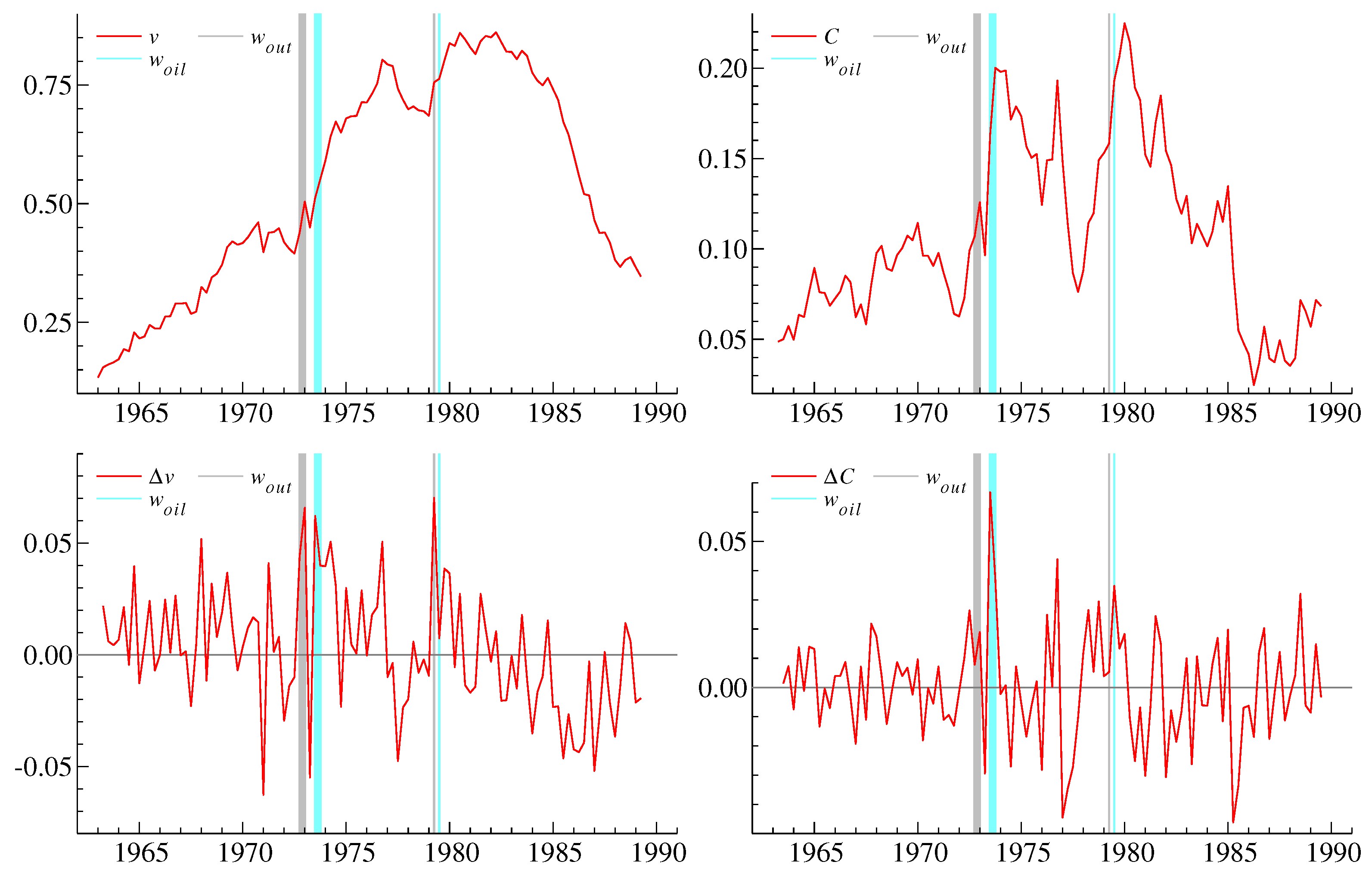
Figure 1 shows $v_t$, $C_t$ in levels and differences. The transformed data series are non-stationary, but their first-order differences have a more stationary appearance. The plots also show two dummy variables $w_{out,t}$, $w_{oil,t}$ representing large fiscal expansions in 1972:4–1973:1 and 1979:2 as well as the oil price shocks in 1973:3–4 and 1979:3. They will later be interpreted as catalysts.

Whereas the oil shocks are clearly exogenous to the UK economy, this is less obvious for the fiscal expansions. In fact, what we call fiscal shocks are the expansionary budget of 1972 proposed by Anthony Barber, then Chancellor of the Exchequer, and a significant VAT reduction in 1979. While both are likely endogenous to the UK economy, neither shock was set up to influence money demand, and so both can be considered exogenous for the bivariate model of $(v,C)$. Furthermore, while the shocks are different in principle, the effect is the same so that it becomes possible to extend our conclusions over several types of shocks that are expansionary in nature.

The dummy variables are taken from Hendry and Mizon (1993). They were originally found through a residual analysis as large outliers. By including dummies for these particular observations, the remaining observations appear to match a normal reference distribution, and the model passes standard specification tests including recursive tests. At the same time, these dummies have interpretation as interventions and are in this respect related to the historical narrative approach of Romer and Romer (2010).

The initial specification is a second-order vector autoregressive model including the two dummy variables $w_{out,t}$ and $w_{oil,t}$, that is

$$\begin{array}{ccc}\hfill \Delta v_t& =& {\pi }_{vv}{v}_{t-1}+{\pi }_{vC}{C}_{t-1}+{\psi }_{vv}\Delta v_{t-1}+{\psi }_{vC}\Delta C_{t-1}+{\mu }_v\hfill \\ & & +{\gamma }_{v,out}{w}_{out,t}+{\gamma }_{v,oil}{w}_{oil,t}+{ϵ}_{v,t},\hfill \end{array}$$

(56)

$$\begin{array}{ccc}\hfill \Delta C_t& =& {\pi }_{Cv}{v}_{t-1}+{\pi }_{CC}{C}_{t-1}+{\psi }_{Cv}\Delta v_{t-1}+{\psi }_{CC}\Delta C_{t-1}+{\mu }_C\hfill \\ & & +{\gamma }_{C,out}{w}_{out,t}+{\gamma }_{C,oil}{w}_{oil,t}+{ϵ}_{C,t}.\hfill \end{array}$$

(57)

The estimated model is the joint model reported in equilibrium-correction form in the first two columns of

Table 1. Three models estimated over the period 1963:4 to 1989:2. Standard errors reported in parentheses.

		Joint			Conditional			Structural
		Model			Models			Model
		$\Delta {\mathit{v}}_{\mathit{t}}$	$\Delta {\mathit{C}}_{\mathit{t}}$		$\Delta {\mathit{v}}_{\mathit{t}}|\Delta {\mathit{C}}_{\mathit{t}}$	$\Delta {\mathit{C}}_{\mathit{t}}|\Delta {\mathit{v}}_{\mathit{t}}$		$\Delta {\mathit{v}}_{\mathit{t}}$	$\Delta {\mathit{C}}_{\mathit{t}}$
$\Delta v_t$		–	–		–	$\underset{\left(0.075\right)}{0.433}$ *		–	$\underset{\left(0.068\right)}{0.402}$ *
$\Delta C_t$		–	–		$\underset{\left(0.104\right)}{0.606}$ *	–		$\underset{\left(0.093\right)}{0.579}$ *	−
$\Delta v_{t-1}$		$-\underset{\left(0.095\right)}{0.343}$ *	$-\underset{\left(0.081\right)}{0.048}\phantom{*}$		$-\underset{\left(0.082\right)}{0.314}$ *	$\underset{\left(0.074\right)}{0.100}\phantom{*}$		$-\underset{\left(0.091\right)}{0.317}$ *	$\underset{\left(0.076\right)}{0.092}\phantom{*}$
$\Delta C_{t-1}$		$\underset{\left(0.117\right)}{0.086}\phantom{*}$	$\underset{\left(0.099\right)}{0.046}\phantom{*}$		$\underset{\left(0.100\right)}{0.058}\phantom{*}$	$\underset{\left(0.085\right)}{0.009}\phantom{*}$		$\underset{\left(0.108\right)}{0.064}\phantom{*}$	$\underset{\left(0.090\right)}{0.003}\phantom{*}$
$v_{t-1}$		$-\underset{\left(0.014\right)}{0.097}$ *	$-\underset{\left(0.012\right)}{0.005}\phantom{*}$		$-\underset{\left(0.012\right)}{0.094}$ *	$\underset{\left(0.013\right)}{0.037}$ *		$-\underset{\left(0.012\right)}{0.095}$ *	$\underset{\left(0.013\right)}{0.035}$ *
$C_{t-1}$		$\underset{\left(0.071\right)}{0.529}$ *	$-\underset{\left(0.060\right)}{0.077}\phantom{*}$		$\underset{\left(0.062\right)}{0.575}$ *	$-\underset{\left(0.065\right)}{0.306}$ *		$\underset{\left(0.066\right)}{0.575}$ *	$-\underset{\left(0.068\right)}{0.293}$ *
1		$-\underset{\left(0.006\right)}{0.004}\phantom{*}$	$\underset{\left(0.005\right)}{0.009}\phantom{*}$		$-\underset{\left(0.005\right)}{0.009}\phantom{*}$	$\underset{\left(0.004\right)}{0.011}$ *		$-\underset{\left(0.005\right)}{0.009}\phantom{*}$	$\underset{\left(0.004\right)}{0.011}$ *
$w_{out,t}$		$\underset{\left(0.012\right)}{0.051}$ *	$\underset{\left(0.010\right)}{0.013}\phantom{*}$		$\underset{\left(0.010\right)}{0.044}$ *	$-\underset{\left(0.009\right)}{0.010}\phantom{*}$		$\underset{\left(0.010\right)}{0.039}$ *	$0\phantom{*}$
$w_{oil,t}$		$\underset{\left(0.012\right)}{0.030}$ *	$\underset{\left(0.010\right)}{0.051}$ *		$-\underset{\left(0.011\right)}{0.001}\phantom{*}$	$\underset{\left(0.009\right)}{0.038}$ *		$0\phantom{*}$	$\underset{\left(0.008\right)}{0.039}$ *
${\widehat{\sigma }}_{vv}^{1/2}$		$0.019\phantom{*}$	–		–	–		–	–
${\widehat{\sigma }}_{CC}^{1/2}$		–	$0.016\phantom{*}$		–	–		–	–
$\widehat{\rho }$		0.512			–			0.482
${\widehat{\sigma }}_{vv·C}^{1/2}$		–	–		$0.017\phantom{*}$	–		$0.016\phantom{*}$	–
${\widehat{\sigma }}_{CC·v}^{1/2}$		–	–		−	$0.014\phantom{*}$		–	$0.014\phantom{*}$
Likelihood		559.31						558.74

* indicates significance at the 5% level.

. The innovations ${ϵ}_{v,t}$, ${ϵ}_{C,t}$ are assumed i.i.d. jointly normal with zero mean and independent of the current and past regressors.

Specification tests are reported in

Table 2. Specification tests for unrestricted joint model. p-values reported in brackets.

Test	${\mathit{\chi }}_{\mathsf{norm}}^2\left[2\right]$	${\mathsf{F}}_{\mathsf{ar}(1-5)}[5,91]$	${\mathsf{F}}_{\mathsf{arch}(1-4)}[4,95]$	${\mathsf{F}}_{\mathsf{het}}[10,92]$	$max\mathit{Chow}$
$\Delta v_t$	$2.2\left[0.33\right]$	$0.4\left[0.86\right]$	$1.2\left[0.32\right]$	$0.6\left[0.81\right]$	$8.4\left[0.29\right]$
$\Delta C_t$	$1.9\left[0.39\right]$	$1.9\left[0.10\right]$	$2.1\left[0.08\right]$	$1.5\left[0.15\right]$	$12.3\left[0.04\right]$

. The residual specification tests include a cumulant based test ${\chi }_{\mathsf{norm}}^2$ for normality, a test ${\mathsf{F}}_{\mathsf{ar}}$ for autoregressive temporal dependence (Godfrey 1978), a test ${\mathsf{F}}_{\mathsf{arch}}$ for autoregressive conditional heteroscedasticity (Engle 1982), a test ${\mathsf{F}}_{\mathsf{het}}$ for heteroscedasticity (White 1980) and a test $maxChow$ based on the maximum of recursive 1-step-ahead Chow (1960) forecast test statistics. We will benefit from this recursive test in Section 6.6. The above references only consider static or stationary models, but the specification tests also apply for non-stationary autoregressions, see Kilian and Demiroglu (2000) for ${\chi }_{\mathsf{norm}}^2$, Nielsen (2006) for ${\mathsf{F}}_{\mathsf{ar}}$ and Nielsen and Whitby (2015) for $maxChow$. We see that the specification for the velocity equation is very good, while the specification for the cost equation is less good but tolerable. The two Chow tests take their maximum values in 1971:1 and in 1976:4. These dates correspond to the decimalization of the Pound and the debt intervention by the International Monetary Fund. Overall, these tests indicate that we cannot reject the model and that the innovations are independent, identically normal.

The dummy variables play a dual role in the subsequent analysis. First, we need the dummy variables to achieve a reasonable specification of the econometric model. Without these, the residuals appear too irregular and we cannot perform valid inference. The chosen statistical model is based on the normal distribution and the observations captured by the dummy variables are outliers relative to this reference distribution. Second, the dummy variables help us to distinguish between large and small shocks. The large shocks occur infrequently, and they are often interpretable as catalysts.

The above specification analysis indicates that the largest shocks after the oil crises and output expansions are the decimalization of the Pound in 1971:1 and the turmoil around the IMF intervention in 1976:4. In terms of fit, the results in Table 2 do not suggest that it is necessary to include dummies to represent these events. This could be followed up with a sensitivity analysis for the inference we draw about the oil shocks and the output expansion. For instance, does it make a difference to include a dummy for the decimalization? At the same time, we could include dummies for the decimalization and the IMF intervention to explore the transmission of those events. In other words, if we are concerned with a particular macroeconomic intervention we can to some extent search for similar interventions in the past and explore their transmission.

6.2. Causal Transmission in UK Money Demand Data

We now explore causal transmission. Table 1 reports the unrestricted reduced-form model in columns 1 and 2. This is a model for $v_t,C_t$ given dummies and the past. In the estimated model (56) and (57), we have assumed that the joint density of the innovations ${ϵ}_{v,t}$, ${ϵ}_{C,t}$ given contemporaneous and past regressors is i.i.d. zero mean jointly normal. When applying the theory of Section 3, the density $\mathsf{f}(y,z|w)$ will represent the estimated innovation density. Depending on the context, $y,z$ will refer to ${ϵ}_{v,t}$, ${ϵ}_{C,t}$ in some order, w will refer to one of the dummy variable $w_{out,t}$, $w_{oil,t}$ and the remaining regressors are ignored.

The effect of the oil price shocks can be explored by conditioning $v_t$ on $C_t$ and follow Example 2. The conditional equation for $v_t$ given $C_t$ and the marginal equation for $C_t$ are reported in columns 3 and 2, respectively, in Table 1. The coefficient for $w_{oil,t}$ is insignificant in the conditional equation but significant in the marginal equation. Theorem 1 shows there exists a unique Markov structure such that $v_t$ and $w_{oil,t}$ are conditionally independent given $C_t$. Further, the coefficient for $\Delta C_t$ is significant in the conditional equation. Theorem 2 then shows the Markov structure is non-trivial so ${\underline{w}}_{oil,t}$—$C_t$—$v_t$. Lemma 3 then shows that the transmission between $w_{oil,t}$ and $v_t$ is non-trivial. Correspondingly, the coefficient for $w_{oil,t}$ is significant in the marginal $v_t$ equation. From an economic perspective, it seems reasonable to interpret the oil shocks as catalysts so that $w_{oil,t}\to C_t\to v_t$. The interpretation is that large oil price shocks move the cost of holding money and in turn the velocity.

To illustrate the uniqueness result, we now consider the conditional equation for $C_t$ given $v_t$ in column four of Table 1. Here, $w_{oil,t}$ is significant, so we cannot have a Markov structure from $w_{oil,t}$ through $v_t$ to $C_t$. This is in line with Theorem 1.

Turning to the output shock, we condition $C_t$ on $v_t$. The conditional equation for $C_t$ given $v_t$ and the marginal equation for $v_t$ are reported in columns 4 and 1, respectively. We follow Example 2 again. The output dummy $w_{out,t}$ is significant in the marginal equation and insignificant in the conditional equation. Moreover, velocity, $\Delta v_t$, is significant in the conditional equation. Theorems 1 and 2 then show a non-trivial Markov structure ${\underline{w}}_{out,t}$—$v_t$—$C_t$. Lemma 3 shows that the transmission is non-trivial. Interpreting $w_{out,t}$ as a catalyst, we then have $w_{out,t}\to v_t\to C_t$. Economically, large fiscal expansions may impact the velocity of money without having an impact on inflation straight away. The conclusion is, however, less clear than the causal transmission of the oil shocks. Indeed, in line with the discussion in Section 3.1.3, we check if the fiscal shock $w_{out,t}$ actually has a non-negligible effect on the cost of holding money. The coefficient in the $C_t$ equation has a $\mathsf{t}$-statistic of 1.3, which at best shows marginal significance. Thus, we may very well have $w_{out,t}\to v_t\to C_t$, but evidence for this transmission is weaker than the evidence for the transmission of the oil shocks.

6.3. Imposing Multiple Catalysts

The two causal transmissions $w_{oil,t}\to C_t\to v_t$ and $w_{out,t}\to v_t\to C_t$ can be imposed individually. These are the hypotheses ${\mathsf{H}}_1$, ${\mathsf{H}}_2$ of (26) and (27). Imposing both gives as described in Section 3.3. This is a system of seemingly unrelated regressions. When maximizing the likelihood, we chose to parametrize it in terms of ${\sigma }_{yy·z}$, ${\sigma }_{zz·y}$, $\rho$ and derive standard errors for ${\gamma }_{yz}$ and ${\gamma }_{zy}$ using the $\delta$-method.

The restricted model is reported in columns 5 and 6 of Table 1 in the structural form derived from Section 3.3. The likelihood ratio statistic for the two restrictions is $2(559.31-558.74)=1.14$, which is not significant when compared to a ${\chi }_2^2$ distribution. The structural estimates largely match those of the conditional models in Table 1. Writing the model in structural form, it becomes very clear that the dummies $w_{out,t},w_{oil,t}$ affect distinct linear combinations of the endogenous variables. The first structural equation is interpretable as the monetary quantity relation, showing how money demand reacts to output shocks, while the second structural equation is interpretable as a cost-push relation showing how money demand is driven by price shocks.

6.4. Cointegration

The velocity and cost of holding money variables are non-stationary and should possibly be subjected to a cointegration analysis. This is compatible with causal transmission.

Following the maximum likelihood setup of Johansen (1995), the cointegration model with rank one is given by the equilibrium-correction model

$$\begin{array}{c}\left(\begin{array}{c}\Delta v_t\\ \Delta C_t\end{array}\right)=\left(\begin{array}{c}{\alpha }_v\\ {\alpha }_C\end{array}\right)({\beta }_v{v}_{t-1}+{\beta }_C{C}_{t-1}+{\beta }_1)\hfill \\ \hfill +\left(\begin{array}{cc}{\gamma }_{vv}& {\gamma }_{vC}\\ {\gamma }_{Cv}& {\gamma }_{CC}\end{array}\right)\left(\begin{array}{c}\Delta v_{t-1}\\ \Delta C_{t-1}\end{array}\right)+\left(\begin{array}{cc}{\gamma }_{v1}& {\gamma }_{v2}\\ {\gamma }_{C1}& {\gamma }_{C2}\end{array}\right)\left(\begin{array}{c}{w}_{out,t}\\ w_{oil,t}\end{array}\right)+\left(\begin{array}{c}{ϵ}_{v,t}\\ {ϵ}_{C,t}\end{array}\right)\end{array}$$

(58)

The model with multiple causal transmissions and cointegration imposed has a likelihood $555.44$. For present purposes, we merely consider the likelihood ratio test for the cointegration restriction within the model with multiple causal transmission imposed. The test statistic is $2(558.74-555.44)=6.60$, which should be compared to a 95% critical value of $9.1$, see Johansen (1995, Table 15.2).

With a unit cointegration rank, the coefficients to $v_{t-1}$, $C_{t-1}$ are proportional across the equations. This results in the cointegrating relation $v_{t-1}=6.239C_{t-1}$, which is interpretable as long-run money demand. The adjustment coefficient in the conditional equation for $v_t$ given $C_t$ is a modest 9.5% per quarter, whereas the adjustment in the marginal equation for $C_t$ is insignificant. We note that in a model without multiple causal transmissions imposed, the constraint ${\alpha }_C=0$ would be a hypothesis of weak exogeneity, Johansen (1995, §8), but the weak exogeneity is broken when imposing the cross-equation restrictions implied by causal transmission.

6.5. Impulse Responses

We now carry out an impulse response analysis with respect to the economic shocks represented by $w_{out,t}$ and $w_{oil,t}$. We reconstruct empirical scenarios and compare our results to the data. Thereby, the impulse responses are associated with particular shocks at particular points in time and their trajectories can be compared with the actual development of the data. This offers a distinct advantage over impulse responses created by placing identifying restrictions on the covariance matrix. Figure 2a,b explores the period around the first oil crisis, where the fiscal expansions in 1972:4–73:1 are followed by the oil shock in 1973:3–4. Likewise, Figure 2c,d explores the period around the second oil crisis, where the fiscal expansions in 1979:2 are followed by the oil shock in 1979:3. In both cases, we provide joint impulse responses and compare these to real data over a five-year horizon in Figure 2. All joint impulses perform remarkably well compared to the scenario under consideration. What is more, the impulse response functions do not decline in performance across each scenario, indicating a temporal stability in causal transmission. This is addressed further in Section 6.6.

6.6. Lucas Critique

Major shocks such as the oil crises and fiscal expansions change the policy environment and, in turn, may influence the behavior of individual agents. It has long been a concern whether this results in instability for the parameters of an economic model, rendering it useless for analyzing the effect of implementing the policy. This is known as the Lucas (1976) critique, although the concern goes back to Frisch and Haavelmo. Engle and Hendry (1993) argue that tests of super exogeneity are of interest when seeking to address the Lucas critique. Causal transmission is relevant in a similar way. We illustrate the use of causal transmission in policy analysis by performing a recursive analysis of the money data.

Previously, $w_{oil,t}$ was constructed as the sum of impulse indicators across the two oil crises. Now, we construct dummies $w_{oil1,t},w_{oil2,t}$ for 1973:3–4 and 1979:3, respectively, so that $w_{oil,t}=w_{oil1,t}+w_{oil2,t}$. We re-estimate the equations for $\left(v_t\right|C_t)$, $\left(C_t\right)$ reported in

Table 3. Estimation for UK M1 data based on a subsample and the full sample.

		1963:4–1977:2			1963:4–1989:2
		$\Delta {\mathit{v}}_{\mathit{t}}|\Delta {\mathit{C}}_{\mathit{t}}$	$\Delta {\mathit{C}}_{\mathit{t}}$		$\Delta {\mathit{v}}_{\mathit{t}}|\Delta {\mathit{C}}_{\mathit{t}}$	$\Delta {\mathit{C}}_{\mathit{t}}$
$\Delta C_t$		$\underset{\left(0.189\right)}{0.542}$ *	–		$\underset{\left(0.105\right)}{0.605}$ *	–
$\Delta v_{t-1}$		$-\underset{\left(0.123\right)}{0.359}$ *	$-\underset{\left(0.094\right)}{0.060}\phantom{*}$		$-\underset{\left(0.087\right)}{0.311}$ *	$-\underset{\left(0.084\right)}{0.031}\phantom{*}$
$\Delta C_{t-1}$		$-\underset{\left(0.185\right)}{0.004}\phantom{*}$	$-\underset{\left(0.142\right)}{0.092}\phantom{*}$		$\underset{\left(0.101\right)}{0.057}\phantom{*}$	$\underset{\left(0.099\right)}{0.036}\phantom{*}$
$v_{t-1}$		$-\underset{\left(0.032\right)}{0.097}$ *	$\underset{\left(0.025\right)}{0.007}\phantom{*}$		$-\underset{\left(0.013\right)}{0.094}$ *	$-\underset{\left(0.012\right)}{0.003}\phantom{*}$
$C_{t-1}$		$\underset{\left(0.145\right)}{0.626}$ *	$-\underset{\left(0.111\right)}{0.146}\phantom{*}$		$\underset{\left(0.063\right)}{0.574}$ *	$-\underset{\left(0.061\right)}{0.084}\phantom{*}$
1		$-\underset{\left(0.008\right)}{0.012}\phantom{*}$	$\underset{\left(0.006\right)}{0.012}$ *		$-\underset{\left(0.005\right)}{0.009}\phantom{*}$	$\underset{\left(0.005\right)}{0.009}\phantom{*}$
$w_{out,t}$		$\underset{\left(0.015\right)}{0.042}$ *	$\underset{\left(0.011\right)}{0.016}\phantom{*}$		$\underset{\left(0.010\right)}{0.044}$ *	$\underset{\left(0.010\right)}{0.013}\phantom{*}$
$w_{oil1,t}$		$\underset{\left(0.018\right)}{0.001}\phantom{*}$	$\underset{\left(0.011\right)}{0.058}$ *		$\underset{\left(0.014\right)}{0.000}\phantom{*}$	$\underset{\left(0.012\right)}{0.055}$ *
$w_{oil2,t}$		–	–		$-\underset{\left(0.018\right)}{0.002}\phantom{*}$	$\underset{\left(0.017\right)}{0.043}$ *

* indicates significance at the 5% level.

over subsamples 1963:4–1977:2 and 1963:4-1989:3 using the split oil dummy. It is clear that the transmission of the first catalyst $w_{oil1}\to C\to v$ does not differ in a statistically significant way from the transmission of the second catalyst $w_{oil2}\to C\to v$. Deconstructing the catalyst $w_{out}$ provides similar evidence for the stability of the causal transmission of the output shocks. The search for causal transmission in well-specified models therefore seems relevant when considering the Lucas critique. This does, of course, go hand in hand with the fact that the model in Table 1 passes recursive specification tests, such as the $maxChow$ test.

7. Concluding Remarks

Causal transmission has been introduced to capture the idea that large economic shocks may transmit gradually through the macroeconomy.

There are three ingredients to the definition of causal transmission of catalyst w through z to y. First, we need a non-trivial Markov structure w—z—y, that is, the Markov structure $\mathsf{f}(y,z|w)=\mathsf{f}(y\left|z\right)\mathsf{f}\left(z\right|w)$ needs to be non-trivial in the sense that $y,z$ are dependent and $z,w$ are dependent. Secondly, we need a non-trivial transmission between $w,y$ so that $w,y$ are dependent. Thirdly, we need a causal assumption for the catalyst w. When these conditions are satisfied, we write $w\to z\to y$. We have shown how this definition can be extended to the transmission of two unrelated catalysts.

Causal transmission is defined for general densities and it does not require normality. The first two conditions to the definition of causal transmission are testable using observational data. In standard models, the first condition of a non-trivial Markov structure implies the second condition of a non-trivial transmission. These standard models include normal models and mixtures of normal and logit/probit models.

Causal transmissions also require a catalyst. As in instrumental variable analysis, the catalyst can be found as a natural experiment formulated prior to the empirical analysis or it may be discoverable from the empirical analysis of observational data. Outlier detection algorithms such as Autometrics by Doornik (2009) may be helpful in this respect. The causal transmission relies on an economic interpretation of the catalyst where the narrative approach of Romer and Romer (2010) may prove helpful. Catalysts have to be statistically significant to be discoverable, and the evidence of causal transmission is stronger if found in several instances. In these ways, the empirical analysis of causal transmission is consistent with the criteria for causation in Hill (1965).

The present analysis was inspired by Bårdsen et al. (2017), who construct 3-year ahead quarterly forecasts from March 2007 generated from their macro-econometric model for Norway. In 2008, policymakers in Norway and abroad changed the policy rate dramatically in response to the financial crisis, creating a large shift of the short-term interest rate. It appears that this had the causal impact of offsetting potential big shifts in the labor market in such a way that the macro-econometric model produces good forecasts of unit labor cost, inflation and unemployment despite the financial crisis. It is plausible that the effects seen in the forecasts of the Norwegian macro-econometric models of Bårdsen et al. (2017) could be described as a combination of a major financial shock and a subsequent policy reaction calibrated to offset the financial shock in the labor market.

It would be interesting to develop the ideas on causal transmission in larger statistical models of the economy. First, to what extent does a causal transmission analysis of $\mathsf{f}(y,z|w)$ extend to $\mathsf{f}(x,y,z|w)$? Second, where interventions can be identified as catalysts that induce a particular dependence structure or causal transmission among modeled variables, these can be deployed out of sample to attenuate adverse shocks by targeting dependence chains, as opposed to single variables.

References

- Andersson, Steen A., David Madigan, and Michael D. Perlman. 2001. Alternative Markov properties for chain graphs. Scandinavian Journal of Statistics 28: 33–85. [Google Scholar] [CrossRef]
- Angrist, Joshua D., Kathryn Graddy, and Guido W. Imbens. 2000. The interpretation of instrumental variables estimators in simultaneous equations models with an application to the demand for fish. Review of Economic Studies 67: 499–527. [Google Scholar] [CrossRef]
- Bårdsen Gunnar, Dag Kolsrud, and Ragnar Nymoen. 2017. Forecasting robustness in macroeconometric models. Journal of Forecasting 36: 629–39. [Google Scholar] [CrossRef]
- Birch, M. W. 1963. Maximum likelihood in three-way contingency tables. Journal of the Royal Statistical Society. Series B 25: 220–33. [Google Scholar] [CrossRef]
- Cartwright, Nancy. 1989. Nature’s Capacities and Their Measurement. Oxford: Clarendon Press. [Google Scholar]
- Centoni, Marco, and Gianluca Cubadda. 2015. Common feature analysis of economic time series: An overview and recent developments. Communications for Statistical Applications and Methods 22: 415–34. [Google Scholar] [CrossRef] [Green Version]
- Chow, Gregory C. 1960. Tests of equality between sets of coefficients in two linear regressions. Econometrica 28: 591–605. [Google Scholar] [CrossRef]
- Cloyne, James. 2013. Discretionary tax changes and the macroeconomy: New narrative evidence from the United Kingdom. American Economic Review 103: 1507–28. [Google Scholar] [CrossRef] [Green Version]
- Cox, David, and Nanny Wermuth. 2003. A general condition for avoiding effect reversal after marginalization. Journal of the Royal Statistical Society Series B 65: 937–41. [Google Scholar] [CrossRef]
- Cox, David, and Nanny Wermuth. 2004. Causality: A statistical view. International Statistical Review 72: 285–305. [Google Scholar] [CrossRef]
- Dawid, A. Philip. 1979. Conditional independence in statistical theory (with discussion). Journal of the Royal Statistical Society. Series B 41: 1–31. [Google Scholar]
- Dawid, A. Philip. 1980. Conditional independence for statistical operations. Annals of Statistics 8: 598–617. [Google Scholar] [CrossRef]
- Doornik, Jurgen A. 2009. Autometrics. In The Methodology and Practice of Econometrics: Festschrift in Honour of David F. Hendry. Edited by Jennifer L. Castle and Neil Shephard. Oxford: Oxford University Press, pp. 88–121. [Google Scholar]
- Doornik, Jurgen A., and David F. Hendry. 2013. PcGive 14. London: Timberlake, vol. 2. [Google Scholar]
- Drton, Mathias. 2009. Discrete chain graph models. Bernoulli 15: 736–53. [Google Scholar] [CrossRef]
- Drton, Mathias, and Thomas S. Richardson. 2004. Multimodality of the likelihood in the bivariate seemingly unrelated regressions model. Biometrika 91: 383–92. [Google Scholar] [CrossRef]
- Engle, Robert F. 1982. Autoregressive conditional heteroscedasticity with estimates of the variance of United Kingdom inflation. Econometrica 50: 987–1108. [Google Scholar] [CrossRef]
- Engle, Robert F., and David F. Hendry. 1993. Testing superexogeneity and invariance in regression models. Journal of Econometrics 56: 119–39. [Google Scholar] [CrossRef]
- Engle, Robert F., David F. Hendry, and Jean-Francois Richard. 1983. Exogeneity. Econometrica 51: 277–304. [Google Scholar] [CrossRef]
- Engle, Robert F., and Sharon Kozicki. 1993. Testing for common features. Journal of Business & Economic Statistics 11: 369–80. [Google Scholar]
- Fallat, Shaun, Steffen Lauritzen, Kayvan Sadeghi, Caroline Uhler, Nanny Wermuth, and Piotr Zwiernik. 2017. Total positivity in Markov structures. Annals of Statistics 45: 1152–84. [Google Scholar] [CrossRef] [Green Version]
- Fisher, R. A. 1922. On the interpretation of χ2 from contingency tables, and the calculation of p. Journal of the Royal Statistical Society 85: 87–94. [Google Scholar] [CrossRef]
- Frydenberg, Morten. 1990. The chain graph Markov property. Scandinavian Journal of Statistics 17: 333–53. [Google Scholar]
- Godfrey, Leslie G. 1978. Testing against general autoregressive and moving average error models when the regressors include lagged dependent variables. Econometrica 46: 1293–301. [Google Scholar] [CrossRef]
- Graddy, Kathryn. 1995. Testing for imperfect competition at the Fulton Fish Market. RAND Journal of Economics 26: 75–92. [Google Scholar] [CrossRef]
- Granger, Clive W. J. 1969. Investigating causal relations by econometric models and cross-spectral methods. Econometrica 37: 424–38. [Google Scholar] [CrossRef]
- Hendry, David F. 1995. Dynamic Econometrics. Oxford: Oxford University Press. [Google Scholar]
- Hendry, David F. 1999. An econometric analysis of US food expenditure, 1931–1989. In Methodology and Tacit Knowledge: Two Experiments in Econometrics. Edited by Jan R. Magnus and Mary S. Morgan. New York: John Wiley & Sons, pp. 341–61. [Google Scholar]
- Hendry, David F., and Jurgen A. Doornik. 2014. Empirical Model Discovery and Theory Evaluation: Automatic Selection Methods in Econometrics. London: MIT Press. [Google Scholar]
- Hendry, David F., and Neil R. Ericsson. 1991. An econometric analysis of U.K. money demand in Monetary Trends in the United States and the United Kingdom by Milton Freedman and Anna J. Schwartz. American Economic Review 81: 8–38. [Google Scholar]
- Hendry, David F., Søren Johansen, and Carlos Santos. 2008. Automatic selection of indicators in fully saturated regression. Computational Statistics 23: 317–35, Erratum ibid. pp. 337–339. [Google Scholar] [CrossRef] [Green Version]
- Hendry, David F., and Michael Massmann. 2007. Co-breaking: Recent advances and a synopsis of the literature. Journal of Business & Economic Statistics 25: 33–51. [Google Scholar]
- Hendry, David F., and Grayham E. Mizon. 1993. Evaluating dynamic econometric models by encompassing the VAR. In Models, Methods and Applications of Econometrics. Edited by Peter C. B. Phillips. Oxford: Blackwell, pp. 272–300. [Google Scholar]
- Hendry, David F., and Bent Nielsen. 2007. Econometric Modeling: A Likelihood Approach. Princeton: Princeton University Press. [Google Scholar]
- Hendry, David F., and Carlos Santos. 2010. An automatic test of super exogeneity. In Volatility and Time Series Econometrics: Essays in Honor of Robert F. Engle. Edited by Tim Bollerslev, Jeffrey R. Russell and Mark W. Watson. Oxford: Oxford University Press. [Google Scholar]
- Hill, Austin Bradford. 1965. The environment and disease: Association or causation? Proceedings of the Royal Society of Medicine 58: 295–300. [Google Scholar] [CrossRef] [Green Version]
- Imbens, Guido W. 2014. Instrumental variables: An econometrician’s perspective. Statistical Science 29: 323–58. [Google Scholar] [CrossRef]
- Johansen, Søren. 1995. Likelihood Based Inference on Cointegration in the Vector Autoregressive Model. Oxford: Oxford University Press. [Google Scholar]
- Johansen, Søren, and Bent Nielsen. 2009. Saturation by indicators in regression models. In The Methodology and Practice of Econometrics: Festschrift in Honour of David F. Hendry. Edited by Jennifer L. Castle and Neil Shephard. Oxford: Oxford University Press, pp. 1–36. [Google Scholar]
- Johansen, Søren, and Bent Nielsen. 2016. Asymptotic theory of outlier detection algorithms for linear time series regression models (with discussion). Scandinavian Journal of Statistics 43: 321–81. [Google Scholar] [CrossRef] [Green Version]
- Kilian, Lutz, and Ufuk Demiroglu. 2000. Residual-based tests for normality in autoregressions: Asymptotic theory and simulation evidence. Journal of Business & Economic Statistics 18: 40–50. [Google Scholar]
- Lauritzen, Steffen L. 1996. Graphical Models. Oxford: Oxford University Press. [Google Scholar]
- Lauritzen, Steffen L., and Nanny Wermuth. 1989. Graphical models for associations between variables, some of which are qualitative and some quantitative. Annals of Statistics 17: 31–57. [Google Scholar] [CrossRef]
- Lucas, Robert E. 1976. Econometric policy evaluation: A critique. In Theory, Policy, Institution: Papers from the Carnegie-Rochester Conference Series on Public Policy. Edited by Karl Brunner and Allan Meltzer. Amsterdam: Elsevier, pp. 19–46. [Google Scholar]
- MATLAB. 2014. Version 8.4.0 (R2014b). Natick: The MathWorks Inc. [Google Scholar]
- Montiel Olea, José L., James H. Stock, and Mark W. Watson. 2021. Inference in structural vector autoregressions identified with external instruments. Journal of Econometrics 225: 74–87. [Google Scholar] [CrossRef]
- Nielsen, Bent. 2006. Order determination in general vector autoregressions. In Time Series and Related Topics: In Memory of Ching-Zong Wei. Edited by Hwai Chung Ho, Ching Kang Ing and Tze Leung Lai. Volume 52 of Lecture Notes–Monograph Series; Beachwood: Institute of Mathematical Statistics, pp. 93–112. [Google Scholar]
- Nielsen, Bent, and Andrew Whitby. 2015. A joint Chow test for structural instability. Econometrics 3: 156–86. [Google Scholar] [CrossRef] [Green Version]
- Pearl, Judea. 2000. Causality: Models, Reasoning, and Inference. Cambridge: Cambridge University Press. [Google Scholar]
- Romer, Christina D., and David H. Romer. 2010. The macroeconomic effects of tax changes: Estimates based on a new measure of fiscal shocks. American Economic Review 100: 763–801. [Google Scholar] [CrossRef] [Green Version]
- Simpson, E. H. 1951. The interpretation of interaction in contingency tables. Journal of the Royal Statistical Society Series B 23: 238–41. [Google Scholar] [CrossRef]
- Sims, Christopher A. 1980. Macroeconomics and reality. Econometrica 48: 1–48. [Google Scholar] [CrossRef] [Green Version]
- Spirtes, Peter, Clark Glymour, and Richard Scheines. 2000. Causation, Prediction, and Search, 2nd ed. Cambridge: MIT Press. [Google Scholar]
- Sundberg, Rolf. 2019. Statistical Modelling by Exponential Families. Cambridge: Cambridge University Press. [Google Scholar]
- Vahid, Farshid, and Robert F. Engle. 1993. Common trends and common cycles. Journal of Applied Econometrics 8: 341–60. [Google Scholar]
- van Garderen, Kees Jan. 1997. Curved exponential models in econometrics. Econometric Theory 13: 771–90. [Google Scholar] [CrossRef]
- Wermuth, Nanny. 2012. Traceable regressions. International Statistical Review 80: 415–38. [Google Scholar] [CrossRef]
- Wermuth, Nanny, and Kayvan Sadeghi. 2012. Sequences of regressions and their independences. Test 21: 215–52. [Google Scholar] [CrossRef] [Green Version]
- White, Halbert. 1980. A heteroskedasticity-consistent covariance matrix estimator and a direct test for heteroskedasticity. Econometrica 48: 817–38. [Google Scholar] [CrossRef]
Figure 1.
Levels and first-differences of the variables in the system plotted with the selected outliers .
Figure 2.
Impulse responses matched with the data for the early and late 1970s output and oil shocks. Panels (a,b) consider the period after the first episode. Panels (c,d) consider the period after the second episode. Panels (a,c) show impulse response for v. Panels (b,d) show impulse response for C. Dashed lines are simulated 90% confidence bands.