
Global Solar Radiation and Its Interactions with Atmospheric Substances and Their Effects on Air Temperature Change in Ankara Province


1
Key Laboratory for Middle Atmosphere and Global Environment Observation (LAGEO), Institute of Atmospheric Physics, Chinese Academy of Sciences, Beijing 100029, China
2
TUBITAK Marmara Research Center, Polar Research Institute, Gebze 41470, Kocaeli, Türkiye
*
Author to whom correspondence should be addressed.
Climate 2024, 12(3), 35; https://doi.org/10.3390/cli12030035
Submission received: 12 January 2024
/
Revised: 26 February 2024
/
Accepted: 27 February 2024
/
Published: 1 March 2024
Abstract
:On the analysis of solar radiation and meteorological variables measured in Ankara province in Türkiye from 2017 to 2018, an empirical model of global solar radiation was developed. The global solar radiation at the ground and at the top of the atmosphere (TOA) was calculated and in good agreement with the observations. This model was applied to compute the losses of global solar radiation in the atmosphere and the contributions by atmospheric absorbing and scattering substances. The loss of global solar radiation in the atmosphere was dominated by the absorbing substances. The sensitivity test showed that global solar radiation was more sensitive to changes in scattering (described by a scattering factor S/G, S and G are diffuse and global solar radiation, respectively) than to changes in absorption. This empirical model was applied to calculate the albedos at the TOA and the surface. In 2017, 2018, and 2019, the computed albedos were 28.8%, 27.8%, and 28.2% at the TOA and 21.6%, 22.1%, and 21.9% at the surface, which were in reasonable agreement with satellite retrievals. The empirical model is a useful tool for studying global solar radiation and the multiple interactions between solar energy and atmospheric substances. The comparisons of global solar radiation and its loss in the atmosphere, as well as meteorological parameters, were made at some representative sites on the Earth. Some internal relationships (between G and the absorbing and scattering substances, air temperature and atmospheric substances, air temperature increase and latitude, etc.) were found. Thus, it is suggested to thoroughly study solar radiation, atmospheric substances, and climate change as a whole system and reduce the direct emissions of all atmospheric substances and, subsequently, secondary products (e.g., CO2 and non-CO2) in the atmosphere for the achievement of slowing down climate warming.
1. Introduction
Solar radiation is an important energy source to the Earth’s system and controls the variations in atmospheric constituents (NO2, SO2, O3, thousands of biogenic volatile organic compounds (BVOCs), aerosols, etc.) and meteorological parameters (air temperature, humidity, etc.) from the hourly to inter-annual time scales [1,2,3]. Solar radiation transfers into the atmosphere and interacts with the atmospheric gases, liquids, and particles (GLPs, e.g., molecules (NO2, SO2, O3, isoprene, monoterpenes, aromatic VOCs, oxygenic VOCs, water vapor, etc.), particles, and clouds). Solar radiation warms the atmosphere via the absorption and scattering processes by GLPs and reflects at the top of the atmosphere (TOA) and the surface, thus influencing the horizontal and vertical movements of the atmosphere and regional energy balance. So, it is necessary to thoroughly study (1) the transfer and loss of global solar radiation in the atmosphere, (2) the reflections at the TOA and the surface, (3) the interactions between global solar radiation, atmospheric GLPs, and meteorological variables, and (4) the mechanisms of physical and chemical processes associating with the movement of the atmosphere, the Earth’s energy balance, and climate warming [4,5,6,7,8,9,10,11].
Sophisticated radiative transfer models (LOWTRAN, MODTRAN, etc.) are widely used for the studies of solar radiation and climate change, but a large quantity of atmospheric variables (gases, aerosols, clouds, etc.), hypotheses, and parameterizations are used. Then, the empirical models are developed to estimate global, direct, and diffuse solar radiation at the surface [12,13,14,15,16,17,18,19,20,21,22,23] using fewer variables easily obtained from solar radiation and meteorological stations and the relationships between radiation and parameters (air temperature, relative humidity, sunshine duration, atmospheric transmittance, aerosol optical depth, etc.). In hybrid models developed for 12 cities in Türkiye, including Ankara, the amount of diffuse radiation was estimated with the help of meteorological parameters, and verification was achieved with a regression coefficient as high as 0.99 R2 [24]. By classifying diffuse radiation models into four groups, diffuse radiation values of Türkiye’s three largest provinces (Ankara, Istanbul, and Izmir) according to population were estimated. The estimated values in the study were obtained with an accuracy of 1.0 R2 [25]. To study the regional climate and climate change, it is not enough to study solar radiation only at the ground; that in the atmosphere and at the top of the atmosphere (TOA) is also in urgent need. This challenging task may be achieved by using a newly developed empirical model of global solar radiation with the considerations of physical and chemical mechanisms via OH radicals, H2O, NO2* (excited NO2), volatile organic compounds (VOCs, including anthropogenic VOCs (AVOCs) and BVOCs), etc., and the use of fewer variables and assumptions [26]. To fully understand the atmospheric movement, energy budget, and climate change, we should study solar radiation not only at the ground but also in the atmosphere and at the TOA, the reflection and/or albedo at TOA and at the surface, as well as the extinction of solar radiation in the atmosphere due to absorption and scattering [27].
To fully study global solar radiation (e.g., transfers in the atmosphere and reflects at the TOA and the surface) and its influences on regional climate change, the objectives of this study were to develop an empirical model of global solar radiation in Ankara province and investigate (1) global solar radiation at the ground and at the TOA, (2) the losses of global solar radiation in the atmosphere caused by the atmospheric absorbing and scattering substances, (3) the albedos at the TOA and the surface, and (4) the interactions between the global solar radiation and its losses, and absorbing and scattering GLPs. The important issue was to deeply understand the internal laws and mechanisms associated with solar radiation, atmospheric substances, and climate change. Firstly, two years of observations of solar radiation and meteorological variables in Ankara province in Türkiye were used to develop an empirical model of global solar radiation, as described in Section 2. Then, this empirical model was applied to achieve the above aims 1–4 using the observed and estimated global solar radiation in 2017–2019, and the results were compared with those from the other three typical sites of the Earth in Section 3 and Section 4 for a thorough investigating some common interaction laws between solar radiation and atmospheric substances, and meteorological parameters.
2. Data and Methodology
2.1. Observations and Data Selection
Solar radiation and meteorological parameters were measured in Ankara province (39°58′21.7″ N, 32°51′49.3″ E, elevation 890 m), Türkiye, from 1 January 2017 to 31 December 2019. Global horizontal irradiance (namely total solar irradiance on a horizontal plane, described as G, 200–3600 nm) and direct normal irradiance (described as D, 200–4000 nm) were measured with a frequency of 1 Hz using radiometers. Diffuse horizontal irradiance (described as S, 200–4000 nm) was calculated using S = G − D × cos(SZA), where SZA is the solar zenith angle (degree). Global and diffuse solar irradiance was measured by Spectrally Flat Class A un-shadowed and shadowed pyranometers (CM 22, Kipp&Zonen, Delft, The Netherlands). Direct beam irradiance was measured by a pyrheliometer (CH1, Kipp & Zonen Inc., Delft, The Netherlands). Meteorological parameters (temperature T and relative humidity RH) near the surface were measured using HMP155 sensor Pt100RD and 180R (Vaisala Inc., Vantaa, Finland), respectively. All solar radiation and meteorological data in 2017–2019 were obtained from the Turkish State Meteorology Service (TSMS).
In total, 12,681 hourly observational radiation data (daytime) were available from the Ankara province station between 1 January 2017 and 31 December 2019.
To understand variation characteristics of solar radiation in Ankara province under all sky conditions (cloudiness is from 0 to 1), all observed solar radiation data in 2017–2019 were used to calculate the daily, monthly, and annual values. Values for global and direct solar radiation larger than extraterrestrial radiation were not found. The extreme values of solar radiation (G, S, and D) and the ratio S/G (dimensionless) were excluded. We used data criteria that the measured solar radiation was in the range of 0–1.2 times the extraterrestrial radiation [28].
2.2. Development of Empirical Model of Global Solar Radiation
It should be noted that the methodology applied in this study is the same implemented at some sites in China, especially in Qianyanzhou [26]. Global solar radiation (namely total solar radiation on a horizontal plane) transfers in the atmosphere and is attenuated by GLPs. The principle of solar radiation balance was further applied to Ankara province from Qianyanzhou station (26°44′48″ N, 115°04′13″ E, elevation 110.8 m) in China, as well as four stations in North China in the UV and visible (VIS) regions (290–400, 400–700 nm) [26,28,29,30,31,32,33,34,35]. Briefly, considering the transfer processes of global solar radiation, two significant processes were taken into account:
1. Absorption (and absorption term): direct absorption and indirect consumption of global solar radiation by GLPs when they are participating in complicated chemical and photochemical reactions (CPRs), especially thousands of BVOCs (many of them are highly reactive chemical compounds) react with H2O, OH radicals (e.g., GLPs + OH + H2O + VOCs + O3 in the UV region) and NO2* (in the visible region), as well as H2O (an important absorber) in the near-infrared region (NIR) [26,29,30,31,32,33,34,35].
The global solar radiation absorbed by water vapor (0.70–2.845 μm) was computed using ΔS’ = 0.172 (mW)0.303 [36], W = 0.021E × 60 (E is the mean water vapor pressure at the Earth’s surface, hPa), and = 1 − ΔS’/Io. Where the solar constant Io = 1.94 cal min−1cm−2 (1367 W m−2), k is the mean absorption coefficient of water vapor (0.70–2.845 μm), and m is the optical air mass. The absorption term at the horizontal plane is described as × cos(SZA).
2. Scattering (and scattering term): scattering of global solar radiation by GLPs, described as e−S/G, where S/G is a normalized parameter that represents the total scattering by atmospheric substances [31].
The hourly global solar radiation under all sky conditions was computed by an empirical model:
where the subscripts cal and obs represent the calculated and observed hourly values of G (MJ m−2, 1 kWh m−2 = 3.6 MJ m−2). Coefficients A1 and A2 (MJ m−2) represent the individual G at the TOA corresponding to the absorption and scattering GLPs, respectively, based on the Lamber-Beer’s law, and A0 (MJ m−2) describes the reflection of G at the TOA. The summation of A1, A2, and A0 is the global solar radiation at the TOA. The realistic energy relationships between the absorption and scattering substances (i.e., A1 and A2) and Gobs under all sky conditions were quantified by fitting the Gobs, absorption, and scattering terms (Equation (1)).
Gcal = A1e−kWm × cos(SZA) + A2e−S/Gobs + A0
2.3. Development and Validation of the Empirical Model of Global Solar Radiation
To determine the model coefficients Ai, high-quality observed data were used with more strict criteria: SZA > 75° and G ≥ 50 W m−2 in order to reduce the influence of larger measurement errors during the early morning and late afternoon [37]. Hourly averaged solar radiation and meteorological parameters (T, RH, and E) were used to calculate daily averages, which were then computed for monthly mean values. Finally, 6160 hourly data sets (sample number n = 6160, from 2017 to 2018) were selected for empirical model development of global solar radiation (Equation (1)). The total sample number of the observed solar radiation in 2017–2018 was 8458, i.e., the remaining data number was 2298.
The coefficients Ai in Equation (1) were obtained using a multi-parameter fit to the observed hourly averages (Figure 1). The results are shown in Table 1, i.e., the coefficients (A1, A2, and A0) in Equation (1), the coefficient of determination (R2), and the mean absolute value of relative error () between calculated and observed G. The mean absolute deviations (MAD, in exposure unit, MJ m−2 and in percentage of mean observational value, %) and the root mean square errors (RMSE, in exposure unit and in percentage of mean observational value) are also reported in Table 1. Figure 2a shows the calculated and observed hourly G (Gcal and Gobs) and their relative errors (δ), and Figure 2b shows a scatter plot of the hourly Gcal versus the hourly Gobs (n = 6160). The slope of the linear regression of Gcal on Gobs is 0.9157, with a coefficient of determination (R2) of 0.9157 (confidence level α = 0.001). The results in Figure 2 and Table 1 show that the calculated G is in reasonable agreement with the observations under all sky conditions, with = 27.14%, normalized mean square error (NMSE) = 0.025 MJ m−2, MAD (MJ m−2, %) = 0.199, 11.38%, RMSE (MJ m−2, %) = 0.265, 15.14%. The standard deviation of Gcal (0.914 MJ m−2) was smaller than that of Gobs (0.955 MJ m−2). For a comparison, all the above corresponding values were larger in Ankara than that in Qianyanzhou [26]. The standard deviations of Gcal and Gobs in Ankara province were also larger than those in Qianyanzhou (σcal = 0.32, σobs = 0.39 MJ m−2 for S/G < 0.80 conditions), resulting in larger estimation biases (e.g., , MAD and RMSE). The results in Figure 2b (left bottom part) showed that there were some data points with lower Gobs than Gcal, which were caused by the following situations: (1) S/G was large (>0.8), and most of them were 1, due to clouds, aerosols, rain, etc.; (2) in the early morning (e.g., before 10:00, water vapor condenses on the surface of the sensors, foggy) and late afternoon together with long optical air mass. These reasons caused large errors in both the measurements and the model simulations [12,15,16,18,20,26]. To improve the empirical model performance for high GLP load conditions (e.g., S/G > 0.8, large cloud amount, severe air pollution, rain, sandstorm), a specific empirical model is recommended to be developed for this situation according to the study [26].
The albedo (the ratio between the upward/reflected solar radiation and the download solar radiation) at the TOA from 2017 to 2018 (A0/(A1 + A2)) was calculated using the empirical model and was 30.67%, which was a little larger than that 29.00% under all sky conditions at Qianyanzhou station in 2013–2016 [26]. The average S/G of 0.469 in Ankara province was smaller than that of 0.83 under all sky conditions at Qianyanzhou. It was probably revealed that the less atmospheric substances (e.g., S/G) together with larger land surface reflection [38] (~20% vegetation coverage) in the Ankara province region caused a slightly larger reflection of G at the TOA. Figure 2c demonstrates a scatter plot of the calculated monthly Gcal versus Gobs values (n = 24) for a thorough understanding of the estimations of monthly G.
There were strong correlations between Gobs and the absorption term (correlation coefficient R = 0.736, n = 6160) and Gobs and the scattering term (R = 0.746, n = 6160). A weak correlation existed between the absorption term and the scattering term (R = 0.199, n = 6160).
The value of the RMSE (0.265, Table 1) was in reasonable agreement with the average RMSE (0.222) estimated using 7 empirical models with better performance out of 105 models [20], meaning this empirical model is reliable.
To thoroughly investigate and validate the empirical model, more observational data were selected, i.e., hourly global solar radiation from 1 January 2017 to 31 December 2019 under all sky conditions was estimated using observed solar radiation and meteorological variables during the daytime. Table 2 reports the main calculation results of annual averages of hourly values. All estimation errors in 2019 were increased compared to that in model development (n = 6160). It is reasonable because the observed G was much lower under all sky conditions compared to that in model development (higher observed G, SZA >75° and G ≥ 50 W m−2), especially in early morning and late afternoon with large measurement errors (e.g., cosine error at low solar elevation angle). The RMSE values of 0.327 MJ m−2 and 24.82% can be acceptable for the estimations of G under all sky conditions. Similarly, the estimation errors in 2017–2019 (n = 12,681) were a little smaller than that in 2019 (n = 4323), indicating that the increase in sample number can reduce the errors in estimations (e.g., δavg, MAD, RMSE in Table 2) of G. It should be noted that there were some observations Gobs < 50 W m−2 (n = 2087) with a ratio of 16.5% in the total sample number in 2017–2019 (n = 12,681). The results from 2019 can be used as a validation of the empirical model. To thoroughly understand the basic atmospheric status and its important variables, the averages of E and S/G in 2017–2019 were reported as 8.84 hPa and 0.56, respectively. The R2 values were 0.957 (α= 0.001) and 0.959 (α= 0.001) for 2019 and 2017–2019, respectively.
3. Results
3.1. Variations in Global Solar Radiation and Their Losses in the Atmosphere
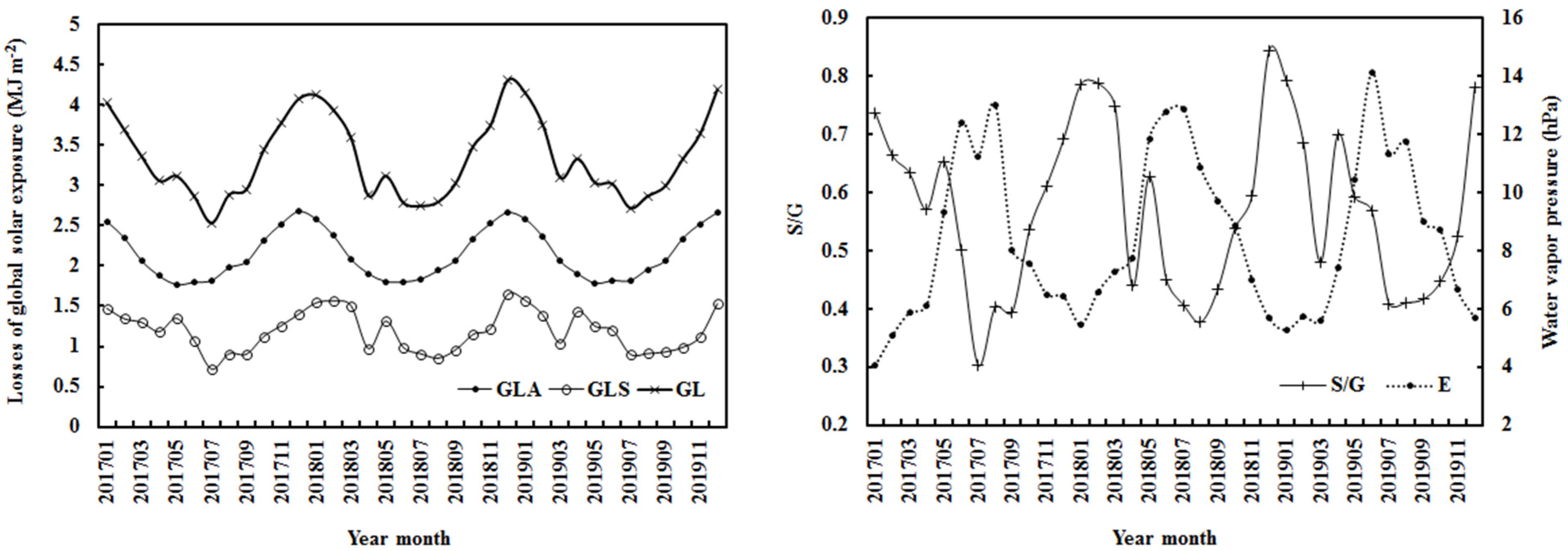
Under all sky conditions, monthly mean global solar radiation along with the absorbing and scattering losses (GLA and GLS) caused by atmospheric GLPs were calculated using A1(1 − e−kWm × cos(Z)) and A2(1 − e−S/G), respectively. The total loss GL = GLA + GLS. Figure 3 shows the calculated and observed monthly averages of G, together with S/G, from 1 January 2017 to December 2019. The empirical model of G showed a reasonable performance, and most of the estimates were within one standard deviation of Gobs. In more detail, larger relative errors of the estimations appeared in the conditions of high S/G (high GLP loads, including clouds, aerosols, dust, and air pollutants), and it was caused by the enhanced observational and calculation errors during these conditions. Thus, more studies should be carried out to reduce simulation errors under high GLP loads in the future [21].
The annual averages of the observed and calculated G in 2017–2019 decreased by −0.1% and −1.0% per year, respectively, and the increases in atmospheric GLPs (E and S/G), the key driving factors of G, were the main causes. A similar study reported that “increasing aerosol loading is responsible for the observed reduced global solar radiation” [39]. Thus, the decrease in G would result in a “solar dimming” in this region; a similar phenomenon was also found in Qianyanzhou station [26] and Jiangxi province in China from 2008 to 2016 [39].
Figure 4 shows the monthly mean losses of the global solar radiation due to atmospheric substances and their influencing factors (E and S/G) from 1 January 2017 to December 2019. The absorption losses (GLA) caused by GLP absorption dominated the total loss and showed evident variations, higher during November–January and lower during June–September, corresponding to the lower water vapor pressure (probably together with other higher GLPs, NOx, SO2, O3, particulate material, etc., similar to other sites in North China) [3] in winter and higher water vapor pressure in summer. The scattering losses (GLS) caused by GLPs’ scattering exhibited similar variations with that of GLA corresponded to similar variations in S/G (i.e., S/G lower in summer and higher in winter).
From 1 January 2017 to December 2019, GLA increased by 0.18% per year, associated with the increase in E by 3.2% per year. This was mainly contributed by the increase in absorbing substances, e.g., gases and aerosols (O3 and secondary organic aerosols (SOA)) in the UV, VIS, and NIR regions were produced from VOCs (AVOCs and BVOCs) and OH radicals when taking part in CPRs [3,26,29,31,32,33,34,35,37,40,41,42,43,44,45]. For Ankara province, the vegetation coverage is approximately 10–20% [38,46]. GLS increased by 0.8% per year, associated with the increase in S/G by 0.8% per year. GL increased by 0.4% per year. It is evident that the increases in both the absorbing and the scattering substances led to the increases in absorbing and scattering losses of G in the atmosphere. Furthermore, they resulted in the increase in annual mean air temperature (i.e., warming) during daytime by 0.13% (corresponding to 0.03 °C).
The monthly contributions of the absorbing losses to the total loss (RLA) generally appeared high values from July to November and were much larger than that of scattering loss (RLS) by about 31.1% in 2017–2019. The annual averages of RLA and RLS were 65.6% and 34.3%, respectively. It revealed that the absorbing components played predominant roles in not only total atmospheric substances but also loss of G in the Ankara province region.
The annual averages of RLA (65.6%) in the Ankara province from 2017 to 2019 was smaller than that of 79.9% at S/G < 0.80 and 93.2% at S/G ≥ 0.80 in the Qianyanzhou over 2013–2016 [26], implying that there were more absorbing GLPs in Qianyanzhou than Ankara province.
3.2. Seasonal Variations in Global Solar Radiation and the Losses in the Atmosphere
Seasonal mean losses of G caused by the absorbing and scattering GLPs from 2017 to 2019 are displayed in Figure 5 and Table 3, together with the seasonal averages of E and S/G. The contributions of the absorbing and scattering losses to the total loss are also presented in Table 3, along with the annual averages of all the above variables. GLA, GLS, GL, and S/G showed similar seasonal variations, higher in winter and lower in summer, while E displayed different seasonal variations from S/G, i.e., higher in summer and lower in winter. RLA exhibited clear seasonal variations, higher in summer and autumn and lower in spring and winter, whereas RLS exhibited inverse seasonal variations with RLA, higher in spring and winter and lower in summer and autumn.
The extinction of global solar radiation over the Ankara province was mostly dominated by absorbing compositions in four seasons. In contrast, the scattering compositions played secondary roles in the attenuation of G.
3.3. Sensitivity Analysis
The response of global solar radiation to changes in the absorbing or scattering substances (represented by E and S/G, respectively), while keeping other factors at their original levels, was computed using the empirical model (Equation (1), n = 6160). The results are shown in Figure 6 and Table 4.
The calculated hourly G at the ground decreased/increased with the increase/decrease in E, demonstrating that the increase in absorbing substances leads to enhanced losses of G in the atmosphere and the decreased G at the ground. Gcal increased/decreased with the decrease/increase in S/G, indicating that the increase in scattering substances results in a large attenuation of G. Gcal was much more sensitive to changes in the scattering factor (S/G) than the absorbing factor (E), displaying that much more scattering energy was lost in the atmosphere than absorption energy (at a low E of 8.90 hPa, n = 6160). The responses of G (ΔG) to the changes in both E (ΔE) and S/G (Δ(S/G)) were non-linear, ΔG = −9.647ln(ΔE) + 14.642 (R² = 0.984, α = 0.001), ΔG = −58.5ln(Δ(S/G)) + 88.458, (R² = 0.9784, α = 0.001).
3.4. Relationships between Wind Speed and Atmospheric GLPs (S/G)
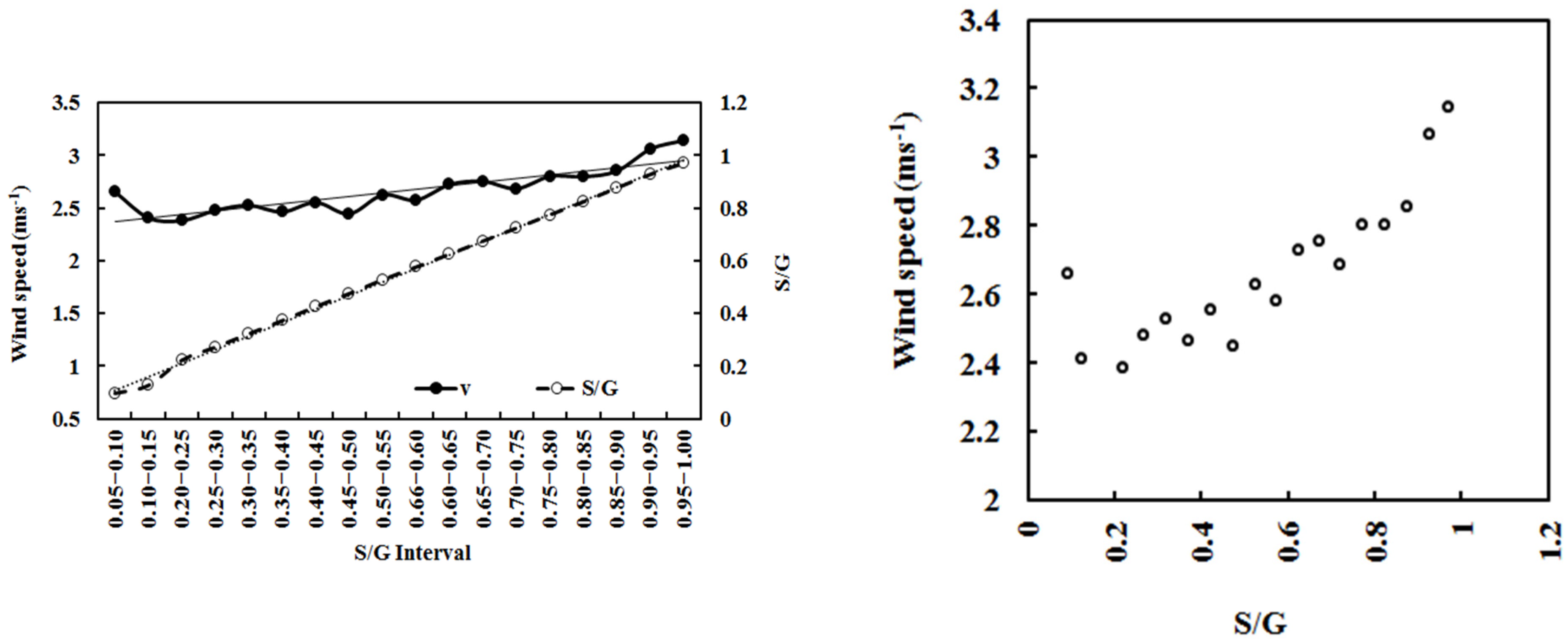
Figure 7 shows the averages of hourly wind speed and hourly atmospheric substances (S/G with an interval of 0.05 ranging from 0.00 to 1.00) from January 2017 to December 2019. A strong positive correlation was found between wind speed and S/G, v = 0.6675(S/G) + 2.2988 (R² = 0.729). A similar positive correlation between v and S/G was also found at Dome C [47], while negative correlations were exhibited between v and S/G at Qianyanzhou and Sodankylä stations [48]. The values of S/G and E were lower in Ankara and Dome C than in Qianyanzhou and Sodankylä (e.g., Table 5, Section 4.3). These relations are useful for understanding the basic characteristics of the atmosphere at different sites. It can be noticed that Qianyanzhou and Sodankylä are located in the forest regions; the heavier the atmosphere (S/G), the lower the wind speed, indicating that forests play significant roles in reducing atmospheric horizontal movement. In the non-forest regions (i.e., Dome C with a large area of flat surface and Ankara province with large gaps between small areas in the city), the heavier the atmosphere, the larger the wind speed, indicating that atmosphere gravity plays a vital role in the formation of wind.
Clear negative relationships existed for wind speed (v) versus air pressure (p), p versus S/G, v versus S/G at different S/G intervals of 0.05 under all sky conditions (Figure 8) in 2017–2019; their fitted equations were v = −0.12 × p + 106.78 (R2 = 0.296) and p = −2.89 × (S/G) + 901.22 (R2 = 0.620), v = 0.67 (S/G) + 2.30 (R² = 0.730), respectively. To remove one outlier on the right in Figure 8a and the outlier on the top in Figure 8b, the above equations were changed to v = −0.23 × p + 209 (R2 = 0.579), p = −2.20 × (S/G) + 900.73 (R2 = 0.598), and v = 0.80 × (S/G) + 2.21 (R² = 0.868), respectively. Thus, the increase in wind speed was associated with the decrease in air pressure and atmospheric substances.
3.5. Albedos at the TOA and the Surface
Albedos at the TOA and the surface are significant variables associated with energy balance and climate change [26,49,50]. Further application of the previous albedo calculation method [26] and the albedos were calculated using the empirical model of global solar radiation and the hourly ground observations of solar radiation and meteorology from 2017 to 2019 (Equations (2)–(4)).
Under all sky conditions, the albedos at the TOA computed by the upward solar radiation divided by downward solar radiation in 2017, 2018, and 2019 were 28.8%, 27.8%, and 28.2%, using the coefficients of the empirical model (Equation (1)) and observation data in 2017, 2018, and 2019, respectively. Similarly, the albedos at the surface in 2017, 2018, and 2019 were 21.6%, 22.1%, and 21.9%, respectively.
albedo at the TOA = A0/(A1 + A2)
albedo at the surface = A0 × Atte/(A1e−kWm × cos(SZA) + A2e−S/G)
Atte = 1 − e−S/G
The extinction rate (Atte) of the scattering term was used to calculate the attenuation of the reflection A0 at the surface. From 2017 to 2019, the albedo decreased by 0.9% at the TOA and increased by 0.8% at the surface in Ankara province, associating with the S/G increase by 0.8% per year. In comparison, the corresponding albedos at the TOA and the surface demonstrated inverse variations with that at Qianyanzhou, respectively [26]. So, the more specific changes in surface (land use, land structure, etc.) and atmospheric GLPs, along with their effects on albedos, should be studied in the future.
The albedos at the TOA under all sky conditions were 28.8% and 27.8% for 2017 and 2018 (S/G = 0.543 and 0.564), respectively, and 30.67% in 2017–2018 (model development, low S/G = 0.469, n = 6160); thus, more reflections of G at the surface contributed to the enhancement of the reflection and albedo at the TOA, associated with the relative less atmospheric GLP loads (low S/G).
The monthly shortwave flux and incoming solar flux at the TOA and the surface under all sky conditions with a resolution of 1° × 1° (https://ceres.larc.nasa.gov/products.php?product=EBAF-Product, accessed on 10 June 2023) obtained from the Clouds and the Earth’s Radiant Energy System (CERES) Energy Balanced and Filled (EBAF) Edition 4.1 [51,52] were used for albedo estimates and evaluations.
The satellite-retrieved albedos in 2017, 2018, and 2019 were 32.5%, 33.0%, and 33.6% at the TOA, respectively, and 21.2%, 20.5%, and 20.5% at the surface, respectively. Figure 9 shows the annual albedos calculated using the empirical model and retrieved from satellite retrieval at the TOA and the surface. Under all sky conditions, the albedos were in good agreement between the empirically calculated and satellite retrieved at the TOA and the surface, with relative biases of 14.3% (in the range of 11.4%~15.9%) at the TOA and −5.4% (−1.7~−8.1%) at the surface. These biases were much smaller than the error of the retrieved albedo (85.9%) using MODIS data [53]. The satellite retrieved albedo displayed overestimations at the TOA and underestimations at the surface against the empirical estimates. The satellite-retrieved albedos increased by 1.8% at the TOA and decreased by 1.5% at the surface per year from 2017 to 2019, which were different from that calculated using an empirical model. The space and time match and short time period (3 years) may be the reasons.
Generally speaking, radiative transfer models [50] use many atmospheric parameters (aerosol, clouds, water properties, etc.) and assumptions [50,53] to calculate albedo, while the empirical model uses a few variables that are easily obtained at the station and can have better performance.
To accurately understand solar dimming and/or brightening, it is necessary to thoroughly study solar radiation and its components in the atmosphere, together with at the TOA and surface, including GLPs (VOCs, aerosols, water vapor, especially biogenic particles, air pollutants, clouds, etc.) and their direct absorption and indirect consumption of solar radiation in the UV, VIS, and NIR regions [26,30,31,54,55,56,57,58,59,60,61].
Synthetically studies on solar radiation transfer and its interactions with atmospheric GLPs (greenhouse gases GHGs, non-GHGs, air pollutants, VOCs, aerosols, clouds, etc.) at the TOA, in the atmosphere and at the surface are an important basis to accurately understand the whole atmosphere, regional dimming and brightening, energy balance and climate change [26,37,47,48,49,54,55,56,57,58,59,60,61].
3.6. Normalized Absorbing Energy and Its Potential Roles
The annual mean ratio of absorbing loss divided by S/G and then T (GLA/(S/G)/T) varied with S/G at an S/G interval of 0.05 (S/G ≤ 1.00) under all sky conditions (Figure 10). The mean ratios (GLA/(S/G)/T), i.e., the normalized absorbing energy contained in the atmosphere in an average climate state, were 0.24, −0.23, 0.29, and 0.08 MJ m−2 °C−1 for the Ankara province (2017–2018), Dome C (2008–2011), Sodankylä (2001–2018), and Qianyanzhou (2013–2016) regions, respectively, revealing that the atmosphere in Ankara province, Dome C, and Sodankylä have larger regional warming potentials per unit of GLPs and T stored in the atmosphere than QYZ (by a factor of 3) [48]. It may be a key factor resulting in larger changes in T at the Ankara province and two pole regions than at a low-latitude site (QYZ).
The relationship between GLA/(S/G) and T was determined (R = 0.85, α = 0.001, n = 19) for Ankara province:
GLA/(S/G) = 0.915T − 12.170
4. Discussion
Based on the above calculations, the empirical model of global solar radiation can benefit us to specifically understand global solar radiation transfer processes and the absorbing and scattering losses, as well as multiple interactions/mechanisms between global solar radiation components and absorbing and scattering GLPs. This kind of empirical model was successfully applied in Ankara province from previous studies at some representative sites on the Earth, such as Qianyanzhou (26°44′ N, 115°04′ E, 110.8 m a.s.l.), Sodankylä (67.367 N, 26.630 E, 184 m) in the Arctic, and Dome C (75°06′ S, 123°21′ E, 3233 m) in the Antarctic [26,47,48]. Therefore, it is a good start to fully investigate the common and different characteristics of global solar radiation, GLPs, and meteorological parameters, along with their complicated interactions and mechanisms. Then, some basic issues were studied as follows.
4.1. Relationships between T and S/G and Its Mechanism
A strong positive correlation existed between annual mean T and S/G in Ankara province from 2017 to 2019 (Figure 11), T = 33.76 × (S/G) + 8.74 (R = 0.961).
An evident positive correlation also existed between mean T and S/G for Ankara province from 2017 to 2018 and Sodankylä, Qianyanzhou, and Dome C from 2013 to 2016 (Figure 12):
T = 66.85 × ln(S/G) + 39.89 (R = 0.974)
Based on a strong positive correlation between mean T and S/G (T = 65.6 × ln(S/G) + 36.012, R = 0.999) for Sodankylä, Qianyanzhou, and Dome C sites, implying a dynamic interaction/mechanism existed between net energy in the atmosphere and total atmospheric substances under all sky conditions [26,47,48]. Taking the annual averages in Ankara province from 2017 to 2019 as an example, the annual mean air temperature increased by about 0.03 °C, which was mainly contributed by the increases in GLA and GLS, some of them heating the atmosphere. The increases in GLA and GLS were consistent with and caused by the increases in absorbing and scattering GLPs (i.e., E and S/G). A similar mechanism is also reported at Dome C station [48]. So, based on the above results in the four representative regions of the Earth, the more atmospheric substances produced and accumulated in the atmosphere, the higher the air temperature is. To achieve the objective of slowing down climate warming, it is an effective way to reduce all types of GLPs in the atmosphere, including control emissions emitted from anthropogenic and biogenic sources (NOx, SO2, CO2, N2O, CH4, and thousands of AVOCs and BVOCs), reduce secondary productions of GLPs (O3, SOA, HCHO, PAN, etc.) in the atmosphere because most of them are absorbers and consumers in the UV, VIS, and NIR wavelength regions via the CPRs [26,29,30,31,32,33,34,35,48,54,55,56,57,58,59,60,61].
It is natural that the regions experience climate cooling when both the absorbing and scattering losses of G in the atmosphere and the global solar radiation at the ground decrease, together with the atmospheric GLP decrease. Taking the annual averages at Qianyanzhou from 2013 to 2016 as an example, GLA increased very slightly by 0.01% per year, associated with the increase in E (0.50% per year). GLS decreased by 9.71% per year, associated with the increase in S/G (6.08% per year). So, GL decreased (1.72% per year). The observed and calculated G decreased by 3.6% and 2.6% per year, respectively. It should be noted that the G at the ground can be converted to the long wave radiation warming the atmosphere. Therefore, the total energy used in heating the atmosphere was decreased and then resulted in an air temperature drop (by 1.4 °C).
Applying Equation (6) between T and S/G developed at these four stations, the air temperature was calculated, and its minimum was −273.15 °C, when S/G decreased to 0.009251. This inferred temperature is in good agreement with the absolute zero in thermodynamics. It is a very low S/G value in an idealized state that is very difficult to achieve on Earth. The lowest S/G of 0.015 is observed at Dome C from January 2016 to December 2016. It should be noted that this very low atmospheric GLP substance is close to zero GLP amount, or vacuum. Based on Equation (6), it is further inferred that the minimum air temperature can be dropped to −46136.7 °C at S/G = 1 × e−300, implying that there would be a very cold atmospheric state (or clod source in the universe) when total GLP amounts decrease to absolute vacuum. This somewhat strange hypothesis (much lower temperature than −273.15 °C, against the current law of thermodynamics) with more evidence is needed in the future. Additionally, there was no output of air temperature when S/G is 0, revealing that the air temperature is meaningless at zero GLP; thus, air temperature/temperature is a basic parameter to describe the atmosphere/an object with mass.
The increases in absorbing and scattering GLPs caused the increases in the losses of absorbing and scattering G (GLA and GLS), some of which were used to heat the atmosphere, resulting in regional climate warming. This mechanism was found at both Ankara province and Dome C stations [48], providing another convincible evidence for the above strong and positive relationship between T and S/G, i.e., the internal energy of the atmosphere and total atmospheric substances.
4.2. The Losses of G and Their Potential İnfluencing Factors
Comparing the absorption and scattering losses of G in the Ankara province and Qianyanzhou regions, the GLA and GLS were larger in the Ankara province, respectively. The annual averages of E and S/G were 8.50 hPa and 0.58 for Ankara province in 2017–2019, 22.11 hPa and 0.73 for S/G < 0.80 and 21.57 hPa and 0.88 for S/G ≥ 0.80 at Qianyanzhou in 2013–2016, indicating that the much lower absorbing and scattering GLPs in the atmosphere in Ankara province region. The annual averages of optical air mass (m) and solar altitude angle (h) were 2.14 and 0.26° in Ankara province in 2017–2019 and 1.43 and 49.91° at Qianyanzhou in 2013–2016, respectively. In summary, although the total atmospheric GLPs were lower in Ankara province, its longer optical length caused much larger absorbing and scattering losses in the atmosphere. Similar phenomena are also found at Sodankylä in the Arctic and at Dome C in the Antarctic [26,47,48]. Therefore, it is necessary to consider (1) astronomical and geographical factors (e.g., solar altitude angle, longitude, and latitude) that control the optical length of photons transferring in the atmosphere [62] and (2) the atmospheric GLP species and concentrations, so as to thoroughly understand the roles of absorbing and scattering losses and total loss that contributes to heat the atmosphere. Additionally, it is beneficial to accurately estimate the losses of G for solar resource assessment [27].
4.3. Common Laws of Responses of G to Its Influencing Factors at Some Typical Sites
Comparing the four typical sites (Sodankylä, Dome C, Ankara, and Qianyanzhou), the responses of G to its driving factors (E and S/G) exhibited a common law, i.e., G was more sensitive to change in the scattering factor (S/G) than absorbing factor (E), revealing that the atmosphere of the Earth has basic features in common. Figure 13 shows the change rates of G when E and S/G increase at 20% and 80%, respectively, at four stations. In addition, there were closer responses of G to E for Sodankylä and Ankara province, respectively, as well as G to S/G, indicating that the similar E or S/G played similar roles at these two stations.
In addition, there were some similar behaviors of the scattering and absorption mechanisms in Qianyanzhou and Greece [63], indicating that some common laws existed on the Earth. But there were some different behaviors, revealing that the absorbing and scattering losses (i.e., GLA and GLS) were different from the response of G to the changes in absorbing or scattering factor (i.e., E and S/G). We should consider not only the absorbing and scattering amounts (represented by E and S/G, respectively) but also their energy/attenuation roles (i.e., absorbing and scattering terms, respectively). The different atmospheric GLPs (concentrations and species, clouds, aerosols, gases, optical air mass, etc.) in Qianyanzhou and Greece made different contributions to the absorbing and scattering processes. In more detail, the scattering factor (Kd) is much higher than the absorbing factor (Kb); then, the changes in Kd are also larger than Kb, resulting in the scattering playing more important roles than the absorbing in Greece [63]. It agrees well with the sensitivity results that a larger response of G to the change in the scattering factor (S/G) than absorbing factor (E) in the Qianyanzhou and Ankara regions [26].
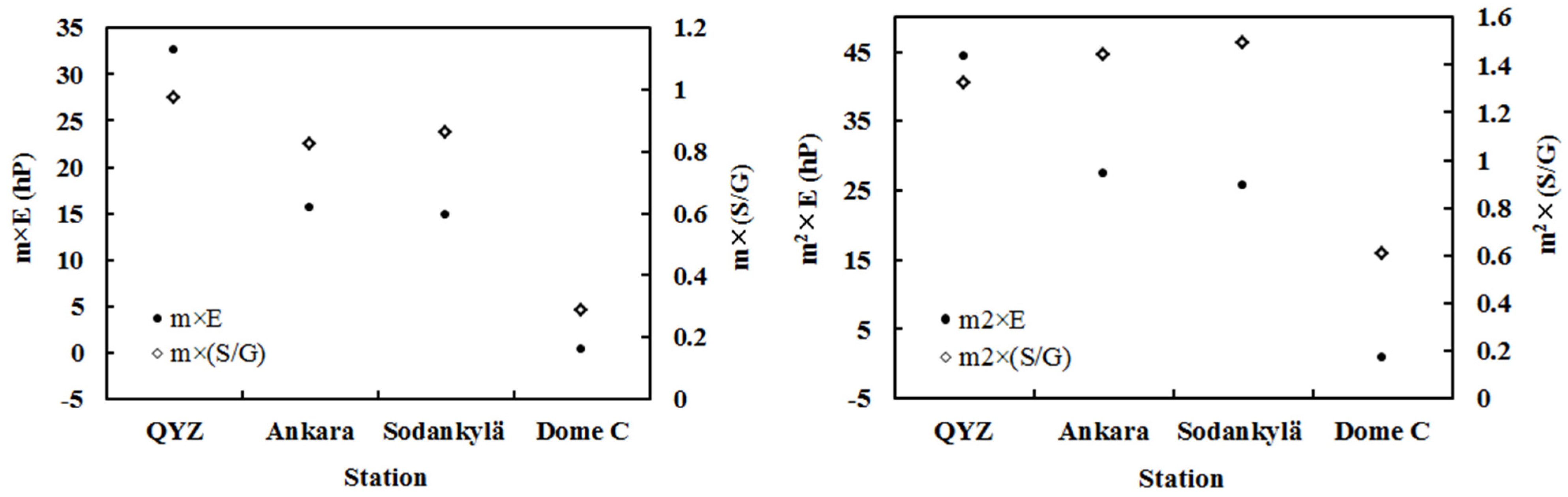
It is necessary to deeply investigate the internal laws for the responses of G to the changes in absorbing and scattering GLPs; thus, the averages of the products of air mass and E, and air mass with S/G, together with the square of air mass and E, and the square of air mass with S/G, when E and S/G increase by 20% and 80%, respectively, were calculated for the four stations (Qianyanzhou, Sodankylä, and Dome C in 2013–2016 and Ankara in 2017–2018). The results are displayed in Table 5 and Figure 14. Combined with the analysis of sensitivity, a similar and better consistency between the change rate of G with E, mE, and m2E was found, meaning that the absorbing GLPs (E) play predominant roles in the change in G, i.e., the responses of G to the change in E were larger at the low-latitude site and decreased stepwise to the lower values at two polar sites. Meanwhile, the best consistency between the change rate of G with m2(S/G) reveals that the multiplicate scattering processes caused by GLPs (i.e., scattering GLPs multiply the realistic optical length) play significant roles. Take the increases in E and S/G by 80% as an example; the correlations between the change rate of G with E, mE, and m2E were −0.91, −0.94, and −0.95, respectively. Similarly, the correlations between the change rate of G with S/G, m(S/G), and m2(S/G) were −0.37, −0.59, and −0.83, respectively. In view of the above results, we should consider many factors driving G change as well as regional climate change, including location, time, season, astronomical factors, atmospheric compositions, and concentrations.
The annual contributions of absorbing loss of G to the total loss in the atmosphere were 79.9% (at S/G < 0.80), 63.3%, 95.5%, and 65.6% for Qianyanzhou, Sodankylä, Dome C, and Ankara, respectively, the corresponding values of scattering loss were 20.1%, 36.7%, 4.5%, and 34.4%, respectively [26,47,48]. Comparing the losses of G in the atmosphere at these four stations, the absorbing loss plays a leading role in the total loss (more than 60%), implying that the absorbing substances were dominant in the GLPs on the Earth.
Based on the above integrated analysis of G and its losses and the sensitivity tests, some multiple interactions and common mechanisms between G and absorbing and scattering GLPs were recognized deeply. On the other hand, the empirical model of global solar radiation was a reliable tool to study solar radiation and its interaction with GLPs.
4.4. Essential Connections of the Atmospheric Components and Their Potential Influences
It is well known and should be emphasized that some basic and significant knowledge, e.g., NOx, SO2, and VOCs, take part in CPRs to produce new GLPs (O3, SOA, black carbon, peroxyacetyl nitrate (PAN), HCHO, etc.), the oxidation products of VOCs (AVOCs and BVOCs) contribute to the formation of condensation nuclei and clouds, and large quantities of substances in the atmosphere have positive or negative radiative forcing [3,33,34,35,40,41,42,43,44,45,54,57,58,59,61,64,65,66,67,68,69,70,71,72,73,74].
In view of the fact that the atmospheric absorbing and scattering substances affect the losses and distributions (GLA, GLS, RLA, and RLS) of G and regional air temperature, more specific studies on all kinds of atmospheric compositions (including GHGs and non-GHGs, or CO2 and non-CO2) and concentrations and their long-term variations are strongly recommended [26,37,75].
To summarize the previous studies about the air temperature increase in the three polar regions (Dome C in Antarctica, Sodankylä in the Arctic, and Qomolangma in the Tibetan Plateau), and a low-latitude site (Qianyanzhou) in the Northern Hemisphere [26,37,47,48], and Ankara in Türkiye (mid-latitude) in this study, it is a basic and effective measure and recommendation to reduce/control the direct emissions of all kinds of GLP emissions and the secondary productions of new GLPs in the atmosphere via CPRs, so as to reduce the increase in atmospheric GLP concentrations along with the increase in the internal energy that kept and accumulated in the atmosphere, and finally, to fulfill the objective of slowing down the regional and global warming.
In the context of climate warming widely experienced in the world, long-term variations in G and atmospheric GLPs and meteorological parameters, along with their multiple interactions, need to be studied thoroughly so as to deeply understand its internal mechanisms and causes and take effective actions to slow down the climate warming.
The sum of the coefficients A1 + A2 + A0 should be equal to the solar constant (4.92 MJ m2, 1367 W m2), and the sum of these coefficients (in Table 1) was 4.55 MJ m2 with a relative error of 7.5%, indicating that timely calibration is necessary. To obtain accurate solar radiation and its effects on climate and climate change, it is suggested to calibrate solar radiation sensors regularly or when they are in need using a calibration method [48,76], which is an effective option that can be easily carried out at the station. Considering atmospheric GLPs (clouds, aerosols, etc.) and sky conditions influence the calibration accuracy, the calibration task is recommended to use the measured solar radiation and meteorological data under clear sky conditions in Ankara province [26,48,76].
4.5. Other Evidence in Air Temperature Increase and Above Mechanisms
The mean annual near-surface air temperature in the northern and southern hemispheres displayed significant increasing trends, with cumulative increases of 0.828 °C and 0.874 °C, respectively. The global land surface air temperature also displayed an increasing trend, with more than 80% of the land surfaces showing a significant increase [77].
Many studies have reported that almost the largest air temperature increasing rate appeared in the winter and the smallest (or lower) in the summer in China (Table 6, Figure 15). This is due to the higher atmospheric components (in GLP phases) produced and present in the atmosphere, which absorb and scatter solar radiation and lead to the atmosphere being warmer in the winter than in the summer. Some studies report that the highest UV and PAR (photosynthetically active radiation) losses in the atmosphere occurred in the winter in North China, which was in good agreement with that of the highest tropospheric NO2 column in the winter [30,31]. In addition, the loss of global solar radiation was higher in the winter and lower in the summer in the Qianyanzhou region [26].
Positive relationships were found between the increasing rate of air temperature and latitude in the winter and summer seasons, more obviously in the winter than in the summer, with a more non-linear relationship than linear (Figure 15). This revealed that (1) the temperature increase varies with latitude (higher in the north and lower in the south). They corresponded to the fact that air temperature increase is the largest in the two polar regions and lower in the low latitude region (Qianyanzhou), which was mainly caused by the differences in per unit atmospheric GLPs, and (2) the non-linear relationship existed between the internal energy of the atmosphere (associated with T) and the total energy absorbed and used by the atmospheric GLPs or net energy of the atmosphere (including short- and long- wave radiation) [37,48,78,79,80,81]. As an example, Equation (1) indicates a non-linear relationship between T (with an internal relation to E) and solar energy (e.g., Gcal); additionally, the sensitivity also revealed a non-linear relation between ΔG and ΔE in Section 3.3. In addition, the air temperature is most sensitive to the change in net radiation than other factors (e.g., S/G, wind speed, and G) [82].
All results in this section provided obvious and additional evidence for the discussed mechanisms in the above sections and this section.

Table 6.
The increasing rate of air temperature (ΔT, °C in 10 years) at some typical sites during the winter and summer seasons in China.
Table 6.
The increasing rate of air temperature (ΔT, °C in 10 years) at some typical sites during the winter and summer seasons in China.
| Site/Region | Latitude (N) | Time Period | ΔT in Winter | ΔT in Summer | Station Number | Reference |
|---|---|---|---|---|---|---|
| Yining | 43.95 | 1952–2015 | 0.47 | 0.31 | Ablat, 2020 [83] | |
| Loess Plateau | 32°–41° | 1960–2013 | 0.41 | 0.15 | 114 | Zhang et al., 2020 [84] |
| Yinchuan | 38.28 | 1960–3019 | 0.60 | 0.34 | Zhang et al., 2012 [85] | |
| Qilianshan | 37°17′–42°48′ | 1965–2018 | 0.36 | 0.31 | Jing et al., 2022 [86] | |
| Jiyang | 37 | 1962–2020 | 0.289 | 0.037 | Wang et al., 2021 [87] | |
| Yutian | 36.51 | 1968–2018 | 0.37 | 0.12 | Aizaitiyuemaier and Yu, 2020 [88] | |
| Xining | 36°37′ (old) 36°44′ (new) | 1954–2016 | 0.44 | 0.38 | Zhu et al., 2021 [89] | |
| Guyuan | 36 | 1961–2021 | 0.537 | 0.304 | Chen et al., 2022 [90] | |
| Lanzhou | 35.52 | 2004–2021 | 0.552 | Yang et al., 2023 [91] | ||
| Wudaoliang | 35.15 | 1961–2019 | 0.42 | 0.30 | Wu et al., 2020 [92] | |
| Sanjiangyuan | 31°39′–36°12′ | 1961–2016 | 0.455 | 0.281 | 23 | Han, 2020 [93] |
| Mianyang | 30°42′–33°03′ | 1954–2016 | 0.186 | 0.112 | Huang, 2021 [94] | |
| Zaduo | 32.53 | 1961–2018 | 0.578 | 0.332 | Han, 2020 [93] | |
| Chengdu | 30.35 | 1961–2019 | 0.268 | 0.126 | Li and Zhang, 2021 [95] | |
| Lasa | 29.67 | 1970–2018 | 0.652 | 0.426 | Lei et al., 2021 [96] | |
| Xinyu | 27.5 | 1959–2019 | 0.27 | 0.043 | Yuan et al., 2022 [97] | |
| Guizhou | 24°30′–29°13′ | 1960–2018 | 0.207 | 0.130 | 34 | Zhao et al., 2021 [98] |
| Tiandong | 23.36 | 1960–2019 | 0.209 | Tan, 2021 [99] |
5. Conclusions
Analyzing solar radiation and meteorological variables measured in Ankara province in Türkiye from 2017 to 2019, an empirical model of global solar radiation was developed and used to compute global solar radiation and its losses in the atmosphere caused by the absorbing and scattering atmospheric substances. This empirical model can reasonably estimate global solar radiation at the ground and be used to study the interactions between solar radiation and the absorbing and scattering GLPs, as well as the causes of air temperature increase. Using this empirical model, the albedos in 2017, 2018, and 2019 were 28.8%, 27.8%, and 28.2%, respectively, at the TOA, and 21.6%, 22.1%, and 21.9%, respectively, at the surface, similar to the corresponding satellite-derived albedos. Calculated and observed global solar radiations decreased by 1.0% per year and 0.1% per year, respectively. The losses of global solar radiation in the atmosphere exhibited clear seasonal variations and were predominated by absorption, indicating that the absorbing substances play leading roles in solar radiation transfer and its attenuation. The sensitivity test showed that global solar radiation was more sensitive to changes in scattering than to changes in absorption, and all responses were negative and non-linear.
Clear positive relationships between v and S/G were found in the Ankara province. The positive and negative relationships between v and S/G were found at four typical regions on the Earth, revealing some interaction mechanisms between the surface structure and the wind. Some common laws were found at four typical sites, e.g., the absorbing substances played dominant roles in global solar radiation transfer and its contribution to loss in the atmosphere. The contributions of absorbing loss in total loss were larger in the low-latitude region and lower in the polar regions, indicating that the absorbing GLPs features were higher in the low-latitude and lower in the polar regions. But the multiple scattering processes played more significant roles in scattering loss than absorbing loss. The realistic optical length and atmospheric substances (concentrations and components) should be considered as a whole. Therefore, we should consider the key geographical and astronomical factors as well as atmospheric factors in solar radiation and its roles in the changes in the atmosphere (e.g., climate warming). To slow down regional and global warming, we should take necessary measures to reduce primary GLP emissions and secondary GLP formation in the atmosphere.
The absorbing and diffusing radiation due to the absorbing and scattering GLPs were calculated at the TOA, in the atmosphere, and at the surface, which are helpful to thoroughly understand solar radiation transfer, energy balance, the interactions in energy—GLPs and energy—atmospheric movements, and T and S/G.
Further research on solar radiation and its roles in the climate and climate change are needed, for example, to carry out studies on long-term variations in more typical regions (including the ocean, if data are available) on Earth. Finally, we will achieve the objectives of thoroughly understanding the whole atmosphere, from phenomena to internal mechanisms and making effective policies toward mitigating climate warming.
Author Contributions
Methodology, investigation, and writing, J.B.; data fusion, X.W. and E.A.; satellite data, X.Z. All authors have read and agreed to the published version of the manuscript.
Funding
This research was supported by the National Natural Science Foundation of China (Grant NO. 42261144751) and Dragon 5 projects (ID 59013).
Data Availability Statement
Not available.
Acknowledgments
Satellite albedo can be accessed via the website https://ceres.larc.nasa.gov/products.php?product=EBAF-Product (accessed on 26 February 2024). Data for this research can be found in a Big Earth Data Platform for Three Poles, http://poles.tpdc.ac.cn/zh-hans/ (accessed on 26 February 2024). The authors thank H.T. Liu and Y.M. Wu from the Institute of Atmospheric Physics, Chinese Academy of Sciences (IAP, CAS) for their help. We thank the Turkish State Meteorology Service for providing the data. The authors give special thanks to anonymous reviewers for their beneficial comments.
Conflicts of Interest
The authors declare no conflicts of interest.
Nomenclature List
| G | global solar radiation (MJ m−2 and W m−2) |
| D | direct normal radiation (MJ m−2 and W m−2) |
| S | diffuse solar radiation (MJ m−2 and W m−2) |
| S/G | scattering factor |
| SZA | solar zenith angle (degree) |
| T | temperature (℃) |
| RH | relative humidity (%) |
| E | water vapor pressure (hPa) |
| Io | solar constant (Wm−2) |
| m | optical air mass (dimensionless) |
| w | precipitable water (mm) |
| △S′ | global solar radiation absorbed by water vapor (W m−2) |
| k | mean absorption coefficient of water vapor (μm) |
| n | sample number |
| R | correlation coefficient |
| R2 | coefficient of determination |
| δ | relative error (%) |
| mean absolute value of relative error (%) | |
| σ | standard deviation |
| GLA | absorbing losses caused by atmospheric GLPs (MJ m−2 and W m−2) |
| GLS | scattering losses (MJ m−2 and W m−2) |
| GL | total losses (MJ m−2 and W m−2) |
| RLA | absorbing losses to the total loss (%) |
| RLS | scattering losses to the total loss (%) |
| v | wind speed (m s−1) |
| p | air pressure (hPa) |
Formulas of δ, , σ, MAD, RMSE, and NMSE
| δ = | |
| σ = | |
| MAD = | |
| RMSE = | |
| NMSE = | |
| n | sample number |
| calculated value | |
| observed value | |
| average of calculated value | |
| average of observed value | |
References
- Guenther, A.; Hewitt, C.N.; Erickson, D.; Fall, R.; Geron, C.; Graedel, T.; Harley, P.; Klinger, L.; Lerdau, M.; McKay, W.A.; et al. A global model of natural volatile organic compound emissions. J. Geophys. Res. 1995, 100, e8873–e8892. [Google Scholar] [CrossRef]
- Sekiyama, T.T.; Kiyotaka, S.; Deushi, M.; Kodera, K.; Lean, J. Stratospheric ozone variation induced by the 11-year solar cycle: Recent 22-year simulation using 3-D chemical transport model with reanalysis data. Geophys. Res. Lett. 2006, 33, L17812. [Google Scholar] [CrossRef]
- Bai, J.H.; Leeuw G de van der, A.R.; Smedt, I.; De Theys, N.; Van Roozendael, M.; Sogacheva, L.; Chai, W.H. Variations and photochemical transformations of atmospheric constituents in North China. Atmos. Environ. 2018, 189, 213–226. [Google Scholar] [CrossRef]
- Madronich, S.; Flocke, S. The Role of Solar Radiation in Atmospheric Chemistry. In Environmental Photochemistry, Vol. 2/2L of the Handbook of Environmental Chemistry; Boule, P., Ed.; Springer: Berlin/Heidelberg, Germany, 1999; pp. 1–26. [Google Scholar]
- Solanki, S.K. Solar variability and climate change is there a link. Harold Jeffreys Lect. 2002, 43, 5. [Google Scholar] [CrossRef]
- Elminir, H.K. Relative influence of weather conditions and air pollutants on solar radiation—Part 2: Modification of solar radiation over urban and rural sites. Meteorol. Atmos. Phys. 2007, 96, 257–264. [Google Scholar] [CrossRef]
- Trenberth, K.E.; Fasullo, J.T.; Kiehl, J. Earth’s global energy budget. Bull. Am. Meteorol. Soc. 2009, 90, 311–323. [Google Scholar] [CrossRef]
- Lean, J.; Rind, D. Climate forcing by changing solar radiation. J. Clim. 2010, 11, 3069–3094. [Google Scholar] [CrossRef]
- Andreae, M.O.; Ramanathan, V. Climate’s Dark Forcings. Sciences 2013, 340, 280–281. [Google Scholar] [CrossRef]
- Rosenfeld, D.; Sherwood, S.; Wood, R.; Donner, L. Climate Effects of Aerosol-Cloud Interactions. Sciences 2014, 343, 379–380. [Google Scholar] [CrossRef]
- Calabrò, E.; Magazù, S. Correlation between Increases of the Annual Global Solar Radiation and the Ground Albedo Solar Radiation due to Desertification—A Possible Factor Contributing to Climatic Change. Climate 2016, 4, 64. [Google Scholar] [CrossRef]
- Glower, J.; McGulloch, J.S.G. The empirical relation between solar radiation and hours of sunshine. Quart. JR. Met. Soc. 1958, 84, 172–175. [Google Scholar]
- Atwater, M.A.; Ball, J.T. A numerical solar radiation model based on standard meteorological observations. Sol. Energy 1978, 21, 163–170, Erratum in Sol. Energy 1978, 123, 275. [Google Scholar] [CrossRef]
- Bird, R.E. A simple solar spectral model for direct-normal and diffuse horizontal irradiance. Sol. Energy 1984, 32, 461–471. [Google Scholar] [CrossRef]
- Gueymard, C.A. Critical analysis and performance assessment of clear sky solar irradiance models using theoretical and measured data. Sol. Energy 1993, 51, 121–138. [Google Scholar] [CrossRef]
- Gueymard, C.A. Clear-Sky Radiation Models and Aerosol Effects. Sol. Resour. Mapp. 2019, 137–182. [Google Scholar] [CrossRef]
- Myers, D.R. Solar radiation modeling and measurements for renewable energy applications data and model quality. Energy 2005, 30, 1517–1531. [Google Scholar] [CrossRef]
- Badescu, V.; Gueymard, C.A.; Cheval, S.; Oprea, C.; Baciu, M.; Dumitrescu, A.; Iacobescu, F.; Milos, I.; Rada, C. Accuracy analysis for fifty-four clear-sky solar radiation models using routine hourly global irradiance measurements in Romania. Renew. Energy 2013, 55, 85–103. [Google Scholar] [CrossRef]
- Besharat, F.; Dehghan, A.A.; Faghih, A. Empirical models for estimating global solar radiation: A review and case study. Renew. Sust. Energ. Rev. 2013, 21, 798–821. [Google Scholar] [CrossRef]
- Bayrakc, H.C.; Demircan, C.; Keceba, A. The development of empirical models for estimating global solar radiation on horizontal surface: A case study. Renew. Sust. Energ. Rev. 2018, 81, 2771–2782. [Google Scholar] [CrossRef]
- Antonanzas-Torres, F.; Urraca, R.; Polo, J.; Perpinan-Lamigueiro, O.; Escobar, R. Clear sky solar irradiance models: A review of seventy models. Renew. Sust. Energ. Rev. 2019, 107, 374–387. [Google Scholar] [CrossRef]
- Kosmopoulos, P.G.; Kazadzis, S.; Lagouvardos, K.; Kotroni, V.; Bais, A. Solar energy prediction and verification using operational model forecasts and ground-based solar measurements. Energy 2015, 93, 1918–1930. [Google Scholar] [CrossRef]
- Zang, H.X.; Jiang, X.; Cheng, L.L.; Zhang, F.C.; Wei, Z.N.; Sun, G.Q. Combined empirical and machine learning modeling method for estimation of daily global solar radiation for general meteorological observation stations. Renew. Energy 2022, 195, 795–808. [Google Scholar] [CrossRef]
- Aras, H.; Balli, O.; Hepbasli, A. Estimating the horizontal diffuse solar radiation over the Central Anatolia Region of Turkey. Energy Convers. Manag. 2006, 47, 2240–2249. [Google Scholar] [CrossRef]
- Ülgen, K.; Hepbasli, A. Diffuse solar radiation estimation models for Turkey’s big cities. Energy Convers. Manag. 2009, 50, 149–156. [Google Scholar] [CrossRef]
- Bai, J.; Zong, X. Global Solar Radiation Transfer and its Loss in the Atmosphere. Appl. Sci. 2021, 11, 2651. [Google Scholar] [CrossRef]
- Salmon, A.; Marzo, A.; Polo, J.; Ballestrín, J.; Carra, E.; Alonso-Montesinos, J. World map of low-layer atmospheric extinction values for solar power tower plants projects. Renew. Energy 2022, 201, 876–888. [Google Scholar] [CrossRef]
- Bilbao, J.S.; Vill’an, D.M.; de M Castrillo, A. Analysis and cloudiness influence on UV total irradiation. J. Climatol. 2011, 31, 451–460. [Google Scholar]
- Bai, J.H. Analysis of ultraviolet radiation in clear skies in Beijing and its affecting factors. Atmos. Environ. 2011, 45, 6930–6937. [Google Scholar] [CrossRef]
- Bai, J.H. Photosynthetically active radiation loss in the atmosphere in North China. Atmos. Pollut. Res. 2013, 4, 411–419. [Google Scholar] [CrossRef]
- Bai, J.H. UV extinction in the atmosphere and its spatial variation in North China. Atmos. Environ. 2017, 154, 318–330. [Google Scholar] [CrossRef]
- Du, J.; Huang, L.; Min, Q.; Zhu, L. The Influence of Water Vapor Absorption in the 290–350 nm Region on Solar Radiance: Laboratory Studies and Model Simulation. Geophys. Res. Lett. 2013, 40, 4788–4792. [Google Scholar] [CrossRef]
- Li, S.P.; Matthews, J.; Sinha, A. Atmospheric hydroxyl radical production from electronically excited NO2 and H2O. Science 2008, 319, 1657–1660. [Google Scholar] [CrossRef]
- Matthews, J.; Sinha, A.; Francisco, J.S. The importance of weak absorption features in promoting tropospheric radical production. Proc. Natl. Acad. Sci. USA 2005, 102, 7449–7452. [Google Scholar] [CrossRef]
- Wilson, E.M.; Wenger, J.C.; Venables, D.S. Upper limits for absorption by water vapor in the near-UV. J. Quantitat. Spectrosc. Radiat. Transf. 2016, 170, 194–199. [Google Scholar] [CrossRef]
- Kondratyev, K. Solar Energy; Science Press: Beijing, China, 1962; pp. 123–132. [Google Scholar]
- Bai, J.H.; Zong, X.M.; Ma, Y.M.; Wang, B.B.; Zhao, C.F.; Yang, Y.K.; Guang, J.; Cong, Z.Y.; Li, K.L.; Song, T. Long-term variations in global solar radiation and its interaction with atmospheric substances at Qomolangma. Int. J. Environ. Res. Public Health 2022, 19, 8906. [Google Scholar] [CrossRef]
- Tariq, S.; Zeydan, Ö.; Nawaz, H.; Mehmood, U.; ul-Haq, Z. Impact of land use/land cover (LULC) changes on latent/sensible heat flux and precipitation over Türkiye. Theor. Appl. Climatol. 2023, 153, 1237–1256. [Google Scholar] [CrossRef]
- Yang, S.; Wang, X.L.; Wild, M. Causes of Dimming and Brightening in China Inferred from Homogenized Daily Clear-Sky and All-Sky in situ Surface Solar Radiation Records (1958–2016). J. Clim. 2019, 32, 5901–5913. [Google Scholar] [CrossRef]
- Bai, J.H.; Guenther, A.; Turnipseed, A.; Duhl, T.; Greenberg, J. Seasonal and interannual variations in whole-ecosystem BVOC emissions from a subtropical plantation in China. Atmos. Environ. 2017, 161, 176–190. [Google Scholar] [CrossRef]
- Carlton, A.G.; Wiedinmyer, C.; Kroll, J.H. A review of secondary organic aerosol (SOA) formation from isoprene. Atmos. Chem. Phys. 2009, 9, 4987–5005. [Google Scholar] [CrossRef]
- Horowitz, A.; Meller, R.; Moortgat, G.K. The UV-VIS absorption cross sections of the a- dicarbonyl compounds: Pyruvic acid, biacetyl and glyoxal. J. Photochem. Photobiol. A Chem. 2001, 146, 19–27. [Google Scholar] [CrossRef]
- Hansel, A.K.; Ehrenhauser, F.S.; Richards-Henderson, N.K.; Anastasio, C.; Valsaraj, K.T. Aqueous-phase oxidation of green leaf volatiles by hydroxyl radical as a source of SOA: Product identification from methyl jasmonate and methyl salicylate oxidation. Atmos. Environ. 2015, 102, 43–51. [Google Scholar] [CrossRef]
- Jacobson, M. Isolating nitrated and aromatic aerosols and nitrated aromatic gases as sources of ultraviolet light absorption. J. Geophys. Res. 1999, 104, 3527–3542. [Google Scholar] [CrossRef]
- Jonsson, Å.M.; Hallquist, M.; Ljungström, E. Influence of OH Scavenger on the Water Effect on Secondary Organic Aerosol Formation from Ozonolysis of Limonene, Δ3-Carene, and α-Pinene. Environ. Sci. Technol. 2008, 42, 5938–5944. [Google Scholar] [CrossRef]
- Zeydan, Ö.; Tariq, S.; Qayyum, F.; Mehmood, U.; Ul-Haq, Z. Investigating the long-term trends in aerosol optical depth and its association with meteorological parameters and enhanced vegetation index over Turkey. Environ. Sci. Pollut. Res. 2022, 30, 20337–20356. [Google Scholar] [CrossRef]
- Bai, J.H.; Zong, X.M.; Lanconelli, C.; Lupi, A.; Driemel, A.; Vitale, V.; Li, K.L.; Song, T. Long-Term Variations of Global Solar Radiation and Its Potential Effects at Dome C (Antarctica). Int. J. Environ. Res. Public Health 2022, 19, 3084. [Google Scholar] [CrossRef]
- Bai, J.; Heikkilä, A.; Zong, X. Long-Term Variations of Global Solar Radiation and Atmospheric Constituents at Sodankylä in the Arctic. Atmosphere 2021, 12, 749. [Google Scholar] [CrossRef]
- Dickinson, R.E. Land surface processes and climate surface albedos and energy balance. Adv. Geophys. 1983, 25, 305–353. [Google Scholar]
- Psiloglou, B.E.; Kambezidis, H.D. Estimation of the ground albedo for the Athens area, Greece. J. Atmos. Solar-Terr. Phys. 2009, 71, 943–954. [Google Scholar] [CrossRef]
- Loeb, N.G.; Doelling, D.R.; Wang, H.; Su, W.; Nguyen, C.; Corbett, J.G.; Liang, L.; Mitrescu, C.; Rose, F.G.; Kato, S. Clouds and the Earth’s Radiant Energy System (CERES) Energy Balanced and Filled (EBAF) Top-of-Atmosphere (TOA) Edition 4.0 Data Product. J. Clim. 2018, 31, 895–918. [Google Scholar] [CrossRef]
- Kato, S.; Rose, F.G.; Rutan, D.A.; Thorsen, T.J.; Loeb, N.G.; Doelling, D.R.; Huang, X.; Smith, W.L.; Su, W.; Ham, S.H. Surface Irradiances of Edition 4.0 Clouds and the Earth’s Radiant Energy System (CERES) Energy Balanced and Filled (EBAF) Data Product. J. Clim. 2018, 31, 4501–4527. [Google Scholar] [CrossRef]
- Sun, Y.J.; Wang, Z.H.; Qin, Q.M.; Han, G.H.; Ren, H.Z.; Huang, J.F. Retrieval of surface albedo based on GF-4geostationary satellite image data. J. Remote Sens. 2018, 22, 220–233. [Google Scholar]
- Chen, C.; Park, T.; Wang, X.; Piao, S.; Xu, B.; Chaturvedi, R.K.; Fuchs, R.; Brovkin, V.; Ciais, P.; Fensholt, R.; et al. China and India lead in greening of the world through land-use management. Nat. Sustain. 2019, 2, 122–129. [Google Scholar] [CrossRef]
- Claeys, M.; Graham, B.; Vas, G.; Wang, W.; Vermeylen, R.; Pashynska, V.; Cafmeyer, J.; Guyon, P.; Andreae, M.O.; Artaxo, P.; et al. Formation of secondary organic aerosols through photooxidation of isoprene. Science 2004, 303, 1173–1176. [Google Scholar] [CrossRef]
- Shen, Z.B.; Wang, Y.Q.; Wang, W.H.; Wu, J.Z. The attenuation of solar radiation in the polluted urban atmosphere. Plateau Meteoro. 1982, 1, 74–83. [Google Scholar]
- Sweerts, B.; Pfenninger, S.; Yang, S.; Folini, D.; van der Zwaan, B.; Wild, M. Estimation of losses in solar energy production from air pollution in China since 1960 using surface radiation data. Nat. Energy 2019, 4, 657–663. [Google Scholar] [CrossRef]
- von Schuckmann, K.; Palmer, M.D.; Trenberth, K.E.; Cazenave, A.; Chambers, D.; Champollion, N.; Hansen, J.; Josey, S.A.; Loeb, N.; Mathieu, P.-P.; et al. An imperative to monitor Earth’s energy imbalance. Nat. Clim. Change 2016, 6, 138–144. [Google Scholar] [CrossRef]
- Sun, Y.; Jiang, Q.; Xu, Y.; Ma, Y.; Zhang, Y.; Liu, X.; Li, W.; Wang, F.; Li, J.; Wang, P.; et al. Aerosol characterization over the North China Plain: Haze life cycle and biomass burning impacts in summer. J. Geophys. Res. 2016, 121, 2508–2521. [Google Scholar] [CrossRef]
- Valero, F.P.J.; Pope, S.K.; Bush, B.C.; Nguyen, Q.; Marsden, D.; Cess, R.D.; Simpson-Leitner, A.S.; Bucholtz, A.; Udelhofen, P.M. Absorption of solar radiation by the clear and cloudy atmosphere during the Atmospheric Radiation Measurement Enhanced Shortwave Experiments (ARESE) I and II: Observations and models. J. Geophys. Res. Atmos. 2003, 108, 4016. [Google Scholar] [CrossRef]
- Xu, W.; Xie, C.; Karnezi, E.; Zhang, Q.; Wang, J.; Pandis, S.N.; Sun, Y. Summertime aerosol volatility measurements in Beijing, China. Atmos. Chem. Phys. 2019, 19, 10205–10216. [Google Scholar] [CrossRef]
- Zavalishin, N.N. Reasons for Modern Warming: Hypotheses and Facts. J. Atmos. Sci. Res. 2022, 5, 11–17. [Google Scholar]
- Kambezidis, H.D. The Solar Radiation Climate of Greece. Climate 2021, 9, 183. [Google Scholar] [CrossRef]
- Atkinson, R. Atmospheric chemistry of VOCs and NOx. Atmos. Environ. 2000, 34, 2063–2101. [Google Scholar] [CrossRef]
- Chu, B.; Kerminen, V.M.; Bianchi, F.; Yan, C.; Petäjä, T.; Kulmala, M. Atmospheric new particle formation in China. Atmos. Chem. Phys. 2019, 19, 115–138. [Google Scholar] [CrossRef]
- Dunne, E.M.; Gordon, H.; Kürten, A.; Almeida, J.; Duplissy, J.; Williamson, C.; Ortega, I.K.; Pringle, K.J.; Adamov, A.; Baltensperger, U.; et al. Global atmospheric particle formation from CERN CLOUD. Science 2016, 354, 1119–1124. [Google Scholar] [CrossRef]
- Ehn, M.; Thornton, J.A.; Kleist, E.; Sipilä, M.; Junninen, H.; Pullinen, I.; Springer, M.; Rubach, F.; Tillmann, R.; Lee, B.; et al. A large source of low-volatility secondary organic aerosol. Nature 2014, 506, 476–479. [Google Scholar] [CrossRef]
- Hoffer, A.; Gelencs, A.; Guyon, P.; Kiss, G.; Schmid, O.; Frank, G.P.; Artaxo, P.; Andreae, M.O. Optical properties of humic-like substances (HULIS) in biomass burning aerosols. Atmos. Chem. Phys. 2006, 6, 3563–3570. [Google Scholar] [CrossRef]
- Kiendler-Scharr, A.; Wildt, J.; Dal Maso, M.; Hohaus, T.; Kleist, E.; Mentel, T.F.; Tillmann, R.; Uerlings, R.; Schurr, U.; Wahner, A. New particle formation in forests inhibited by isoprene emissions. Nature 2009, 461, 381–384. [Google Scholar] [CrossRef]
- Kirchstetter, T.W.; Novakov, T.; Hobbs, P.V. Evidence that the spectral dependence of light absorption by aerosols is affected by organic carbon. J. Geophys. Res. 2004, 109, D21208. [Google Scholar] [CrossRef]
- McVay, R.C.; Zhang, X.; Aumont, B.; Valorso, R.; Camredon, M.; La, Y.Y.S.; Wennberg, P.O.; Seinfeld, J.H. SOA formation from the photooxidation of α-pinene: Systematic exploration of the simulation of chamber data. Atmos. Chem. Phys. 2016, 16, 2785–2802. [Google Scholar] [CrossRef]
- Mielonen, T.; Hienola, A.; Kühn, T.; Merikanto, J.; Lipponen, A.; Bergman, T.; Korhonen, H.; Kolmonen, P.; Sogacheva, L.; Ghent, D.; et al. Summertime Aerosol Radiative Effects and Their Dependence on Temperature over the Southeastern USA. Atmosphere 2018, 9, 180. [Google Scholar] [CrossRef]
- Penuelas, J.; Llusia, J. BVOCs: Plant defense against climate warming? Trends Plant Sci. 2003, 8, 105–109. [Google Scholar] [CrossRef]
- Guyon, P.; Graham, B.; Roberts, G.C.; Mayol-Bracero, O.L.; Maenhaut, W.; Artaxo, P.; Andreae, M.O. Sources of optically active aerosol particles over the Amazon forest. Atmos. Environ. 2004, 38, 1039–1051. [Google Scholar] [CrossRef]
- Fuglestvedt, J.; Lund, M.T.; Kallbekken, S.; Samset, B.H.; Lee, D.S. A “greenhouse gas balance” for aviation in line with the Paris Agreement. WIREs Clim. Change 2023, 14, e839. [Google Scholar] [CrossRef]
- Bai, J.H. A calibration method of solar radiometers. Atmos. Pollut. Res. 2019, 10, 1365–1373. [Google Scholar] [CrossRef]
- Shen, B.B.; Song, S.F.; Zhang, L.J.; Wang, Z.Q.; Ren, C.; Li, Y.S. Changes in global air temperature from 1981 to 2019, 2021. Acta Geogr. Sinaca 2021, 76, 2660–2672. [Google Scholar]
- Vaughan, D.G.; Marshall, G.J.; Connolley, W.M.; King, J.C.; Mulvaney, R. Climate Change: Devil in the Detail. Science 2001, 293, 1777–1779. [Google Scholar] [CrossRef]
- Vaughan, D.; Marshall, G.J.; Connolley, W.M.; Parkinson, C.; Mulvaney, R.; Hodgson, D.A.; King, J.C.; Pudsey, C.J.; Turner, J. Recent Rapid Regional ClimateWarming on the Antarctic Peninsula. Clim. Chang. 2003, 60, 243–274. [Google Scholar] [CrossRef]
- Vaughan, D.G. British Antarctic Survey; Natural Environment Research Council, Madingley Road, Cambridge CB3 0ET, United Kingdom. 2007. Available online: http://www.homepages.ed.ac.uk/shs/Climatechange/Data%20sources/antarctic_peninsula.php.htm (accessed on 17 January 2022).
- Turner, J.; Colwell, S.R.; Marshall, G.J.; Lachlan-Cope, T.A.; Carleton, A.M.; Jones, P.D.; Lagun, V.; Reid, P.A.; Iagovkina, S.V. Antarctic climate change during the last 50 years. Int. J. Climatol. 2005, 25, 279–294. [Google Scholar] [CrossRef]
- Bai, J.H.; Wang, G.C. Correlation between temperature and surface radiation budget: Analysis of observational data from Yucheng and Luancheng stations. Meteorol. Mon. 2013, 39, 1437–1444. [Google Scholar]
- Ablat, R. Analysis on the characteristics of temperature and precipitation changes in Yining, Xinjiang from 1952 to 2015. Shaanxi Water Resour. 2020, 12, 20–25. [Google Scholar]
- Zhang, Y.Z.; Zhang, B.; Liu, Y.Y.; Zhang, D.Y. Response of variability of temperature in the Loess Plateau to the Hiatus in the process of global warming in the period from 1960 and 2013. Res. Soil Water Conserv. 2020, 27, 213–219. [Google Scholar]
- Zhang, Y.Q.; Xiao, G.J.; Chen, M.J. Analysis on the characteristics of temperature change in Yinchuan in recent 60 years. J. Chengdu Univ. Inf. Technol. 2012, 36, 680–686. [Google Scholar]
- Jing, W.M.; Ren, X.F.; Zhao, W.J. Spatio-temporal Pattern variations of temperature and precipitation in northern parts of the Qilian Mountains and the nearby regions from 1965 to 2018. Plateau Meteorol. 2022, 41, 876–886. [Google Scholar] [CrossRef]
- Wang, H.; Wang, G.H.; Lu, Q. Analysis of temperature variation characteristics in jiyang, shandong province in recent 59 years. J. Agric. Catastropholgy 2021, 11, 53–55. [Google Scholar]
- Aizaitiyuemaier, D.; Yu, Y.H. Change of Mean Temperature and extreme temperature in yutian in the past 50 years. J. Henan Sci. Technol. 2020, 702, 137–141. [Google Scholar]
- Zhu, B.W.; Zhang, L.Z.; Xie, Q.Y.; Zhang, C. Characteristics of temperature change in Xining city from 1954 to 2016. Meteorol. Hudrological Mar. Instrum. 2021, 4, 117–120. [Google Scholar]
- Chen, W.; Yang, W.H.; Jing, B. Characteristics of climate change and its effects on apricot growth in Yuanzhou District, Guyuan in recent 61 years. Agric. Sci.-Technol. Inf. 2022, 22, 51–54. [Google Scholar]
- Yang, T.; Liang, Y.P.; Tao, Y.Y. Analysis on the characteristics of temperature change in Lanzhou city in recent 18 years. J. Lanzhou Petrochem. Polytech. 2023, 23, 24–28. [Google Scholar]
- Wu, S.G.; Han, T.F.; Zhang, D.Q.; Li, J.F. Climate change analysis of wudaolıang area 1961–2019. Qinghai Pratacult. 2020, 29, 48–58. [Google Scholar]
- Han, F.X. Variation characteristics of temperature in Sanjiangyuan area in 1961–2016. Qinghai Prataculture 2020, 29, 38–44. [Google Scholar]
- Huang, X. Analysis of characteristics of climate change in mianyang city in recent 60 years. Henan Sci. Technol. 2021, 758, 104–109. [Google Scholar]
- Li, Q.S.; Zhang, J.H. Analysis of temperature variation characteristics in shuangliu district from 1961 to 2019. J. Agric. Catastropholgy 2021, 11, 112–114. [Google Scholar]
- Lei, Y.; Wang, H.B.; Lu, T.S.; Liu, L.L.; Fu, W.X.; Wei, D. Characteristics of air temperature variation in lhasa city over the past 49 years. Earth Environ. 2021, 49, 492–503. [Google Scholar]
- Yuan, C.; Li, H.H.; Ma, Z.Y.; Li, X.J.; Xiao, Y. Analysis of temperature Cchange Ttrend in Xinyu City in recent 60 Years. Jiangxi Sci. 2022, 40, 498–501. [Google Scholar] [CrossRef]
- Zhao, Z.L.; Luo, Y.; Yang, S.T.; Yu, J.L.; Liu, Y.; Shi, C.M.; Xue, X. Characteristics of temperature spatiotemporal variations in Guizhou Plateau from 1960 to 2018 based on homogenized sequence. J. Water Resour. Water Eng. 2021, 32, 81–89. [Google Scholar]
- Tan, X.T. Analysis of temperature variation characteristics in tiandong county in recent 60 years. J. Agric. Catastropholgy 2021, 11, 77–80. [Google Scholar]
Figure 1.
Flowchart for the development of an empirical model of global solar radiation (G), the calculation processes of A1, A2, A0, etc.
Figure 1.
Flowchart for the development of an empirical model of global solar radiation (G), the calculation processes of A1, A2, A0, etc.
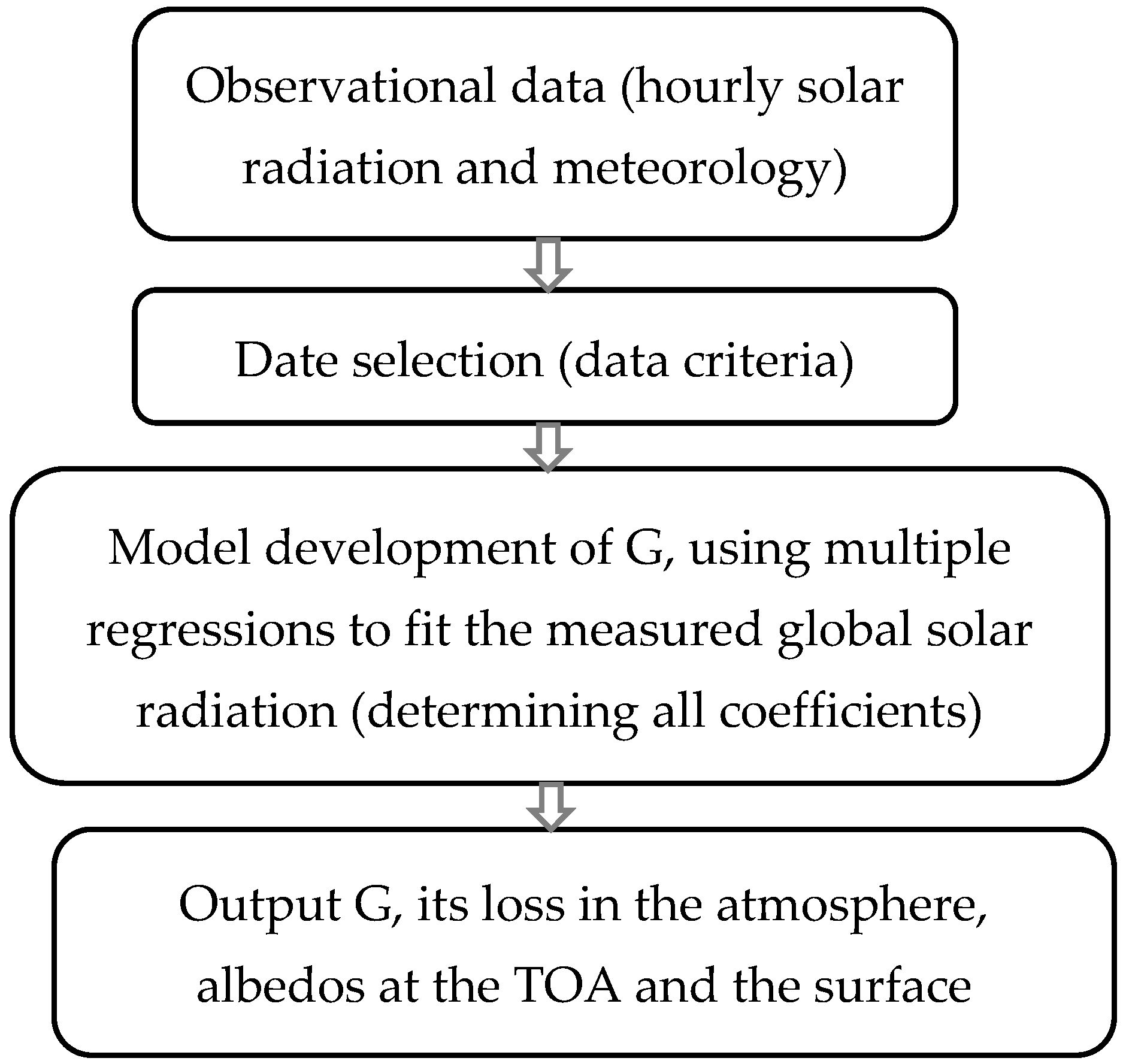
Figure 2.
(a) The observed and calculated monthly averages of hourly global solar exposure (i.e., solar irradiation, Gobs, and Gcal) and relative biases (δ) in all sky conditions in Ankara province. The error bars show the standard deviations of the observed values (up). (b,c) Scatter plots of calculated versus observed hourly (bottom left, n = 6160) and monthly (bottom right, n = 24) global solar exposure under all skies in Ankara province, respectively.

Figure 3.
Monthly averages of observed and calculated hourly global solar exposure (Gobs and Gcal) and S/G under all sky conditions in 2017–2019. The error bars show the standard deviations of the observed values.
Figure 3.
Monthly averages of observed and calculated hourly global solar exposure (Gobs and Gcal) and S/G under all sky conditions in 2017–2019. The error bars show the standard deviations of the observed values.
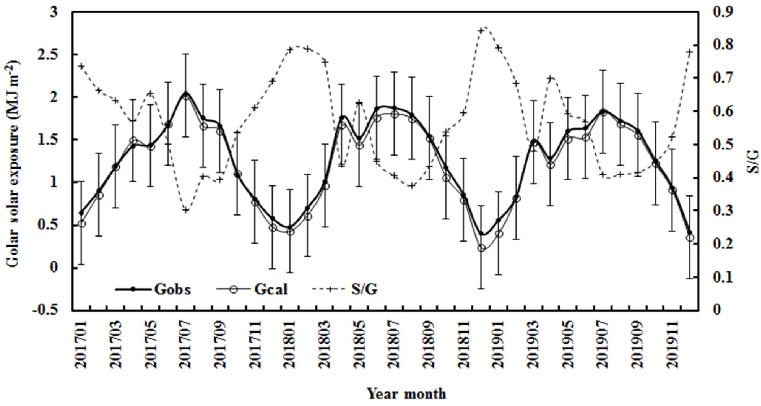
Figure 4.
Monthly mean losses (left) of the global solar radiation and their influencing factors (E, S/G, right) from 1 January 2017 to December 2019.
Figure 4.
Monthly mean losses (left) of the global solar radiation and their influencing factors (E, S/G, right) from 1 January 2017 to December 2019.

Figure 5.
Seasonal mean losses of global solar radiation (GLA and GLS) and their total loss (GL), and water vapor pressure (E) and S/G.
Figure 5.
Seasonal mean losses of global solar radiation (GLA and GLS) and their total loss (GL), and water vapor pressure (E) and S/G.
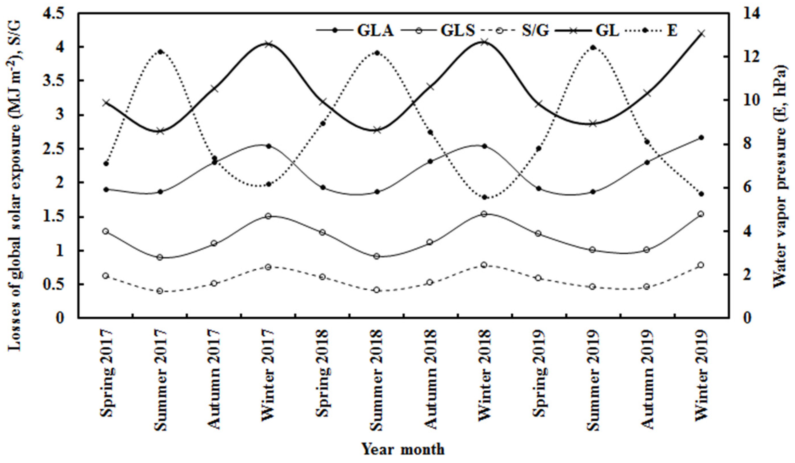
Figure 6.
Changing rates of global solar radiation (%) caused by the changes in one factor (%), while another factor remained at its original level.
Figure 6.
Changing rates of global solar radiation (%) caused by the changes in one factor (%), while another factor remained at its original level.

Figure 7.
Averages of hourly wind speed and atmospheric substance (S/G) for the x axis using the S/G interval at 0.05 ranging from 0.0 to 1.00 (left) and their scatter plot (right) from January 2017 to December 2019.
Figure 7.
Averages of hourly wind speed and atmospheric substance (S/G) for the x axis using the S/G interval at 0.05 ranging from 0.0 to 1.00 (left) and their scatter plot (right) from January 2017 to December 2019.

Figure 8.
Scatter plot of (a, left) wind speed versus air pressure and (b, middle) air pressure versus S/G, and v and S/G (c, right) at different S/G intervals of 0.05 under all sky conditions in Ankara province in January 2017–December 2019.
Figure 8.
Scatter plot of (a, left) wind speed versus air pressure and (b, middle) air pressure versus S/G, and v and S/G (c, right) at different S/G intervals of 0.05 under all sky conditions in Ankara province in January 2017–December 2019.
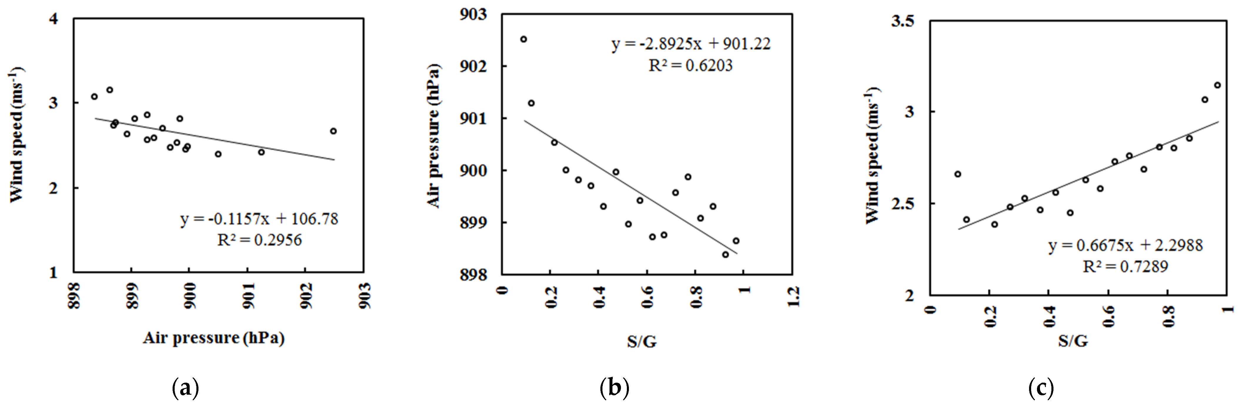
Figure 9.
Annual mean albedos from 2017 to 2019, calculated (cal) and satellite-retrieved (sat) at the TOA and the surface under all sky conditions.
Figure 9.
Annual mean albedos from 2017 to 2019, calculated (cal) and satellite-retrieved (sat) at the TOA and the surface under all sky conditions.
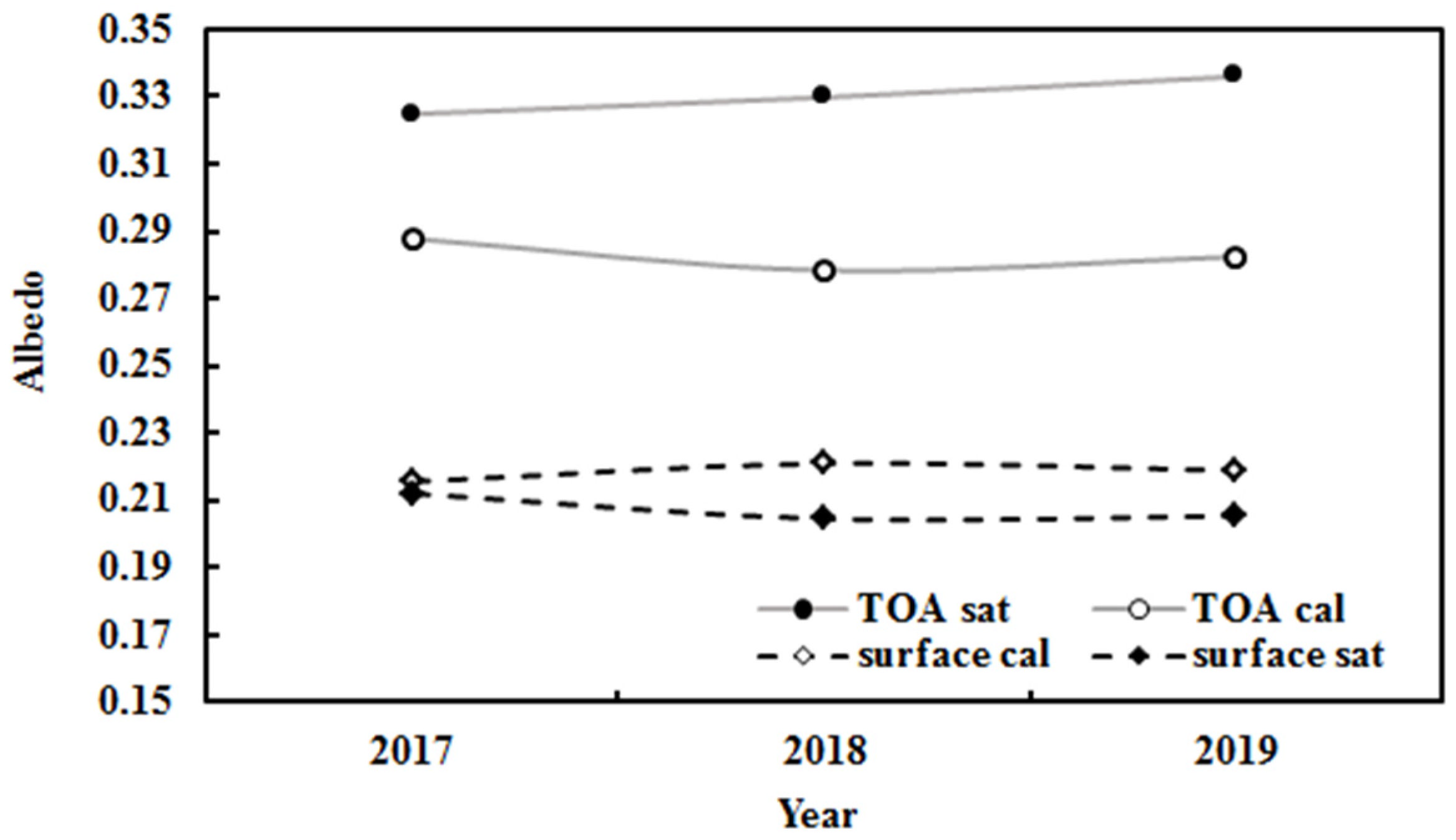
Figure 10.
Ratio of solar absorbing loss to S/G and then to air temperature (T) at different S/G intervals in Ankara province in 2017–2019.
Figure 10.
Ratio of solar absorbing loss to S/G and then to air temperature (T) at different S/G intervals in Ankara province in 2017–2019.
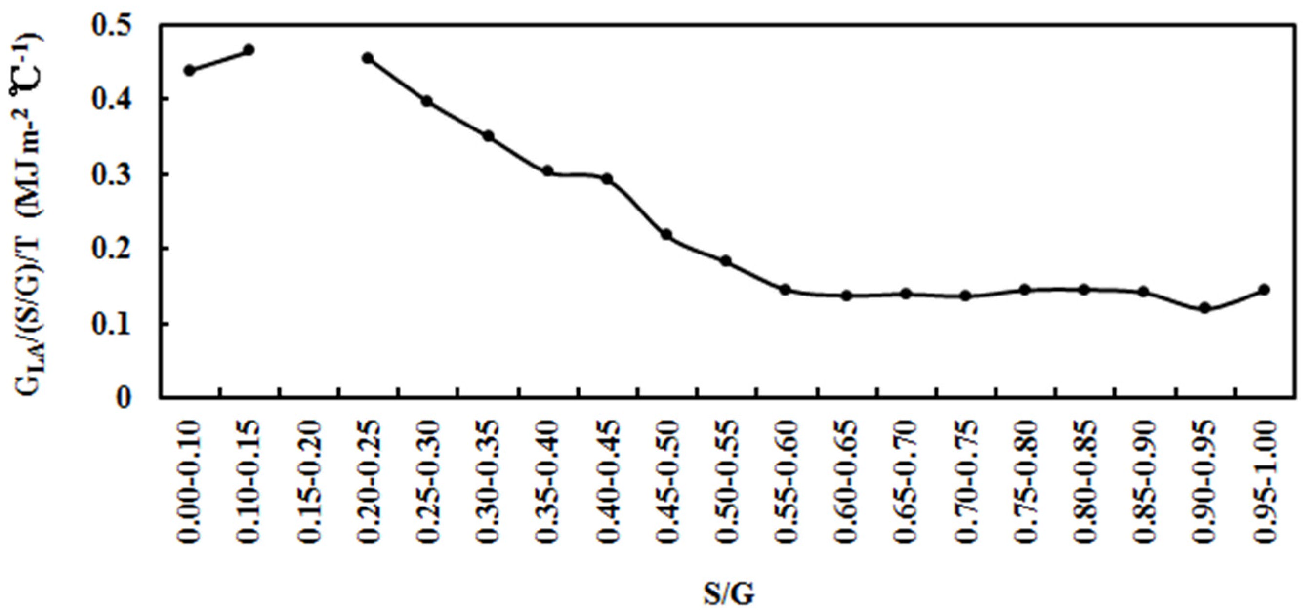
Figure 11.
Scatter plot of the annual averages of air temperature verse S/G under all sky conditions in Ankara province in 2017–2019.
Figure 11.
Scatter plot of the annual averages of air temperature verse S/G under all sky conditions in Ankara province in 2017–2019.
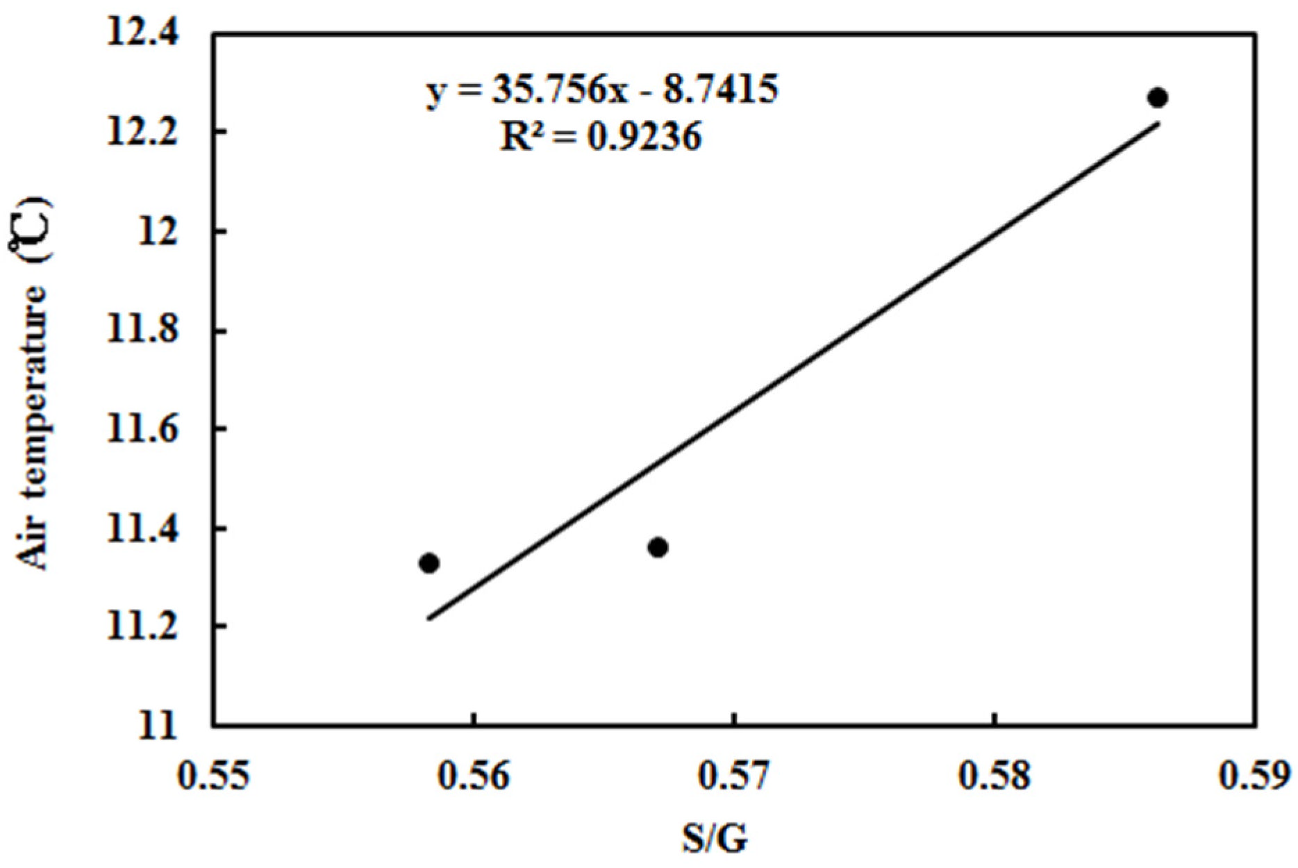
Figure 12.
Scatter plot of the annual averages of air temperature and S/G under all sky conditions at four sites (Sodankylä, Dome C, Ankara, and Qianyanzhou, left), and the calculated air temperature using Equation (6) between T and S/G determined at these four stations (right).
Figure 12.
Scatter plot of the annual averages of air temperature and S/G under all sky conditions at four sites (Sodankylä, Dome C, Ankara, and Qianyanzhou, left), and the calculated air temperature using Equation (6) between T and S/G determined at these four stations (right).
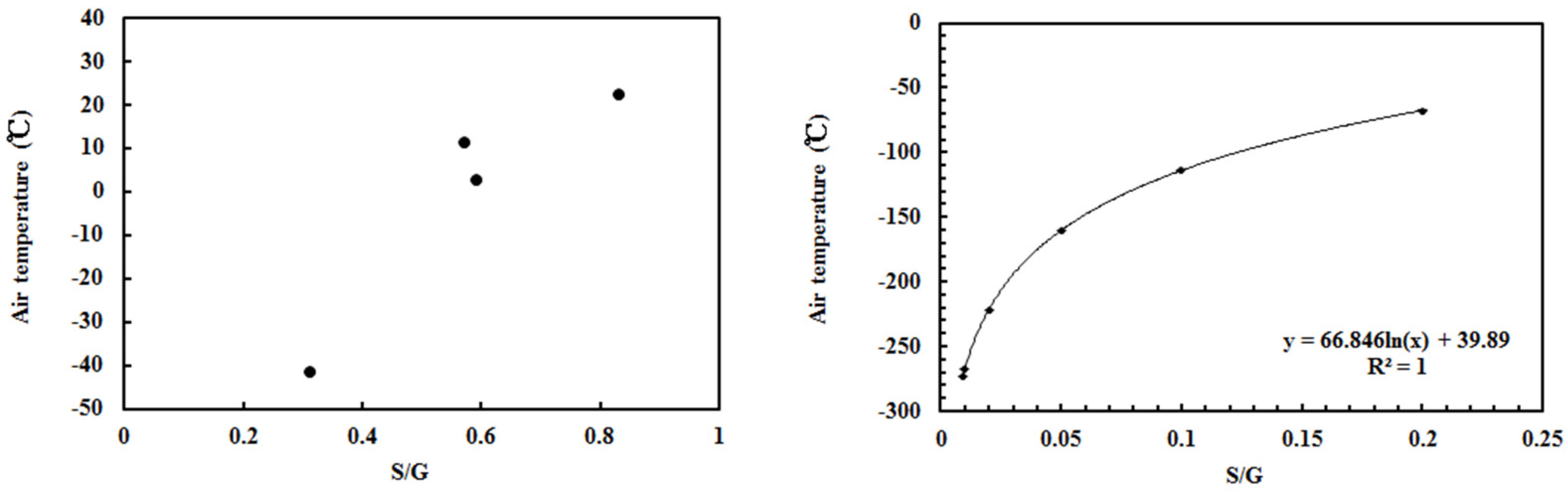
Figure 13.
Changing rates of G (%) caused by the changes in one factor (+20%, +80%), while another factor remained at its original level at four typical sites.
Figure 13.
Changing rates of G (%) caused by the changes in one factor (+20%, +80%), while another factor remained at its original level at four typical sites.
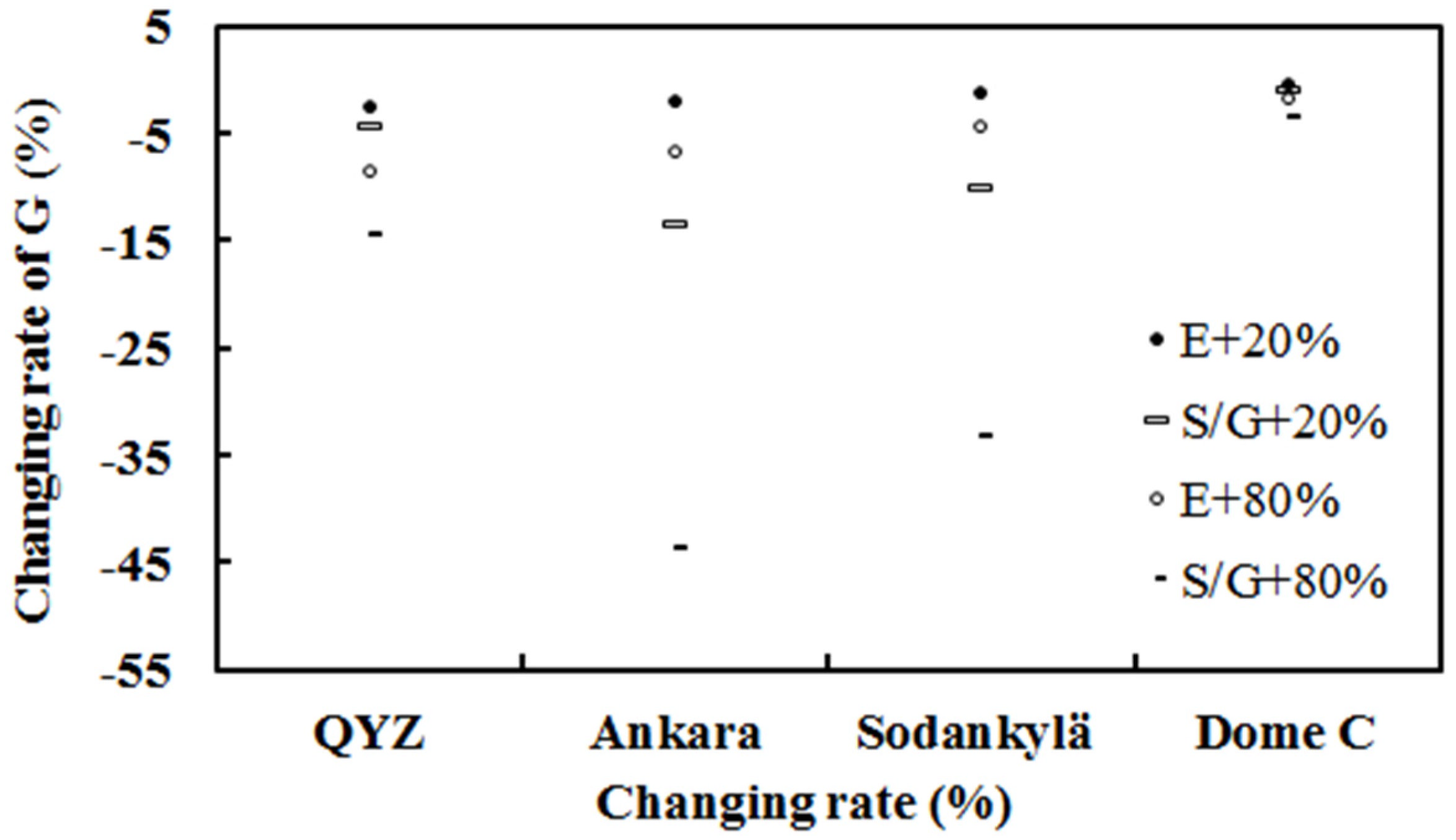
Figure 14.
The averages of m × E, m × (S/G), m2 × E, and m2 × (S/G) at four typical sites.

Figure 15.
Linear (up) and non-linear (bottom) relationships between the increasing rate of air temperature (ΔT, °C in 10 years) and latitude in the winter (left) and summer (right) seasons at some typical sites in China.
Figure 15.
Linear (up) and non-linear (bottom) relationships between the increasing rate of air temperature (ΔT, °C in 10 years) and latitude in the winter (left) and summer (right) seasons at some typical sites in China.
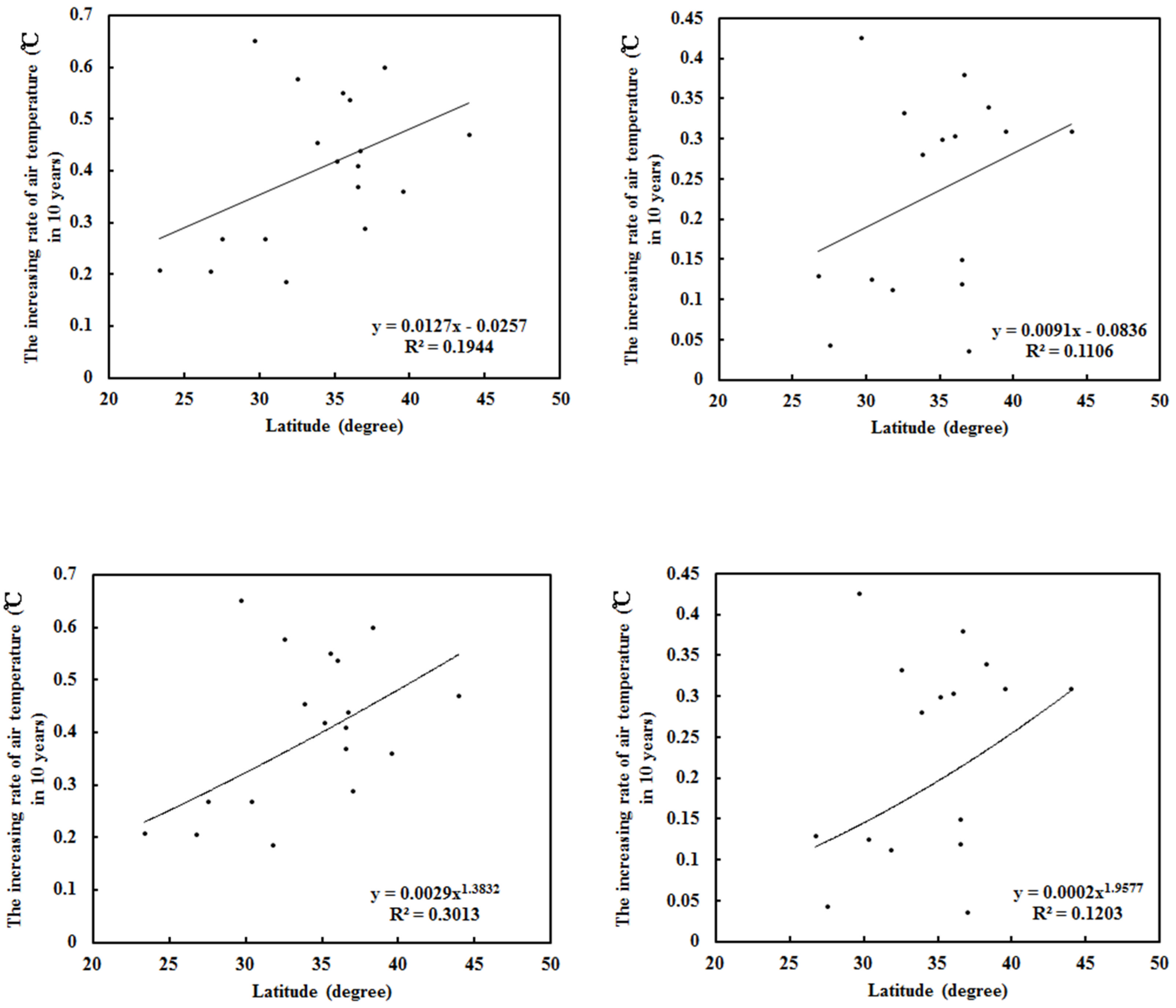
Table 1.
The coefficients and constants for the empirical model of global solar radiation (Equation (1)), determined using measurements in Ankara province in 2017–2018, together with statistical metrics, i.e., coefficient of determination (R2), average and a maximum of the absolute relative bias ( %), NMSE, standard deviations of calculated and observed global solar radiation (σcal and σobs, respectively), the mean bias errors (MAD, in MJ m−2 and %), and the root mean square errors (RMSE, in MJ m−2 and %) (n = 6160).
| A1 | A2 | A0 | R2 | δavg | NMSE | σcal | σobs | MAD | RMSE | ||
|---|---|---|---|---|---|---|---|---|---|---|---|
| (MJ m−2) | (%) | (MJ m−2) | (%) | ||||||||
| 3.587 | 2.977 | −2.013 | 0.916 | 27.14 | 0.025 | 0.914 | 0.955 | 0.199 | 11.38 | 0.265 | 15.14 |
Table 2.
Same as Table 1, but for annual averages of hourly values from 1 January 2017 to 31 December 2019.
Table 2.
Same as Table 1, but for annual averages of hourly values from 1 January 2017 to 31 December 2019.
| Year | δavg | n | NMSE | σcal | σobs | MAD | RMSE | ||
|---|---|---|---|---|---|---|---|---|---|
| MJ m−2 | % | MJ m−2 | % | ||||||
| 2019 | 189.6 | 4323 | 0.065 | 1.10 | 1.05 | 0.243 | 18.47 | 0.327 | 24.82 |
| 2017–2019 | 184.0 | 12,681 | 0.061 | 1.12 | 1.06 | 0.241 | 18.01 | 0.324 | 24.20 |
Table 3.
Seasonal mean values of losses of global solar exposure (MJ m−2) and irradiance (W m−2) caused by absorbing and scattering substances (GLA and GLS), total loss (GL = GLA + GLS) and their contributions to total loss (RLA and RLS, %), and water vapor pressure (E) and S/G, together with annual mean averages of all above variables from 2017 to 2019.
| Season | GLA MJm−2 | GLS MJm−2 | GL MJm−2 | GLA Wm−2 | GLS Wm−2 | GL Wm−2 | RLA % | RLS % | E hPa | S/G |
|---|---|---|---|---|---|---|---|---|---|---|
| Spring | 1.92 | 1.26 | 3.18 | 532.30 | 350.16 | 882.46 | 60.95 | 39.05 | 7.96 | 0.61 |
| Summer | 1.86 | 0.94 | 2.80 | 517.51 | 261.11 | 778.62 | 67.43 | 32.57 | 12.27 | 0.43 |
| Autumn | 2.31 | 1.07 | 3.38 | 640.79 | 297.81 | 938.60 | 69.96 | 30.04 | 8.00 | 0.50 |
| Winter | 2.58 | 1.52 | 4.11 | 717.18 | 423.09 | 1140.3 | 63.82 | 36.18 | 5.90 | 0.77 |
| Average | 2.17 | 1.20 | 3.37 | 601.94 | 333.04 | 934.99 | 65.54 | 34.46 | 8.50 | 0.58 |
Table 4.
Change rate of G (%) due to changes in E or S/G (%), with S/G or E keeping their original values. The change rate of G was computed using (Gcaln − Gcal) × 100/Gcal, where Gcaln is Gcal using new E or S/G, and Gcal is the previous estimation using the original values of E and S/G.
Table 4.
Change rate of G (%) due to changes in E or S/G (%), with S/G or E keeping their original values. The change rate of G was computed using (Gcaln − Gcal) × 100/Gcal, where Gcaln is Gcal using new E or S/G, and Gcal is the previous estimation using the original values of E and S/G.
| E (%) | S/G (%) | |||||||||||||
|---|---|---|---|---|---|---|---|---|---|---|---|---|---|---|
| +20 | +40 | +80 | +160 | −20 | −40 | −80 | +20 | +40 | +80 | +160 | −20 | −40 | −80 | −100 |
| −1.97 | −3.72 | −6.76 | −11.64 | 2.27 | 4.97 | 13.38 | −13.35 | −24.91 | −43.71 | −69.29 | 15.47 | 33.46 | 78.93 | 107.66 |
Table 5.
Averages of E and S/G, change rates of G (%) when E and S/G increase by 20% and 80%, respectively, m × E and m × (S/G), m2 × E and m2 × (S/G) for the four stations (Qianyanzhou (expressed as QYZ), Sodankylä and Dome C in 2013–2016, and Ankara in 2017–2018).
Table 5.
Averages of E and S/G, change rates of G (%) when E and S/G increase by 20% and 80%, respectively, m × E and m × (S/G), m2 × E and m2 × (S/G) for the four stations (Qianyanzhou (expressed as QYZ), Sodankylä and Dome C in 2013–2016, and Ankara in 2017–2018).
| Station | E hPa | S/G | E +20% | S/G +20% | E +80% | S/G +80% | mE | m(S/G) | m2E | m2(S/G) |
|---|---|---|---|---|---|---|---|---|---|---|
| QYZ | 23.96 | 0.71 | −2.48 | −4.41 | −8.53 | −14.39 | 32.65 | 0.97 | 44.47 | 1.32 |
| Ankara | 8.90 | 0.47 | −1.97 | −13.35 | −6.76 | −43.71 | 15.62 | 0.82 | 27.41 | 1.45 |
| Sodankylä | 8.55 | 0.50 | −1.25 | −10.03 | −4.31 | −33.37 | 14.84 | 0.86 | 25.75 | 1.49 |
| Dome C | 0.19 | 0.14 | −0.48 | −0.893 | −1.66 | −3.423 | 0.40 | 0.29 | 0.85 | 0.61 |
Disclaimer/Publisher’s Note: The statements, opinions and data contained in all publications are solely those of the individual author(s) and contributor(s) and not of MDPI and/or the editor(s). MDPI and/or the editor(s) disclaim responsibility for any injury to people or property resulting from any ideas, methods, instructions or products referred to in the content. |
© 2024 by the authors. Licensee MDPI, Basel, Switzerland. This article is an open access article distributed under the terms and conditions of the Creative Commons Attribution (CC BY) license (https://creativecommons.org/licenses/by/4.0/).
Share and Cite
MDPI and ACS Style
Bai, J.; Wan, X.; Arslan, E.; Zong, X. Global Solar Radiation and Its Interactions with Atmospheric Substances and Their Effects on Air Temperature Change in Ankara Province. Climate 2024, 12, 35. https://doi.org/10.3390/cli12030035
AMA Style
Bai J, Wan X, Arslan E, Zong X. Global Solar Radiation and Its Interactions with Atmospheric Substances and Their Effects on Air Temperature Change in Ankara Province. Climate. 2024; 12(3):35. https://doi.org/10.3390/cli12030035
Chicago/Turabian StyleBai, Jianhui, Xiaowei Wan, Erhan Arslan, and Xuemei Zong. 2024. "Global Solar Radiation and Its Interactions with Atmospheric Substances and Their Effects on Air Temperature Change in Ankara Province" Climate 12, no. 3: 35. https://doi.org/10.3390/cli12030035
Note that from the first issue of 2016, this journal uses article numbers instead of page numbers. See further details here.