Statistical Analysis and Modeling of the CO₂ Series Emitted by Thirty European Countries

Abstract

In recent decades, an increase in the earth’s atmospheric temperature has been noticed due to the augmentation of the volume of gases with the greenhouse effect (GHG) released into the atmosphere. To reduce this effect, the European Union’s directives indicate the action directions for reducing these emissions, among which carbon dioxide (CO₂) recorded the highest amount. In this context, the article analyzes the CO₂ series reported in 1990–2021 by 30 European countries. The Kruskal-Wallis test rejected the hypothesis that the series comes from the same underlying distribution. The Anderson-Darling test rejected the normality hypothesis for seven series out of thirty, and Sen’s procedure found a decreasing trend slope only for 17 series. ARIMA models have been built for all individual series. Grouping the series (by the k-means and hierarchical clustering) provided the base for building the Regional series (RegS), which describes the CO₂ pollution evolution over Europe. The advantage of this approach is to provide the synthetic image of the regional evolution of the CO₂ emission volume (mt), incorporating information from 30 series (one for each country) in only one—RegS. It is also shown that selecting the number of clusters involved in building RegS and assessing their stability is essential for the model’s goodness of fit.

1. Introduction

The Intergovernmental Panel on Climate Change (IPCC) [1] shows that the GHG emissions from human activities reached the highest levels compared to the previous 800,000 years. The US Inventory [2] indicates that in 2021, in the USA, the GHG volume exceeded 6340.2 mil mt of CO₂ equivalents, higher by 6% than in 2020 but lower by 17% than in 2005. The GHG emissions from the EU economy rose to 941 mt CO₂ equivalents in the first quarter of 2023 [3].

Carbon dioxide, the GHG with the highest weight in the total GHG (followed by CO₂, NH₄, and N₂H), results from natural and anthropic sources. The first category includes respiration, ocean release, and decomposition. The second is represented by burning fossil fuels, deforestation, industrial production (like the cement industry), and agricultural activities [4,5,6]. Transportation emitted about a quarter of the EU’s CO₂ volume in 2019, of which more than two-thirds were produced by road transportation [4,5]. CO₂ emissions from transportation have increased by 33.5% from 1990 to 2019 in UE [4].

According to the Intergovernmental Panel on Climate Change (IPCC) document [1], the main cause of temperature augmentation from the middle of the twentieth century has been the enormous amount of GHG emitted into the atmosphere. The Sixth Assessment Report of IPCC shows that to limit this increase, immediate measures must be implemented [7,8,9,10]. According to [11,12], natural sinks contribute to removing some GHG from the atmosphere. However, when the GHG volume is high, these gases remain and accumulate for decades or even hundreds of years (like in the case of CO₂). Therefore, conditions to stimulate the natural sinks’ activity must be created, and artificial sinks should be designed to balance the GHG’s effect [12,13,14].

The experimental results show that people’s constant exposure to CO₂ may harm their health [15,16,17,18,19]. The review of Jacobson et al. [20] and the articles on which it is based also highlight some effects of chronic exposure to CO₂, for example, oxidative stress, diminishing cognitive abilities, kidney calcification, bone demineralization, etc. [21]. Moreover, the adverse effects of the CO₂ excess on the ecosystems, plants, and animals are presented in [22,23]. In this context, Hadipoor et al. [24] indicate some measures to control and reduce CO₂ emissions.

Despite the necessity of emissions’ reduction being understood [25,26,27,28,29,30], there exist differences among countries related to carbon emissions’ responsibility [31,32]. So, most studies in the field discuss the responsibility for embodied CO₂ emissions in international trade [25,31]. Some scientists analyzed the results of the international conventions’ implementation [33], while others focused on the source attribution of GHG emissions [34].

Techniques like ARIMA for modeling the CO₂ series from 1972 to 2013 in Bangladesh [35], exponential smoothing and MLP for forecasting the CO₂ series in Pakistan [36], and the use of the Cobb-Douglas function to estimate the CO₂ sectorial amount in the total CO₂ emission in Indonesia [37] proved to be efficient for this purpose. A review of the methods utilized for emphasizing the correlations between the emissions of CO₂, the consumption of energy, and economic growth is presented in [38]. A survey on approaches utilized for modeling the CO₂ emissions from stationary sources, GIS, and economic assessment can be found in [39]. An overview of the CO₂ globally averaged concentrations series since 1830 is performed in [40].

In the context of the climate change negotiations, which started with the adoption of the Convention on Climate Change in 1992, followed by the Kyoto Protocol in 1997, and the launching of the EU’s Emissions Trading System in 2005, the European Union has been a key player in the fight against climate change. Investigating the CO₂ series evolution is essential for assessing the results of implementing the measures for reducing climate change and diminishing its environmental effects [40,41]. Therefore, different articles studied the CO₂ series’ temporal [35,40,42] or spatial [43,44] evolution in different countries, but fewer performed spatiotemporal [45] analyses, mostly for countries in Asia. In this study, we propose such an approach for investigating the trend of the CO₂ series recorded in thirty European countries in Europe. First, we perform a deep statistical analysis, then build models (utilizing the Box–Jenkins methodology) for the series recorded in each country, and test the hypothesis that all series have the same underlying distribution. The rest of this study is dedicated to concisely presenting the regional and temporal evolution of the CO₂ emission series in Europe and incorporating the information collected into one representative series—the Regional series (RegS) — significant from a spatial viewpoint. RegS is constructed using a selection from the 30 series recorded in the studied countries based on two clustering algorithms—k-means and hierarchical clustering [46,47]. Based on our knowledge, this approach is new in the study field.

It is also shown that finding the optimal number of clusters using different selection algorithms and testing the clusters’ stability is essential for obtaining the best RegS. So, even if it appears at a superficial analysis that clustering is the research goal, it is only one of the most critical steps in the proposed algorithm.

2. Materials and Methods

2.1. Data Series

The analyzed data set consists of the CO₂ net emissions (in mt) series recorded from 1990 to 2021 in the EU—27 countries, Iceland, Norway, and Switzerland. The data series was downloaded in an .xlxs form from the official site of the European Union [48] and represents the series sent by the 30 countries to UNFCCC and the EU GHG Monitoring Mechanism. The series has no gaps. The series was processed and represented in Figure 1 on a logarithmic scale for clarity of representation. The international abbreviations of the countries’ names are utilized in this work: AT—Austria, BE—Belgium, BG—Bulgaria, CH—Switzerland, CY—Cyprus, CZ—Czechia, DE—Germany, DK—Denmark, EE—Estonia, EL—Greece, ES—Spain, FI—Finland, FR—France, HR—Croatia, HU—Hungary, IE—Ireland, IS—Island, IT—Italy, LT—Lithuania, LU—Luxembourg, LV—Latvia, MT—Malta, NL—Netherland, NO—Norway, PL—Poland, PT—Portugal, RO—Romania, SE—Sweden, SI—Slovenia, and SK—Slovakia.

2.2. Methodology

The study is split into two parts. The first focuses on evaluating the evolution of the time series recorded in each country and yearly CO₂ series. The second one concerns building RegS.

2.2.1. Study the Time Series Recorded in Each Country

The steps in the individual series analysis are the following:

(1)

Test the hypothesis that the series is Gaussian against the hypothesis that it is not Gaussian by using the Anderson–Darling (AD) test [49].

(2)

Test the homoskedasticity hypothesis against the heteroskedasticity by the Fligner–Killeen (KF) test [50] (since it is less sensitive to the normality violation) [51].

(3)

Perform the Mann–Kendall (MK) [52] to test the randomness hypothesis against the existence of a monotonic trend. If the null is rejected, the slope of a linear trend will be computed by Sen’s [53]. The following series were subject to this analysis:

(a)

The CO₂ series recorded in each country (30 series);

(b)

The total CO₂ emissions during 1990–2021.

(4)

Perform the Augmented Dickey–Fuller (ADF) test [54] to assess the existence of a unit root vs. the time series stationarity for the series from (3).

(5)

Perform the Kruskal–Wallis (K-W) test [55] to test whether the series in a group originates from the same distribution against the alternative that at least one comes from a different distribution. When the null hypothesis was rejected, the post-hoc Dunn’s test [56], with the adjustment proposed by Hochberg [57], was run.

(6)

Modeling the time series from (3) using the ARIMA technique.

Considering a time process ($X_t$), t∈Z, denote by ${∆}^d{X}_t$ the difference of d-th order of $X_t$. ($X_t$) is an autoregressive integrated moving average process, ARIMA (p,d,q), if:

$$\mathsf{\Phi }\left(B\right){∆}^d{X}_t=\mathsf{\Theta }\left(B\right){\epsilon }_t,$$

(1)

where Φ and Θ are polynomials of p and q orders, respectively, with roots higher than 1, and (${\epsilon }_t$), t∈Z is white noise [58].

An autoregressive process of order p, AR (p), is a particular case of ARIMA, with q = d = 0. A moving average process of order q, MA (q), is an ARIMA (0,0,q).

If, after performing the ADF test, the null hypothesis was rejected, then d = 0. Otherwise, one may differentiate the series and perform the ADF test again until the null is rejected. Otherwise, one may differentiate the series and perform again the ADF test until the null is rejected. Thus, d will be equal to the number of differences taken on the series when getting the null rejected. The p and q orders were selected by analyzing the charts of the autocorrelation and partial autocorrelation functions (ACF and PACF, respectively). The model with the lowest value of the Akaike criterion [59] was kept. The Ljung–Box [60] test was used to check that the residuals form white noise.

All tests were performed at a significance level of 0.05. A p-value less than 0.05 computed in a test (except Dunn’s) leads to rejecting the corresponding null hypothesis. In Dunn’s test, the null hypothesis rejection is performed if the p-value < $\mathsf{\alpha }/2$.

2.2.2. Building RegS

The algorithm run for building RegS from the series recorded in the 30 European countries has the following steps [61,62]:

1.

Determine the optimal number of clusters, k, perform the k-means and hierarchical clustering, and choose the best clustering.

The k-means and hierarchical clustering [63,64,65] were utilized to group the series recorded in the 30 countries. The advantages and disadvantages of these techniques are presented in [66], shortly.

The silhouette [67], elbow [68], and gap statistics methods [69] were employed to determine the optimum k for running the k-means algorithm. Sometimes, these techniques do not provide the same k; thus, the study was performed for each possibility, and the best one was selected using some criteria that will be presented in the following.

The ratio WSS (the within-cluster sum of squares) and BSS/TSS (the between-clusters sum of squares by the total sum of squares) were computed to determine the best clustering in the k-means algorithm. The higher the BSS/TSS is, the better is the clustering. A smaller WSS indicates better groupings, as well [70].

Hierarchical clustering is a method whose graphical output is a dendrogram that indicates the series’ hierarchy. The distance between elements is computed in the first stage, and the distance matrix is built. Different distance functions can be used for this purpose, including Euclidean, Manhattan, Hamming, Jaccard, etc. In this study, the first one was utilized.

Hierarchical clustering can be agglomerative or divisive. In the first one utilized here, a cluster is initially created for each element, then, successively, the groups are merged until only one cluster is obtained. The selection of the clusters to be merged at an intermediate step is performed after checking the distances between the couples of clusters. The most similar clusters (couples with the lowest distances between them) are merged. The cluster similarity is defined using different linkage methods, among which are “average”, “complete”, “median”, “ward.D”, “ward.D2”, etc. [65,71]. In the “average” (“complete”) method, the average (maximum) distances between pairs of elements (one from a cluster and the other one from another cluster) are returned. These two methods performed the best on the CO₂ dataset, taking into account the values of the cophenetic correlation coefficient [72,73]. Values greater than 0.9 (between 0.8 and 0.9) indicate a very good (good) clustering quality, whereas less than 0.8 show poor clustering results. After obtaining the clusters, the average Jaccard (AvgJaggard) measures and associated instabilities are computed to verify whether the algorithm (k-means and hierarchical clustering, in this case) provided a satisfactory representation in different groups of the studied dataset. AvgJaggard > 0.85 indicates a high stability of the cluster. AvgJaggard in [0.6, 0.85) (lower than 0.6) shows that the cluster is stable (unstable) [74].

2.

Select the cluster with the highest number of elements, Cl_max. When at least two clusters have this property, Cl_max is the one with the smallest WSS.

3.

Compute RegS, whose elements are the averages of the series from Cl_max. More precisely, the value assigned to year j is the mean of values recorded in the same year in the countries from Cl_max.

4.

Evaluate the modeling errors for each series by subtracting the values of RegS from the recorded values.

5.

Estimate the RegS’s goodness-of-fit of by computing the mean absolute percentage error (MAPE). MAPE was chosen because it is a non-dimensional index that can be utilized for comparing different models.

The R 4.3.2 software (https://www.r-project.org/) was used to perform the study.

3. Results and Discussion

3.1. Analysis of the CO₂ Time Series

The Anderson–Darling test rejected the null hypothesis for the series recorded in BE, DK, EE, ES, FR, HU, IE, IS, IT, LT, MT, NL, PL, PT, SI, SK, and the total CO₂ series. The homoscedasticity hypothesis was rejected for the IS, IT, LT, LU, NO, and SI series.

The MK trend test applied to the total CO₂ series obtained by summing all series values recorded in each country during 1990–2021 rejected the null hypothesis. The nonparametric Sen’s procedure provided a negative slope of −2.9589$\times {10}^7$ for the period 1990–2021. The polynomial trend determined for 1990–2002 has the equation:

$$y_t=-766992t^3+5\times {10}^9{t}^2-5\times {10}^{9}t+6\times {10}^{11} ({\mathrm{R}}^2=0.8144)$$

(2)

and after 2003, it has the equation:

$$y_t=-5.3788\times {10}^{7}t+1.1127\times {10}^{11} ({\mathrm{R}}^2=0.9012),$$

(3)

where t is the time and $y_t$ is the value of the series at the moment t.

Table 1. The p-values in the MK test on the CO₂ series reported by the European countries.

Country	AT	BE	BG	CH	CY	CZ	DE	DK	EE	EL
MK p−val	0.000 (+)	0.000 (−)	0.007 (−)	0.002 (−)	0.001 (+)	0.000 (−)	0.000 (−)	0.000 (−)	0.5703	0.116
Country	ES	FI	FR	HR	HU	IE	IS	IT	LT	LU
p−val	0.783	0.212	0.000 (−)	0.250	0.000 (−)	0.446	0.000 (+)	0.001 (−)	0.003 (−)	0.034 (−)
Country	LV	MT	NL	NO	PL	PT	RO	SE	SI	SK
p−val	0.570	0.043 (−)	0.001 (−)	0.884	0.017 (−)	0.910	0.000 (−)	0.000 (−)	0.062	0.000 (−)

presents the p-values computed in the MK test for the CO₂ series recorded in each country during the study period. If the p-value is less than 0.05, it is accompanied by the sign plus or minus between the brackets, meaning that the slope of the linear trend computed by Sen’s method is positive or negative, respectively. Out of 30 series, the null hypothesis was rejected for 20 s. A positive trend was found for the AT, CY, and IS series, whereas a negative trend was estimated for 17 countries.

The ADF test could not reject the hypothesis of a unit root existence for any series at the significance level of 5%. Therefore, there is not enough evidence for the series stationarity. Therefore, to reach stationarity, some transformations must be employed.

Table 2. ARIMA-type models for the series recorded in each country.

	Model	Coefficient (se)	Drift (se)	Ljung–Box	MAPE
AT	ARIMA (0,1,0)			0.068	9.540
BE	ARIMA (1,1,0)	ar1 = −0.5379 (0.1541)	−823,323.2 (434,892.5)	0.585	2.528
BG	ARIMA (0,1,0)			0.696	10.242
CH	ARIMA (0,1,0)			0.163	3.565
CY	ARIMA (1,2,0)	ar1 = −0.4796 (0.1660)		0.872	3.118
CZ	ARIMA (0,1,0)		−1,672,886.6 (912,138.5)	0.721	3.382
DE	ARIMA (0,1,0)		−13,175,314 (5,529,230)	0.663	2.801
DK	ARIMA (0,1,1)	ma1 = −0.3653 (0.1724)	−1,071,914.1 (530,997.1)	0.863	5.936
EE	ARIMA (1,0,0),mean = 18,424,007 (5,355,966)	ar1 = 0.9194 (0.0809)		0.978	15.576
EL	ARIMA (0,2,1)	ma1 = −0.7087 (0.1233)		0.578	3.755
ES	ARIMA (0,0,0), mean = 240,898,858 (7,123,938)			0.000	13.679
FI	ARIMA (0,0,1) with mean = 30,004,148 (1,645,259)	ma1 = 0.4819 (0.2230)		0.662	19.416
FR	ARIMA (0,1,1)	ma1 = −0.4832 (0.1950)	−3,180,106 (1,285,215)	0.575	2.903
HR	ARIMA (1,0,0), mean = 12,922,689 (1,229,364)	ar1 = 0.7948 (0.0809)		0.889	8.736
HU	ARIMA (0,1,0)		−923,762.9 (441,331.6)	0.429	3.588
IE	ARIMA (1,0,2) with mean = 44,879,052 (2,889,765)	ar1 = 0.8256 (0.0983) ma1 = 0.2435 (0.1239) ma2 = 0.6980 (0.1712)		0.997	2.913
IS	ARIMA (0,1,0)		37689.71 (24201.84)	0.501	1.227
IT	ARIMA (0,1,0)			0.956	3.974
LT	ARIMA (0,1,0)			0.256	27.837
LU	ARIMA (2,0,0) with mean = 9,754,522.1 (622,592.4)	ar1 = 1.1611 (0.1629) ma1 = −0.3443 (0.1769)		0.626	5.342
LV	ARIMA (0,0,1) with mean = 4,189,224.4 (525,627.8)	ma1 = 0.5705 (0.1333)		0.586	258.177
MT	ARIMA (0,1,0)			0.934	6.524
NL	ARIMA (1,2,1)	ar1 = −0.2340 (0.1926) ma1 = 0.8333 (0.1073)		0.567	2.651
NO	ARIMA (1,0,0), mean = 24,099,466 (1,405,598)	ar1 = 0.6871 (0.1205)			9.482
PL	ARIMA (0,1,0)			0.795	3.040
PT	ARIMA (1,0,0), mean = 49,480,302 (3,843,606)	ar1 = 0.6729 (0.1330)		0.945	10.135
RO	ARIMA (0,1,1)	ma1 = 0.5272 (0.1465)	−4,199,933 (2,188,561)	0.569	10.766
SE	ARIMA (0,1,0)			0.714	55.183
SI	ARIMA (0,1,0)			0.356	7.363
SK	ARIMA (0,1,0)		−793,429.1 (483,098)	0.783	6.182

contains the modeling results, as follows:

-

Column 2—the model type;

-

Column 3—the model’s coefficients (when a simple differentiation did not lead to the model) and the corresponding standard error (se) inside the brackets;

-

Column 4—the drift, if it exists, and the standard error (se) of its estimation inside the brackets;

-

The p-value computed in the Ljung–Box test applied to the model’s residual series;

-

The MAPE of the model.

The results from Table 2 indicate that all models except for ES were validated by the Ljung–Box test. Still, relatively high MAPEs were found in those of LV and SE. Therefore, we must find a better approach to model the ES, LV, and SE series. It will be the subject of another article. The AT, BG, CH, CZ, DE, HU, IS, LT, MT, PL, SE, and SK series are described by ARIMA (0,1,0), which is obtained by taking the first-order difference of the raw series. AR(1) models were determined for EE, HR, NO, and PT, AR(2) for LU, and MA(1) for FI and LV. The rest of the series, excluding ES, have models with d = 1 or 2. These findings are in concordance with those of the ADF test.

The model of the total CO₂ series is of ARIMA (0,1,0) with the drift = −3,481,622 (se = 18,455,798) and MAPE = 2.5848. The p-value in the Ljung–Box test is 0.7458.

3.2. Building RegS

The critical step of the algorithm used for building RegS is to determine the optimal number of clusters, k. Different values were found for k—two, three, or one—by the silhouette, the elbow-knee method (Figure 2), and gap statistics, respectively. Since the result provided by the last method is influenced by the outlier existence (Germany, in this case—Figure 1) and the small distances between some clusters [61], it was neglected; thus, the study was performed for the remaining alternatives.

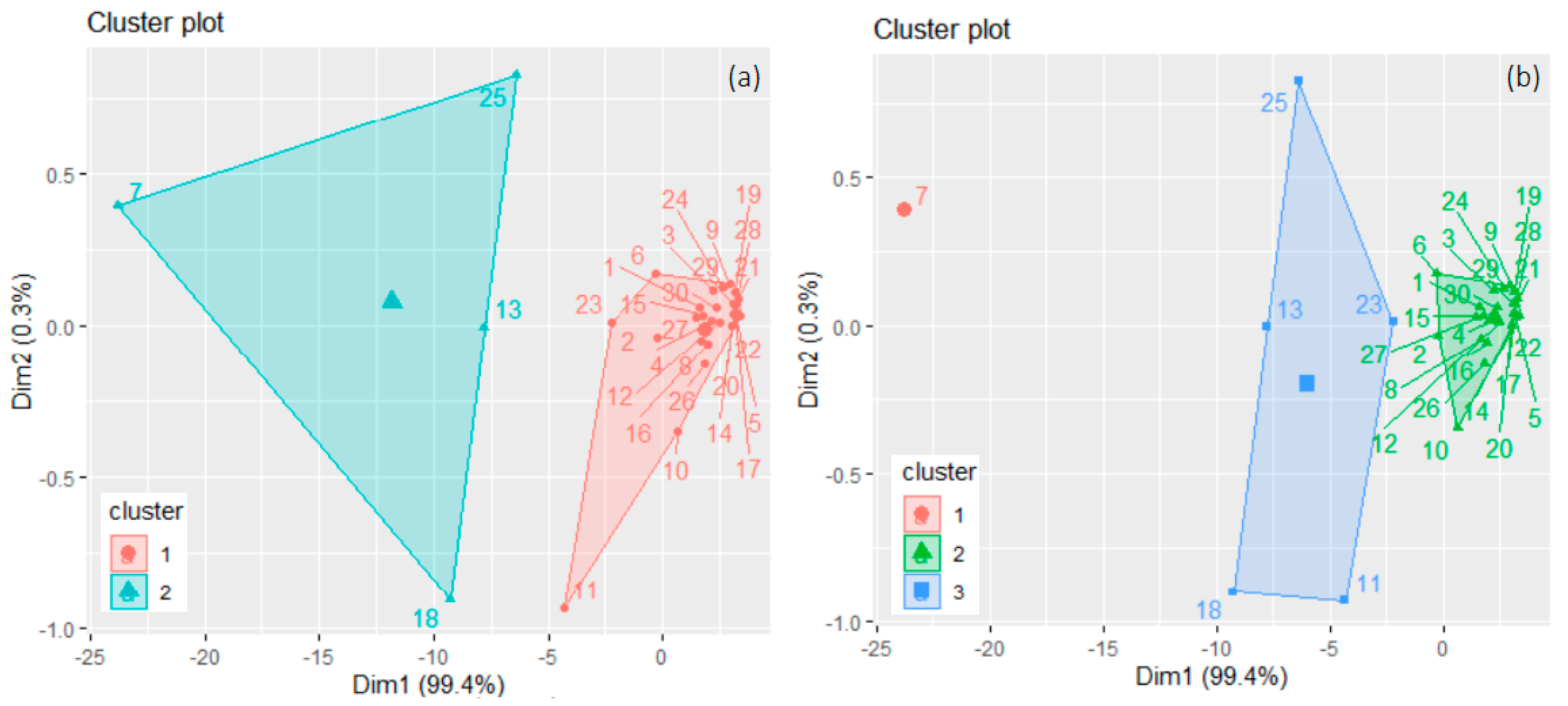
The clusters resulting after running the k-means algorithm are shown in Figure 3a for k = 2 and in Figure 3b for k = 3, where the names of the countries are replaced, for simplicity, by numbers from 1 to 30 assigned from AT to SK (in an alphabetical order).

WSSs are 86.7687 and 197.9709, respectively, and BSS/TSS = 69.3% for k = 2. WSS is high for the second cluster that contains DE(7), FR(13), IT(18), and PL(25). WSS has significantly lower values for k = 3 (0.000, 27.1215, and 34.1752), and BSS/TSS = 93.4%. Thus, the algorithm provides a significantly higher separation between the clusters when k = 3. In this case, Germany (7) forms a single cluster, ES(11), FR(13), IT(18), NL(23), and PL(25) belong to the third cluster, and the rest of the countries form the second one. This output can be explained by the series’ characteristics, like the average emissions levels or the existence of a certain type of trend of the time series in the same cluster. Indeed, the CO₂ emissions in Germany are much higher than those of the countries from the third cluster: ES, FR, IT, NL, and PL. Moreover, the last four mentioned series have a decreasing trend. Still, the groups’ stability must be verified before selecting the best division of the countries in different subsets. The average Jaccard values and the instabilities for the two clusterings are shown in

Table 3. The average Jaccard values and instabilities in the k-means clustering.

k = 2			k = 3
Clusters	AvgJaccard	Instability	Clusters	AvgJaccard	Instability
1	0.7507	0.343	1	0.6445	0.361
2	0.9568	0.000	2	0.9061	0.007
			3	0.8511	0.087

.

When k = 2, the first cluster is stable, and the second one is highly stable. When k = 3, the first is stable, and the other two are highly stable. In both cases, the highest instability is that of the first cluster (that contains Germany). Hierarchical clustering was also formed to cross-validate the above grouping and select the best one.

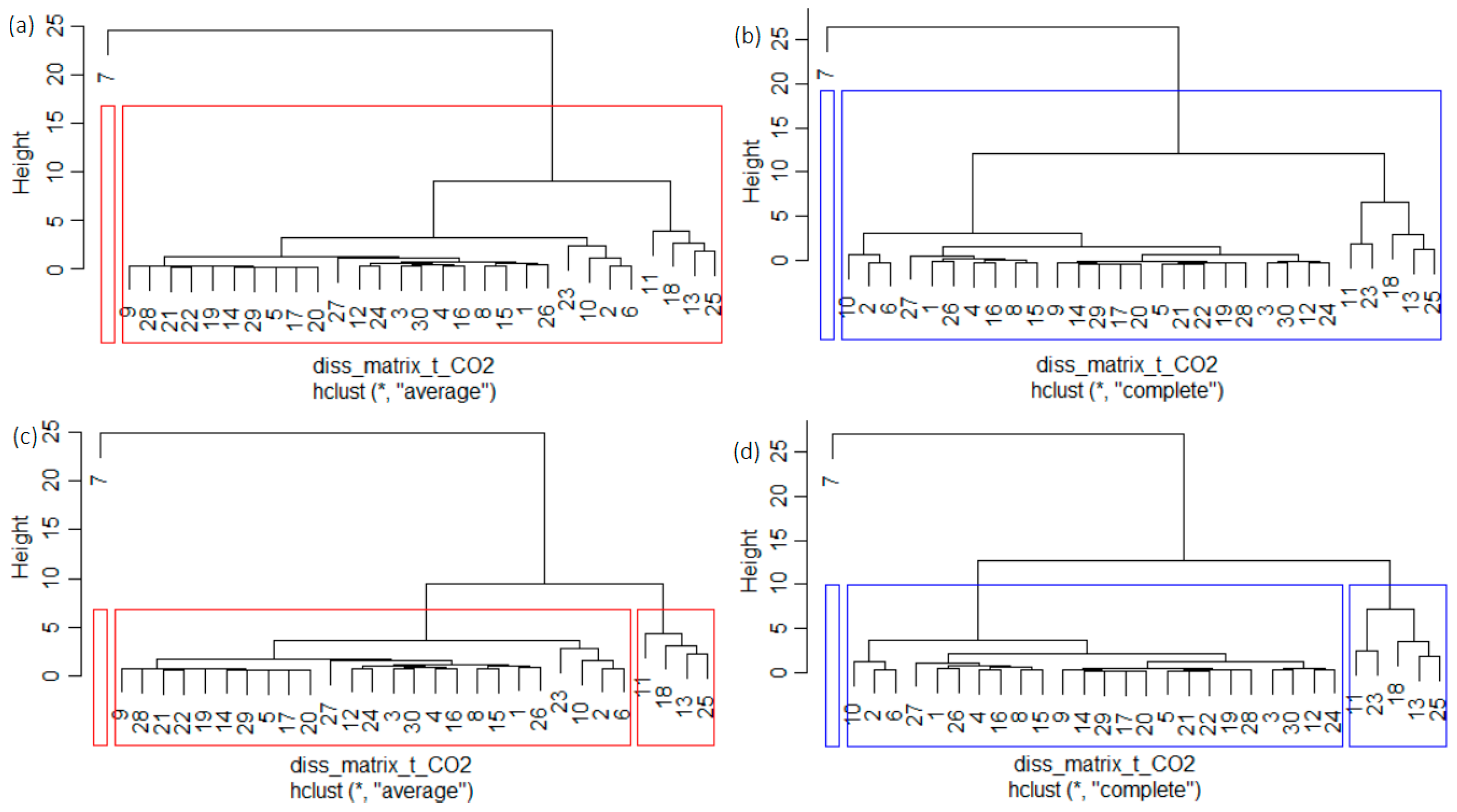
The cophenetic coefficient was computed to choose the linkage method. The highest value (0.9723) was obtained when using the “average”, followed by the “complete” (0.9473), compared to only 0.7474 in the case of “ward.D2”, or 0.7291 in the case of “ward” methods. Therefore, the “average” and “complete” linkage were utilized. The clustering obtained is provided in Figure 4a,b for k = 2 and Figure 4c,d for k = 3.

For k = 2, both methods provided the same clusters. The second cluster contained all countries but Germany. When k = 3, apart from Germany, which forms a cluster, there is a slight difference between the other two clusters when using “average” and “complete” methods (Figure 4c,d). In the first case, ES(11), FR (13), IT(18), and PL(25) belong to a cluster, while in the second one, NL(23) is added.

The clustering obtained by “complete” linkage, containing 1, 24, and 5 elements, coincides with that given by the k-means algorithm (Figure 3b). They cross-validate each other. The average Jaccard indicators computed after bootstrapping are given in

Table 4. The average Jaccard values and instabilities in the hierarchical clustering.

	k = 2			k = 3
	Clusters	AvgJaccard	Instability	Clusters	AvgJaccard	Instability
	1	0.9453	0.000	1	0.9685	0.003
Average	2	0.6320	0.368	2	0.6330	0.367
				3	0.8607	0.100
	1	0.9479	0.000	1	0.9567	0.002
Complete	2	0.6500	0.350	2	0.6520	0.348
				3	0.7994	0.161

.

Considering the ratio BSS/TSS in the k-means algorithm, the average Jaccard values and instabilities in the k-means, and hierarchical clustering, the best choice is k = 3. Indeed, when using “average”, two clusters are highly stable, and one is stable. If “complete” is employed, two clusters are stable, and one is highly stable. Both linkage methods provide good results in terms of AvgJaccard and instability.

That obtained by the “average” is better since the average instability is slightly lower than in the care of the “complete” method. Still, since the results are comparable, for building RegS, both alternatives were used, and the comparison is presented.

Table 5. MAPE (%) in the RegS modeling built using the series form the second cluster. The cluster to which the country belongs is marked inside the bracket, with Roman numerals: I = 1, II = 2, and III = 3.

Country	AT(II)	BE(II)	BG(II)	CH(II)	CY(II)	CZ(II)	DE(I)	DK(II)	EE(II)	EL(II)
MAPE_c	31.37	67.32	10.48	8.98	461.98	68.09	95.61	29.29	162.05	56.28
MAPE_av	22.45	62.46	17.15	7.32	544.39	63.33	94.96	20.99	201.15	49.78
Country	ES(III)	FI(II)	FR(III)	HR(II)	HU(II)	IE(II)	IS(II)	IT(III)	LT(II)	LU(II)
MAPE_c	84.30	35.67	89.35	206.68	27.70	20.23	322.71	90.55	460.03	286.51
MAPE_av	81.98	53.32	87.76	252.04	16.87	13.55	384.98	89.14	545.67	343.94
Country	LV(II)	MT(II)	NL *	NO(II)	PL(III)	PT(II)	RO(II)	SE(II)	SI(II)	SK(II)
MAPE_c	3479.83	1515.61	78.73	59.12	87.70	24.26	37.91	790.94	267.03	13.25
MAPE_av	3989.87	1756.43	75.58	82.63	85.88	16.69	36.49	926.02	321.11	29.31

* Note: NL belongs to the cluster II (III) when using complete (average) method.

contains the MAPE (%). The MAPEs corresponding to the “complete” and “average” are denoted by MAPE_c and MAPE_av, respectively.

The values of MAPE_c (MAPE_av) are in the following intervals: 20 (20) are lower than 100, one (zero) is between 100 and 200, 3 (2) are between 200 and 300, 3 (3) are between 300 and 500, and the rest are higher than 500. The series values from the first and third clusters and most from the second cluster are well estimated. The highest values correspond to the countries with the lowest emissions, among which CY and IS have increasing trends. Considering the average MAPE for all countries (MAPE_c = 298.88, MAPE_av = 342.44), and that the lower the MAPE, the better the fitting is, we can conclude that the best result was obtained using the first linkage method.

To show that building RegS using the cluster with the highest number of elements is the best choice, we also built such a series using the series from the first and last clusters. MAPE was denoted by MAPE_DE (when using the first cluster—DE series), MAPE_c_III (when using the series from the third cluster with the “complete” method), and MAPE_av_III (when using the series from the third cluster with the “average” method). Based on the results from

Table 6. MAPE (%) when building regional series using the cluster I (DE) and III.

Country	AT(II)	BE(II)	BG(II)	CH(II)	CY(II)	CZ(II)	DE(I)	DK(II)	EE(II)	EL(II)
MAPE_DE	1470.27	645.88	2185.87	1999.82	12,765.59	628.38	0	1514.20	5862.92	899.55
MAPE_c_III	495.42	183.73	773.61	698.86	4755.16	177.69	61.84	515.07	2191.58	279.10
MAPE_av_III	440.63	157.82	693.56	625.74	4308.59	152.34	65.33	459.30	1981.18	244.53
Country	ES(III)	FI(II)	FR(III)	HR(II)	HU(II)	IE(II)	IS(II)	IT(III)	LT(II)	LU(II)
MAPE_DE	259.42	2948.87	143.00	6927.44	1550.89	1771.96	9549.77	116.04	12,757.89	81,008.29
MAPE_c_III	35.95	1054.96	7.64	2560.80	529.14	608.88	3564.49	17.93	4820.68	3261.18
MAPE_av_III	23.53	948.93	15.94	2316.76	471.88	543.93	3227.47	25.40	4376.74	2953.39
Country	LV(II)	MT(II)	NL *	NO(II)	PL(III)	PT(II)	RO(II)	SE(II)	SI(II)	SK(II)
MAPE_DE	36,791.50	385.23	3523.23	180.29	1632.33	1504.66	19,918.22	8266.20	2465.86	36,791.50
MAPE_c_III	31,259.28	13,915.38	84.61	1283.56	10.63	557.26	511.89	7706.14	3090.75	878.89
MAPE_av_III	28,253.60	12,639.55	67.68	1156.23	10.35	497.13	457.15	6998.47	2796.41	789.56

* Note: NL belongs to the cluster II (III) when using complete (average) method.

, the first choice is the worst, as it overestimates all the values from the other countries.

Building RegS with the series from the third cluster provides significantly (sometimes more than ten times) higher MAPE than when using the second cluster for this purpose (see MAPE_c_III from Table 6 vs. MAPE_c from Table 5, and MAPE_av_III from Table 6 vs. MAPE_av from Table 5).

The regional series obtained in all cases are depicted in Figure 5, where RegS_c (RegS_av) is the series obtained by using the elements from the cluster with the highest number of elements and the “complete” (“average”) method, DE is the series from the first cluster, and Reg_III_c (Reg_III_av) is the series obtained by using the elements from the cluster third cluster and the “complete” (“average”) method.

Apart from the overall decreasing trend captured by the models, one may note short augmentation periods followed by abrupt decreases, which could be explained by the continuous monitoring and regulations that appeared and were applied to control and restrict CO₂ emissions. Comparing the values from Table 5 and Table 6 with the built regional series (Figure 5), it results a drastic overestimation of the regional evolution of CO₂ series over Europe. So, the best approach is that proposed in the methodology.

Comparing the results from Table 1 with those obtained by the first procedure for the total GHG series recorded in Europe during the same period [47], the following groups of countries are determined as follows:

(a)

Countries (HR, EE, FI, EL, IE, PT, SI, ES) for which the MK test did not reject H₀ for both CO₂ and GHG series, so no significant monotonic trend can be emphasized;

(b)

Countries for which H₀ was rejected and both CO₂ and GHG series have the same type of trend: negative (BE, BG, CH, CZ, DE, DK, FR, HU, IT, LT, LU, NL, PL, RO, SE, and SK) or positive (AT, CY, and IS);

(c)

Countries for which the CO₂ series has a negative slope of the trend, but H₀ was not rejected for the total GHGs series (MT).

(d)

Countries for which H₀ was not rejected, but the GHGs series have a monotonic increasing (LV) or decreasing (NO) trend.

So, most CO₂ and total GHG series trends have a similar pattern. All series evolution but one can be described by ARIMA models. For most series, the correlation between the CO₂ and GHG series (reported by the same country) is above 0.973, except for the Netherlands (0.847) and Norway (0.853).

4. Conclusions

This article studied the CO₂ series reported by 30 countries from 1990 to 2021 and built the RegS using an original algorithm. RegS shows a decreasing trend of CO₂ emissions, whereas, at the individual level, measures should be applied in about half of the countries to achieve the goal of pollution decrement.

Statistical analysis of big data series from trustworthy sources provides the background for making scientifically based decisions on implementing measures for reducing the pollution from anthropic sources and mitigating environmental disasters.

An analogous study will be developed on the CO₂ volume per capita or GDP to assess the relationship between the economy, society, and environment in an interdisciplinary framework. A probabilistic approach to correlations between such variables will provide an in-depth analysis of the causality relationships. Other problems to be addressed are (a) the uncertainty, delays, and inertia in the proposed models; (b) integrating the socio-economic factors into environmental models; and (c) the risk evaluation.

Future research should answer the questions concerning the most appropriate measures and best implantation methods for sustainable development, and how to motivate society members to support actions towards a cleaner production and environment.

References

- IPCC 2014. Contribution of Working Groups I, II and III to the Fifth Assessment Report of the Intergovernmental Panel on Climate Change. Available online: https://www.ipcc.ch/report/ar5/syr/ (accessed on 14 September 2023).
- Inventory of U.S. Greenhouse Gas Emissions and Sinks. Available online: https://www.epa.gov/ghgemissions/inventory-us-greenhouse-gas-emissions-and-sinks (accessed on 16 November 2023).
- EU Economy Greenhouse Gas Emissions: −3% in Q1 2023. Available online: https://ec.europa.eu/eurostat/web/products-eurostat-news/w/ddn-20230816-1#:~:text=In%20the%20first%20quarter%20of,of%20CO2%2Deq (accessed on 14 September 2023).
- CO2 Emissions from Cars: Facts and Figures (Infographics). Available online: https://www.europarl.europa.eu/news/en/headlines/society/20190313STO31218/co2-emissions-from-cars-facts-and-figures-infographics (accessed on 7 August 2023).
- IEA. CO2 Emissions from Fuel Combustion; IEA: Paris, France, 2019. [Google Scholar] [CrossRef]
- Greenhouse Gas Emissions. Sources of Greenhouse Gas Emissions. Available online: https://www.epa.gov/ghgemissions/sources-greenhouse-gas-emissions (accessed on 7 July 2023).
- IPCC. Climate Change 2022: Mitigation of Climate Change; Cambridge University Press: Cambridge, UK, 2022. [Google Scholar]
- Paris Agreement. In Report of the Conference of the Parties to the United Nations Framework Convention on Climate Change (21st Session, 2015: Paris); HeinOnline: Paris, France, 2015.
- Calotă, R.; Antonescu, N.N.; Stănescu, D.-P.; Năstase, I. The Direct Effect of Enriching the Gaseous Combustible with 23% Hydrogen in Condensing Boilers’ Operation. Energies 2022, 15, 9373. [Google Scholar] [CrossRef]
- Antonescu, N.N.; Stănescu, D.-P.; Calotă, R. CO2 Emissions Reduction through Increasing H2 Participation in Gaseous Combustible—Condensing Boilers Functional Response. Appl. Sci. 2022, 12, 3831. [Google Scholar] [CrossRef]
- Denman, K.L.; Brasseur, G.; Chidthaisong, A.; Ciais, P.; Cox, P.M.; Dickinson, R.E.; Hauglustaine, D.; Heinze, C.; Holland, E.; Jacob, D.; et al. Couplings Between Changes in the Climate System and Biogeochemistry. In Climate Change 2007: The Physical Science Basis. Contribution of Working Group I to the Fourth Assessment Report of the Intergovernmental Panel on Climate Change; Cambridge University Press: Cambridge, UK; New York, NY, USA, 2007. [Google Scholar]
- Saini, M.; Saini, S.K. Identification of Major Sinks of Greenhouse Gases. In Greenhouse Gases: Sources, Sinks and Mitigation; Sonwani, S., Saxena, P., Eds.; Springer: Singapore, 2022; pp. 39–62. [Google Scholar]
- Greenhouse Gas Removal Methods and Their Potential UK Deployment. 2021. Available online: https://assets.publishing.service.gov.uk/government/uploads/system/uploads/attachment_data/file/1026988/ggr-methods-potential-deployment.pdf (accessed on 14 September 2023).
- Ming, T.; de Richter, R.; Oeste, F.D.; Tulip, R.; Caillol, S. A nature-based negative emissions technology able to remove atmospheric methane and other greenhouse gases. Atmos. Pollut. Res. 2021, 12, 101035. [Google Scholar] [CrossRef]
- Naiyer, S.; Abbas, S.S. Effect of Greenhouse Gases on Human Health. In Greenhouse Gases: Sources, Sinks and Mitigation; Sonwani, S., Saxena, P., Eds.; Springer: Singapore, 2022; pp. 85–106. [Google Scholar]
- Hajtar, L.; Herczeg, L. Influence of carbon-dioxide concentration on human well-being and intensity of mental work. Időjárás 2012, 116, 145–169. [Google Scholar]
- Satish, U.; Mendell, M.J.; Shekhar, K.; Hotchi, T.; Sullivan, D.; Strufert, S.; Fisk, W.J. Is CO2 an indoor pollutant? Direct effects of low-to-moderate CO2 concentrations on human decision-making performance. Environ. Health Perspect. 2012, 120, 1671–1677. [Google Scholar] [CrossRef] [PubMed]
- Allen, J.G.; MacNaughton, P.; Satish, U.; Santanam, S.; Vallarino, J.; Spengler, J.D. Associations of cognitive function scores with carbon dioxide, ventilation, and volatile organic compound exposures in office workers: A controlled exposure study of green and conventional office environment. Environ. Health Perspect. 2016, 124, 805–812. [Google Scholar] [CrossRef] [PubMed]
- Snow, S.; Boyson, A.S.; Paas, K.H.W.; Gough, H.; King, M.-F.; Barlow, J.; Noakes, C.J.; Schraefel, M.C. Exploring the physiological, neurophysiological and cognitive performance effects of elevated carbon dioxide concentrations indoors. Build. Environ. 2019, 156, 243–252. [Google Scholar] [CrossRef]
- Jacobson, T.A.; Kler, J.S.; Hernke, M.T.; Braun, R.K.; Meyer, K.C.; Funk, W.E. Direct human health risks of increased atmospheric carbon dioxide. Nat. Sustain. 2019, 2, 691–701. [Google Scholar] [CrossRef]
- Smith, D. Is Carbon Dioxide Harmful to People? Available online: https://learn.kaiterra.com/en/air-academy/is-carbon-dioxide-harmful-to-people (accessed on 15 September 2023).
- Hunter, P. The impact of CO2. The global rise in the levels of CO2 is good for trees, bad for grasses and terrible for corals. EMBO Rep. 2007, 8, 1104–1106. [Google Scholar] [CrossRef] [PubMed]
- Ehleringer, J.R.; Cerling, T.; Dearing, M.D. A History of Atmospheric CO2 and Its Effects on Plants, Animals, and Ecosystems; Ecological Studies 177; Springer: Berlin/Heidelberg, Germany, 2005. [Google Scholar]
- Hadipoor, M.; Keivanimehr, F.; Baghban, A.; Reza Ganjali, M.; Habibzadeh, S. Chapter 24—Carbon dioxide as a main source of air pollution: Prospective and current trends to control. In Sorbents Materials for Controlling Environmental Pollution; Núñez-Delgado, A., Ed.; Elsevier: Amsterdam, The Netherlands, 2021; pp. 623–688. [Google Scholar]
- Wang, T.; Chen, Y.; Zeng, L. Spatial-Temporal Evolution Analysis of Carbon Emissions Embodied in Inter-Provincial Trade in China. Int. J. Environ. Res. Public Health 2022, 19, 6794. [Google Scholar] [CrossRef]
- Li, Y.L.; Chen, B.; Chen, G.Q. Carbon network embodied in international trade: Global structural evolution and its policy implications. Energy Policy 2020, 139, 11131. [Google Scholar] [CrossRef]
- Chiritescu, R.-V.; Luca, E.; Iorga, G. Observational study of major air pollutants over urban Romania in 2020 in comparison with 2019. Rom. Rep. Phys. 2024, 76, 702. [Google Scholar]
- Dumitru, A.; Olaru, E.-A.; Dumitru, M.; Iorga, G. Assessment of air pollution by aerosols over a coal open-mine influenced region in southwestern Romania. Rom. J. Phys. 2024, 69, 801. [Google Scholar]
- Bărbulescu, A.; Dumitriu, C.S.; Popescu-Bodorin, N. On the aerosol optical depth series in the Arabian Gulf region. Rom. J. Phys. 2022, 67, 814. [Google Scholar]
- Bărbulescu, A.; Dumitriu, C.S.; Popescu-Bodorin, N. Assessing atmospheric pollution and its impact on the human health. Atmosphere 2022, 13, 938. [Google Scholar] [CrossRef]
- Ullah, I.; Ali, S.; Shah, M.H.; Yasim, F.; Rehman, A.; Al-Ghazali, B.M. Linkages between Trade, CO2 Emissions and Healthcare Spending in China. Int. J. Environ. Res. Public Health 2019, 16, 4298. [Google Scholar] [CrossRef] [PubMed]
- Jakob, M.; Marschinski, R. Interpreting trade-related CO2 emission transfers. Nat. Clim. Chang. 2013, 3, 19–23. [Google Scholar] [CrossRef]
- Slechten, A.; Verardi, V. Assessing the Effectiveness of Global Air-Pollution Treaties on CO2 Emissions; Working Papers 64981625; Lancaster University Management School, Economics Department: Lancaster, UK, 2014. [Google Scholar]
- Lindenmaier, R.; Dubey, M.K.; Henderson, B.G.; Butterfield, Z.T.; Herman, J.R.; Rahn, T.; Lee, S. Multiscale observations of CO2, and pollutants at Four Corners for emission verification and attribution. Proc. Nat. Acad. Sci. USA 2014, 111, 8386–8391. [Google Scholar] [CrossRef] [PubMed]
- Budiono, R.; Juahir, H.; Mamat, M.; Sukono; Supian, S.; Nurzaman, M. Modeling and analysis of CO2 emissions in million tons of sectoral greenhouse gases in Indonesia. IOP Conf. Ser. Mat. Sci. Eng. 2019, 621, 012020. [Google Scholar] [CrossRef]
- Debone, D.; Pazini Leite, V.; Georges El Khouri Miraglia, S. Modelling approach for carbon emissions, energy consumption and economic growth: A systematic review. Urban Clim. 2021, 37, 100849. [Google Scholar] [CrossRef]
- Yousefi-Sahzabi, A.; Sasaki, K.; Djamaluddin, I.; Yousefi, H.; Sugai, Y. GIS modeling of CO2 emission sources and storage possibilities. Energy Proceed. 2011, 4, 2831–2838. [Google Scholar] [CrossRef]
- Bâki iz, H. The evolution of large-scale variations in globally averaged atmospheric CO2 concentrations since 1830. All Earth 2022, 34, 16–26. [Google Scholar]
- Hansen, J.; Sato, M.; Kharecha, P.; Beerling, D.; Berner, R.; Masson-Delmotte, V.; Pagani, M.; Raymo, M.; Royer, D.L.; Zachos, J.C. Target Atmospheric CO2: Where Should Humanity Aim? Available online: https://arxiv.org/ftp/arxiv/papers/0804/0804.1126.pdf (accessed on 15 September 2023).
- Rahman, A.; Mahmudul Hasan, M.M. Modeling and Forecasting of Carbon Dioxide Emissions in Bangladesh Using Autoregressive Integrated Moving Average (ARIMA) Models. Open J. Stat. 2017, 7, 560–566. [Google Scholar] [CrossRef]
- Tawiah, K.; Daniyal, M.; Qureshi, M. Pakistan CO2 Emission Modelling and Forecasting: A Linear and Nonlinear Time Series Approach. J. Environ. Public Health 2023, 2023, 5903362. [Google Scholar] [CrossRef] [PubMed]
- Chang, S.C.; Lee, C.T. Evaluation of the temporal variations of air quality in Taipei City, Taiwan, from 1994 to 2003. J. Environ. Manag. 2008, 86, 627–635. [Google Scholar] [CrossRef] [PubMed]
- Kuttippurath, J.; Peter, R.; Singh, A.; Raj, S. The increasing atmospheric CO2 over India: Comparison to global trends. iScience 2022, 25, 104863. [Google Scholar] [CrossRef] [PubMed]
- Zhou, Y.; Zhang, J.; Hu, S. Regression analysis and driving force model building of CO2 emissions in China. Sci. Rep. 2021, 11, 6715. [Google Scholar] [CrossRef]
- Jiang, P.; Gong, X.; Yang, Y.; Tang, K.; Zhao, Y.; Liu, S.; Liu, L. Research on spatial and temporal differences of carbon emissions and influencing factors in eight economic regions of China based on LMDI model. Sci. Rep. 2023, 13, 7965. [Google Scholar] [CrossRef]
- Bărbulescu, A.; Nazzal, Y.; Howari, F. Statistical analysis and estimation of the regional trend of aerosol size over the Arabian Gulf Region during 2002–2016. Sci. Rep. 2018, 8, 9571. [Google Scholar] [CrossRef]
- Bărbulescu, A.; Postolache, F. New approaches for modeling the regional pollution in Europe. Sci. Total Environ. 2021, 753, 141993. [Google Scholar] [CrossRef]
- EEA Greenhouse Gases—Data Viewer. Available online: https://www.eea.europa.eu/data-and-maps/data/data-viewers/greenhouse-gases-viewer (accessed on 15 June 2023).
- Anderson, T.W.; Darling, D.A. Asymptotic theory of certain “goodness of fit” criteria based on stochastic processes. Ann. Math. Stat. 1952, 23, 193–212. [Google Scholar] [CrossRef]
- Fligner, M.A.; Killeen, T.J. Distribution-free two-sample tests for scale. J. Am. Stat. Assoc. 1976, 71, 210–213. [Google Scholar] [CrossRef]
- Conover, W.J.; Johnson, M.E.; Johnson, M.M. A comparative study of tests for homogeneity of variances, with applications to the outer continental shelf biding data. Technometrics 1981, 23, 351–361. [Google Scholar] [CrossRef]
- Kendall, M.G. Rank Correlation Methods, 4th ed.; Charles Griffin: London, UK, 1975. [Google Scholar]
- Sen, P.K. Estimates of the regression coefficient based on Kendall’s tau. J. Am. Stat. Assoc. 1968, 63, 1379–1389. [Google Scholar] [CrossRef]
- Fuller, W.A. Introduction to Statistical Time Series; John Wiley and Sons: New York, NY, USA, 1976. [Google Scholar]
- Kruskal, W.H.; Wallis, W.A. Use of ranks in one-criterion variance analysis. J. Am. Stat. Assoc. 1952, 47, 583–621. [Google Scholar] [CrossRef]
- Dunn, O.J. Multiple comparisons using rank sums. Technometrics 1964, 6, 241–252. [Google Scholar] [CrossRef]
- Hochberg, Y. A sharper Bonferroni procedure for multiple tests of significance. Biometrika 1988, 75, 800–802. [Google Scholar] [CrossRef]
- Brockwell, P.J.; Davis, R.A. Introduction to Time Series and Forecasting; Springer International Publishing: Cham, Switzerland, 2016. [Google Scholar]
- Akaike, H. Time series analysis and control through parametric models. In Applied Time Series Analysis; Findley, D.F., Ed.; Academic Press: New York, NY, USA, 1978. [Google Scholar]
- Ljung, G.M.; Box, G.E.P. On a Measure of a Lack of Fit in Time Series Models. Biometrika 1978, 65, 297–303. [Google Scholar] [CrossRef]
- Bărbulescu, A.; Postolache, F.; Dumitriu, C.Ș. Estimating the precipitation amount at regional scale using a new tool, Climate Analyzer. Hidrology 2021, 8, 125. [Google Scholar] [CrossRef]
- Bărbulescu, A. On the Regional Temperature Series Evolution in the South-Eastern Part of Romania. Appl. Sci. 2023, 13, 3904. [Google Scholar] [CrossRef]
- K-Mean: Getting the Optimal Number of Clusters. Available online: https://www.analyticsvidhya.com/blog/2021/05/k-mean-getting-the-optimal-number-of-clusters/ (accessed on 16 June 2023).
- Hierarchical Clustering in, R. Available online: https://www.datacamp.com/tutorial/hierarchical-clustering-R (accessed on 18 June 2023).
- Kassambara, A. Practical Guide to Cluster Analysis in R. Unsupervised Machine Learning. Available online: https://www.datanovia.com/en/product/practical-guide-to-cluster-analysis-in-r/ (accessed on 10 May 2023).
- Daburra, I. K-Means Clustering: Algorithm, Applications, Evaluation Methods, and Drawbacks. Available online: https://towardsdatascience.com/k-means-clustering-algorithm-applications-evaluation-methods-and-drawbacks-aa03e644b48a (accessed on 18 June 2023).
- Rousseeuw, P. Silhouettes: A Graphical Aid to the Interpretation and Validation of Cluster Analysis. J. Comput. Appl. Math. 1987, 20, 53–65. [Google Scholar] [CrossRef]
- Thorndike, R.L. Who belongs in the family? Psychometrika 1953, 18, 267–276. [Google Scholar] [CrossRef]
- Löhr, T. K-Means Clustering and the Gap-Statistics. Available online: https://towardsdatascience.com/k-means-clustering-and-the-gap-statistics-4c5d414acd29 (accessed on 16 June 2023).
- Madsen, B.E.; Browning, S.R. A Groupwise Association Test for Rare Mutations Using a Weighted Sum Statistic. PLoS Genet. 2009, 5, e1000384. [Google Scholar] [CrossRef]
- Sokal, R.R.; Rohlf, F.J. The comparison of dendrograms by objective methods. Taxon 1962, 11, 33–40. [Google Scholar] [CrossRef]
- Farris, J.S. On the cophenetic correlation coefficient. System. Zool. 1969, 18, 279–285. [Google Scholar] [CrossRef]
- Myrphy, P. Clustering Data in R. Available online: https://rstudio-pubs-static.s3.amazonaws.com/599072_93cf94954aa64fc7a4b99ca524e5371c.html (accessed on 30 June 2023).
- Soetewey, A. Stats and R. The Complete Guide to Clustering Analysis: K-Means and Hierarchical Clustering by Hand and in R. Available online: https://statsandr.com/blog/clustering-analysis-k-means-and-hierarchical-clustering-by-hand-and-in-r/ (accessed on 20 June 2023).
Figure 1.
The annual CO2 series [mt] during 1990–2021, represented in a log10 scale.
Figure 2.
The optimal number of clusters determined by (left) the silhouette and (right) the elbow method for the CO2 series recorded in the European countries.
Figure 3.
Results of the k-means algorithm for grouping the series recorded in the European countries when (a) k = 2 and (b) k = 3. Numbers from 1 to 30 are assigned to the countries in the alphabetical order of names’ abbreviations.
Figure 4.
Hierarchical clustering (a) k = 2 and “average” method; (b) k = 2 and “complete” method; (c) k = 3 and “average” method, (d) k = 3 and “complete” method. The countries are numbered from 1—AT to 30—SK, in the alphabetical order of the countries’ names’ abbreviations.
Figure 5.
RegS for CO2 series.