Article

Seasonal Drought Forecasting for Latin America Using the ECMWF S4 Forecast System

1
European Commission, Joint Research Centre, 21027 Ispra, Italy
2
Space4Environment, L-6947 Niederanven, Luxemburg
3
Instituto Dom Luiz, Faculdade de Ciências, Universidade de Lisboa, 1749-016 Lisbon, Portugal
*
Author to whom correspondence should be addressed.
Climate 2018, 6(2), 48; https://doi.org/10.3390/cli6020048
Submission received: 4 May 2018 / Revised: 28 May 2018 / Accepted: 31 May 2018 / Published: 1 June 2018
(This article belongs to the Special Issue Climate and Atmospheric Dynamics and Predictability)

Abstract

:
Meaningful seasonal prediction of drought conditions is key information for end-users and water managers, particularly in Latin America where crop and livestock production are key for many regional economies. However, there are still not many studies of the feasibility of such a forecasts at continental level in the region. In this study, precipitation predictions from the European Centre for Medium Range Weather (ECMWF) seasonal forecast system S4 are combined with observed precipitation data to generate forecasts of the standardized precipitation index (SPI) for Latin America, and their skill is evaluated over the hindcast period 1981–2010. The value-added utility in using the ensemble S4 forecast to predict the SPI is identified by comparing the skill of its forecasts with a baseline skill based solely on their climatological characteristics. As expected, skill of the S4-generated SPI forecasts depends on the season, location, and the specific aggregation period considered (the 3- and 6-month SPI were evaluated). Added skill from the S4 for lead times equaling the SPI accumulation periods is primarily present in regions with high intra-annual precipitation variability, and is found mostly for the months at the end of the dry seasons for 3-month SPI, and half-yearly periods for 6-month SPI. The ECMWF forecast system behaves better than the climatology for clustered grid points in the North of South America, the Northeast of Argentina, Uruguay, southern Brazil and Mexico. The skillful regions are similar for the SPI3 and -6, but become reduced in extent for the severest SPI categories. Forecasting different magnitudes of meteorological drought intensity on a seasonal time scale still remains a challenge. However, the ECMWF S4 forecasting system does capture the occurrence of drought events for the aforementioned regions and seasons reasonably well. In the near term, the largest advances in the prediction of meteorological drought for Latin America are obtainable from improvements in near-real-time precipitation observations for the region. In the longer term, improvements in precipitation forecast skill from dynamical models, like the fifth generation of the ECMWF seasonal forecasting system, will be essential in this effort.

1. Introduction

Drought is a recurring and extreme climate event that originates in a temporary water deficit and may be related to a lack of precipitation, soil moisture, streamflow, or any combination of the three taking place at the same time [1]. Drought differs from other hazard types in several ways. First, unlike other geophysical hazards that occur along well defined areas (i.e., floods, earthquakes, landslides), drought can occur anywhere with the exception of desert regions and extremely cold areas where it does not have meaning [2,3]. Secondly, drought develops slowly, resulting from a prolonged period (from weeks to years) of precipitation that is below the average, or expected, value at a particular location [4].
To improve drought mitigation, different indicators are used to trigger a drought warning [1,5]. While an indicator is a derived variable for identifying and assessing different drought types, a trigger is a threshold value of the indicator used to determine the onset, intensity or end of a drought, as well as the timing to implement proper drought response actions [6,7]. Since precipitation is one of the most important inputs to a watershed system and provides a direct measurement of water supply conditions over different timescales, several commonly used drought indicators rely on precipitation measurements only [4]. Among them, the Standardized Precipitation Index (SPI) of [8] is certainly the most prominent; it has been recommended by the World Meteorological Organization (WMO) for characterizing the onset, end, duration and severity of drought events deriving from precipitation deficiencies taking place at different accumulation periods and occurring at different stages of a same hydro-meteorological anomaly [9].
The immediate consequences of short-term droughts (i.e., a few weeks duration) are, for example, a fall in crop production, poor pasture growth and a decline in fodder supplies from crop residues, whereas prolonged water shortages (e.g., of several months or years duration) may, among others, lead to a reduction in hydro-electrical production and an increase of forest fire occurrences [10]. Therefore, skillful predictions of the onset and end of a drought a few months in advance will benefit a variety of sectors by allowing sufficient lead time for drought mitigation efforts. Indeed, drought forecasting is nowadays a critical component of drought hydrology science, which plays a major role in drought risk management, preparedness and mitigation.
It has been demonstrated that droughts can be forecasted using stochastic or neural networks [11,12]. While [13] demonstrated that these type of forecast can provide “reasonably good agreement for forecasting with 1 to 2 months lead times”, they do not quantify the improvement of these methods with respect to using probabilistic forecasts of the precipitation fields. Forecasts of droughts can also be produced using deterministic numerical weather prediction models. However, such forecasts are highly uncertain due to the chaotic nature of the atmosphere, which is particularly strong on a sub-seasonal timescale [14].
As an alternative, ensemble prediction systems that forecast multiple scenarios of future weather have considerably evolved over recent years. Indeed, the routine generation of global seasonal climate forecasts coupled with advances in near-real-time monitoring of the global climate has now allowed for testing the feasibility of generating global drought forecasts operationally. Systems to monitor drought around the globe are described in [7] for meteorological drought and in [15] for hydrologic and agricultural conditions. For example, Yuan et al. [16] used seasonal precipitation forecasts from the North American Multi-Model Ensemble (NMME) and other coupled ocean-land-atmosphere general circulation models (GCMs) to examine the predictability of drought onset around the globe based on the SPI. For the global domain, they found only a modest increase in the forecast probability of drought onset relative to baseline expectations when using the GCM forecasts. Hao et al. [17] described the Global Integrated Drought Monitoring and Prediction System (GIDMaPS) that uses three drought indicators. The forecasting component of their system relies on a statistical approach based on an ensemble streamflow prediction (ESP) methodology. Dutra et al. [18,19] generated global forecasts of 3-, 6-, and 12-month SPI by combining seasonal precipitation reforecasts from the European Centre for Medium-Range Weather Forecasts (ECMWF) System 4 (S4) with precipitation observations from the Global Precipitation Climatology Centre (GPCC) and, alternatively, the ECMWF Interim Reanalysis. They reported on several verification metrics for the SPI forecasts for 18 regions around the globe. Using the same definition as [16], they found that the ECMWF S4 provides useful skill in predicting drought onset in several regions, and the skill is largely derived from El Niño-Southern Oscillation (ENSO) teleconnections. However, they also found that in many regions is difficult to improve on “climatological” forecasts. Recently, Spennemann et al. [20] studied the performance and uncertainties of seasonal soil moisture and precipitation anomalies (SPI) forecasts over Southern South America by means of Climate Forecast System, version 2 (CFSv2). Their results show that both SPI and standardized soil moisture anomalies forecast skills are regionally and seasonally dependent. In general, a fast degradation of the forecast skill is observed as the lead time increases, resulting in almost no added value with regard to climatology at lead times longer than 3 months. However, they note that the forecasts have a higher skill for dry events if compared with wet events.
In this study, we build on the work of [18,19] by considering the ECMWF S4 ensemble framework to generate seasonal forecasts of the SPI, and perform their verification against corresponding SPI from precipitation observations of the GPCC over Latin America. Drought is viewed from a meteorological perspective, and seasonal forecasts of the 3- and 6-month SPI (SPI3 and SPI6) are generated and verified on a monthly basis for the hindcast period of 1981–2010.
While the focus of the work is on the prediction of meteorological drought, the study assesses two fundamental constraints in generating reliable regional drought predictions that will arise whether using the reported method or any other approach (e.g., land surface modeling): (1) the accuracy of summary statistics (e.g., mean, median, percentile) at predicting a seasonal drought from the members of the ensemble forecasting system; and (2) the skill of probabilistic categorical predictions of seasonal drought from the members of the ensemble forecasting system.

2. Study Area, Datasets and Methods

The study area covers the whole South-Central America region (the domain of analysis is limited to land surface grid points between 56° S–35° N, 33°–128° W). South-Central America spans a vast range of latitudes and has a wide variety of climates. It is characterized largely by humid and tropical conditions, but important areas have been extremely affected by meteorological droughts in the past [21,22,23] and the climate change scenarios foresee an increased frequency of these events for the region [24,25]. Given the significant reliance of South-Central American economies on rainfed agricultural yields (rainfed crops contribute more than 80% of the total crop production in South-Central America), and the exposure of agriculture to a variable climate, there is a large concern in the region about present and future climate and climate-related impacts [26]. South-Central American countries have an important percentage of their GDP in agriculture (10% average, [27]), and the region is a net exporter of food globally, accounting for 11% of the global value. According to the agricultural statistics supplied by the United Nations Food and Agriculture Organization [27], 65% of the world production of corn and more than 90% of the world production of soybeans occurs in Argentina, Brazil, the United States and China. The productivity of these crops is expected to decrease in the extensive plains located in middle and subtropical latitudes of South-America (e.g., Brazil and Argentina), leading to a reduction in the worldwide productivity of cattle farming and having adverse consequences for global food security [28,29].

2.1. Forecasts: The ECMWF Seasonal Forecast System (S4)

In this study, we use the ECMWF seasonal forecast system 4 (hereafter S4; [30]) to forecast 3- and 6-month SPI. The S4 is a dynamical forecast system based on an atmospheric-ocean coupled model, which has been operational at ECMWF since 2011 and is launched once a month (on the first day of the month). The 2011 version of the forecast model has 91 vertical levels, lead times up to 13 months, and a resolution of T255 (80 km). It provides back integrations (hindcast) with 15/51 member ensemble (number depends on month) for every month from 1980 onwards. Molteni et al. [30] provide a detailed overview of S4 performance. For the comparison with the GPCC observations, the S4 has been re-gridded to 1.0° latitude/longitude grid spacing, and daily precipitation values over its hindcast period (1981–2010) have been aggregated to monthly values. The ability of the probabilistic model to accurately forecast seasonal drought conditions has been evaluated up to 6 months of lead time. In addition to the dynamical seasonal forecasts and in order to test whether the forecasts perform better than a benchmark, a set of climatological forecasts (CLM) were also generated by randomly sampling past years from the reference data set to match the number of ensemble members in the hindcast, as depicted in [19].

2.2. Observations: The GPCC Full Data Reanalysis Version 6.0

In this study, monthly precipitation totals at 1.0° latitude/longitude grid spacing from the Full Data Reanalysis Monthly Product Version 6.0 of the GPCC are used as a reference data set (for the forecast verification). The GPCC was established in 1989 on request of the World Meteorological Organization (WMO) and provides a global gridded analysis of monthly precipitation over land from operational in situ rain-gauges based on the Global Telecommunications System (GTS) and historic precipitation data measured at global stations. The data supplies from 190 worldwide national weather services to the GPCC are regarded as primary data source, comprising observed monthly totals from 10,700 to more than 47,000 stations since 1901. The monthly gridded data sets are spatially interpolated with a spherical adaptation of the robust Shepard’s empirical weighting method [31]. Validation of the original data sets for drought monitoring has been performed by [18,32], who found that GPCC data sets show higher values for extreme precipitation, and tend to over-smooth the data. This can generate some problems when analyzing intense precipitation events but appears of secondary importance in drought analysis. Therefore, to be consistent with the data provided by the ensembles from ECMWF, a common period of the hindcast that covers the period from 1981 to 2010 is used to calculate the SPI.

2.3. Drought Indicator: The Standardized Precipitation Index (SPI)

In this study, we selected the SPI [8] as a meteorological drought indicator. The SPI is a statistical indicator that compares the total precipitation received at a particular location during a period of time with the long-term precipitation distribution for the same period of time at that location. In order to allow for the statistical comparison of wetter and drier climates, the SPI is based on a transformation of the accumulated precipitation into a standard normal variable with zero mean and variance equal to one. SPI results are given in units of standard deviation from the long-term mean of the standardized precipitation distribution. Negative values, therefore, correspond to drier periods than normal and positive values correspond to wetter periods than normal. The fundamental strength of the SPI is that it can be calculated for a variety of precipitation timescales (e.g., weekly, monthly, seasonal or yearly accumulation periods) and updated on various time steps (e.g., daily, weekly, monthly), enabling water supply anomalies relevant to a range of end users to be readily identified and monitored. SPI is typically calculated on a monthly basis for a moving window of n months, where n indicates the precipitation accumulation period.
The magnitude of negative SPI values correspond to percentiles of a probability distribution that are frequently used as threshold levels (triggers) to classify drought intensity [8,33,34]. Several classification systems of meteorological drought intensity based on fixed threshold levels of the SPI have been presented in the literature. The most widely known is that proposed by [8], which maps precipitation totals below the 50th percentile into four fixed categories of drought intensity (Table A1). For example, a “moderate” drought event starts at SPI = −1.0 (units of standard deviation), which corresponds to a cumulative probability of 15.9%, that is, approximately the 16th percentile. McKee at al. [8] determined that every region is in “mild” drought 34% of the time, in “moderate” drought 9.2% of the time, in “severe” drought 4.4% of the time, and in “extreme” drought 2.3% of the time (Table A1). The threshold levels of drought intensity proposed by [8] have been used worldwide in numerous applications at different timescales of precipitation accumulation, such as to monitor drought in the United States [35,36] and Europe [37], for detecting droughts in East Africa [38], to monitor drought conditions and their uncertainty in Africa using data from the Tropical Rainfall Measuring Mission (TRMM) [32], and for improving the fire danger forecast in the Iberian Peninsula [39].

2.4. Drought Detection and Verification Methods

The methods to detect drought events from the S4 ensemble system (Table A2) were defined in [40] as 13th percentile (Q13); 23th percentile (Q23); Median (MED); 77th percentile (Q77); 88th percentile (Q88); Large spread (SpL); Low spread (Spl); Dry spread (SpD); Flood spread (SpF); Mean (EM_RES).
Forecast verification is the process of assessing the quality of forecasts. The usefulness of forecasts to support decision making clearly depends on their error characteristics, which are elucidated through forecast verification methods. In this study, the forecasts correspond to the monthly SPI3 and SPI6 values computed with the ECMWF S4 for the period 1987–2010; the observations correspond to the SPI3 and SPI6 values computed with the GPCC for the same historical period. The validation methods used are the percentage correct (PC), extreme dependency score (EDS), Gilbert skill score (GSS), BIAS, probability of detection (POD), and False Alarm Rate (FAR). A comprehensive description of the validation metrics can be found in the supplementary material.

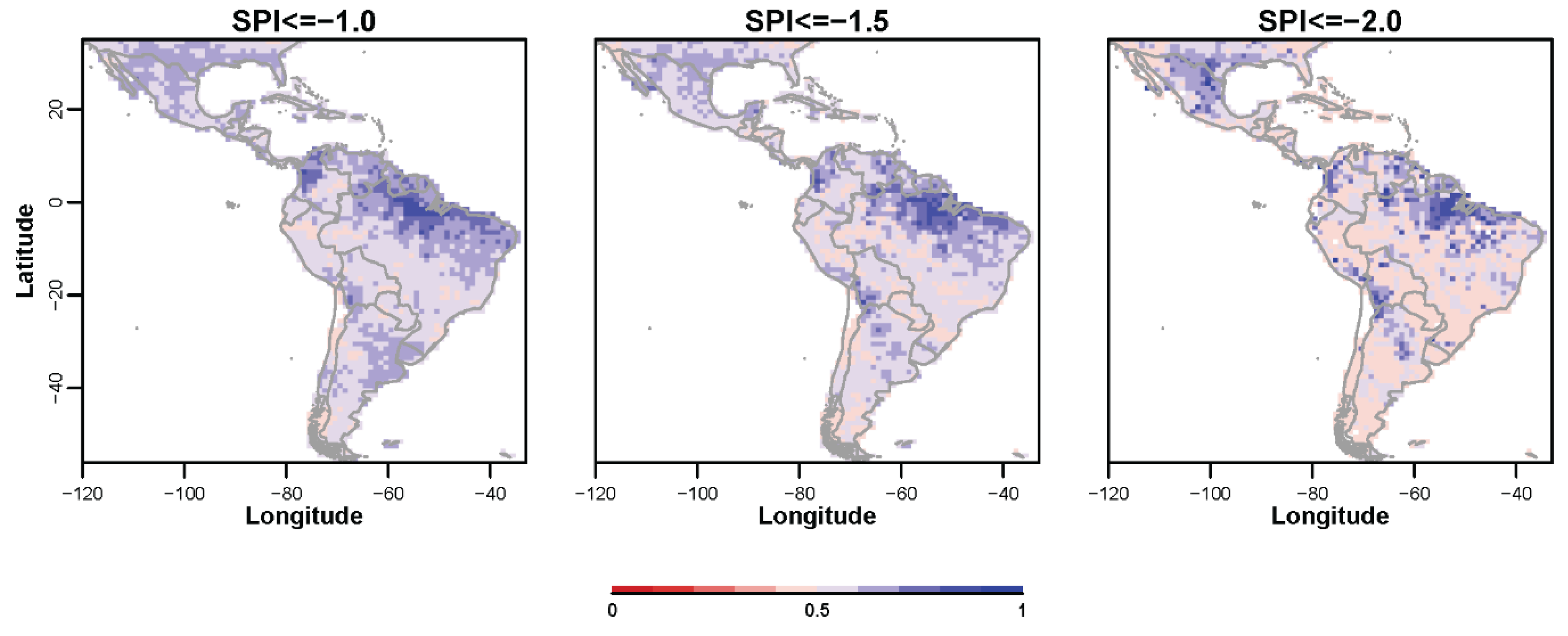
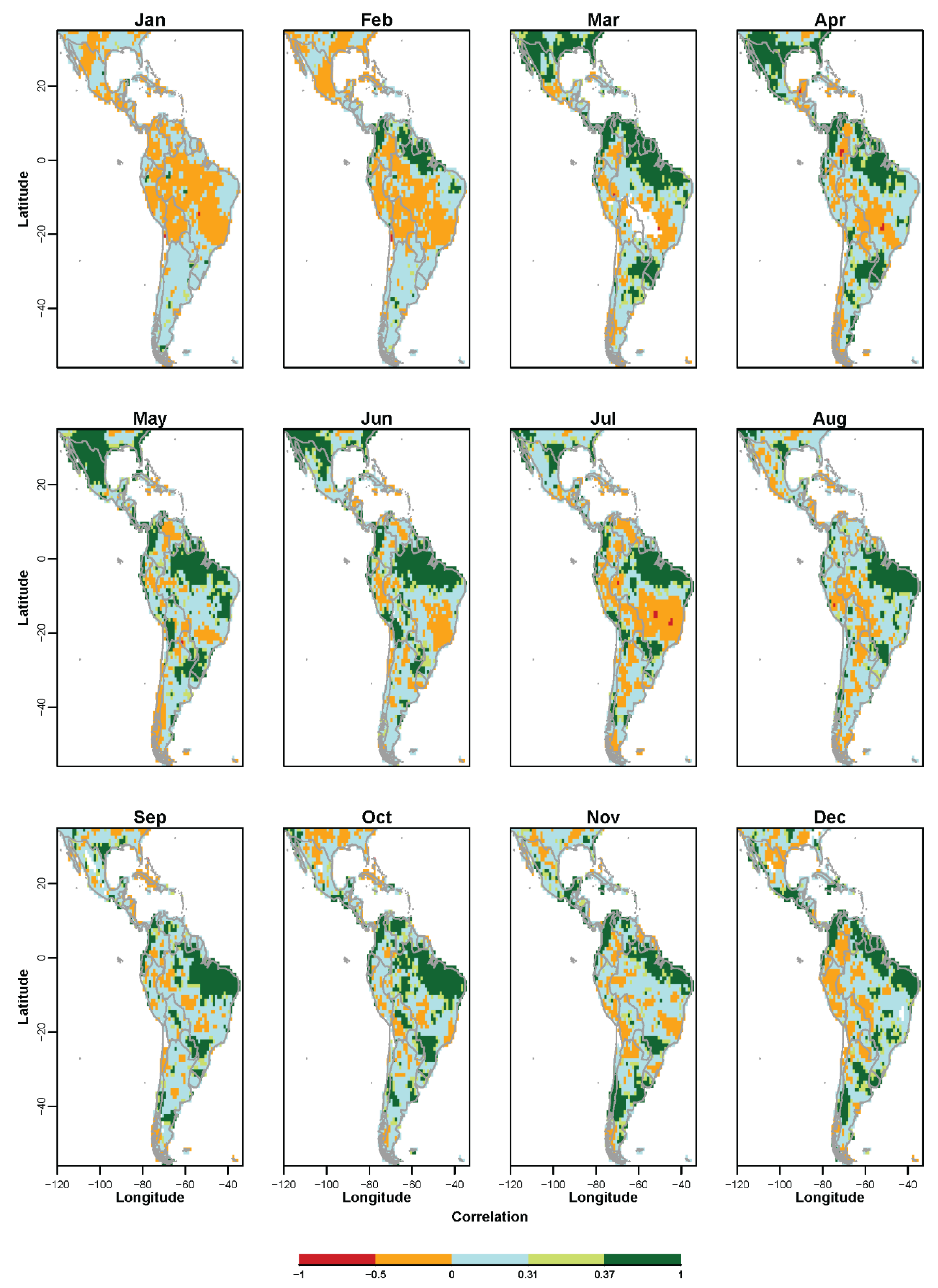
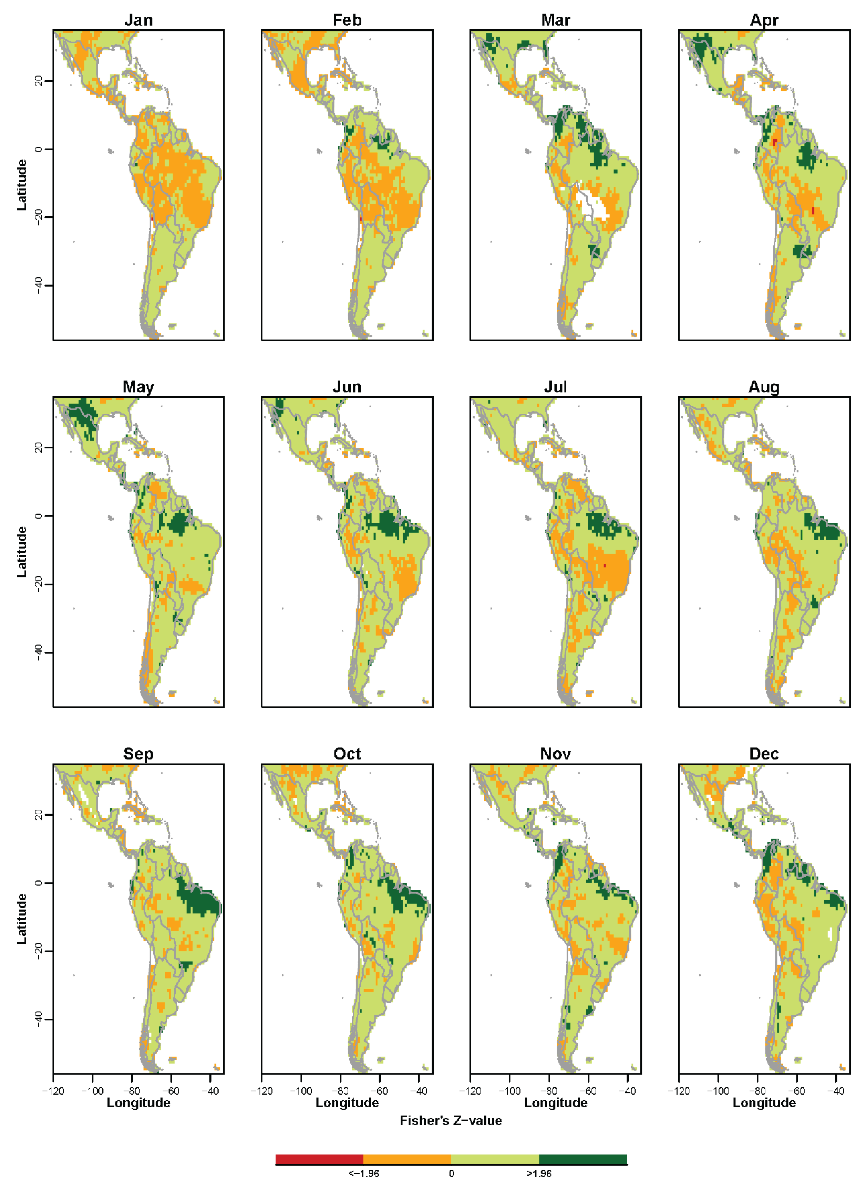
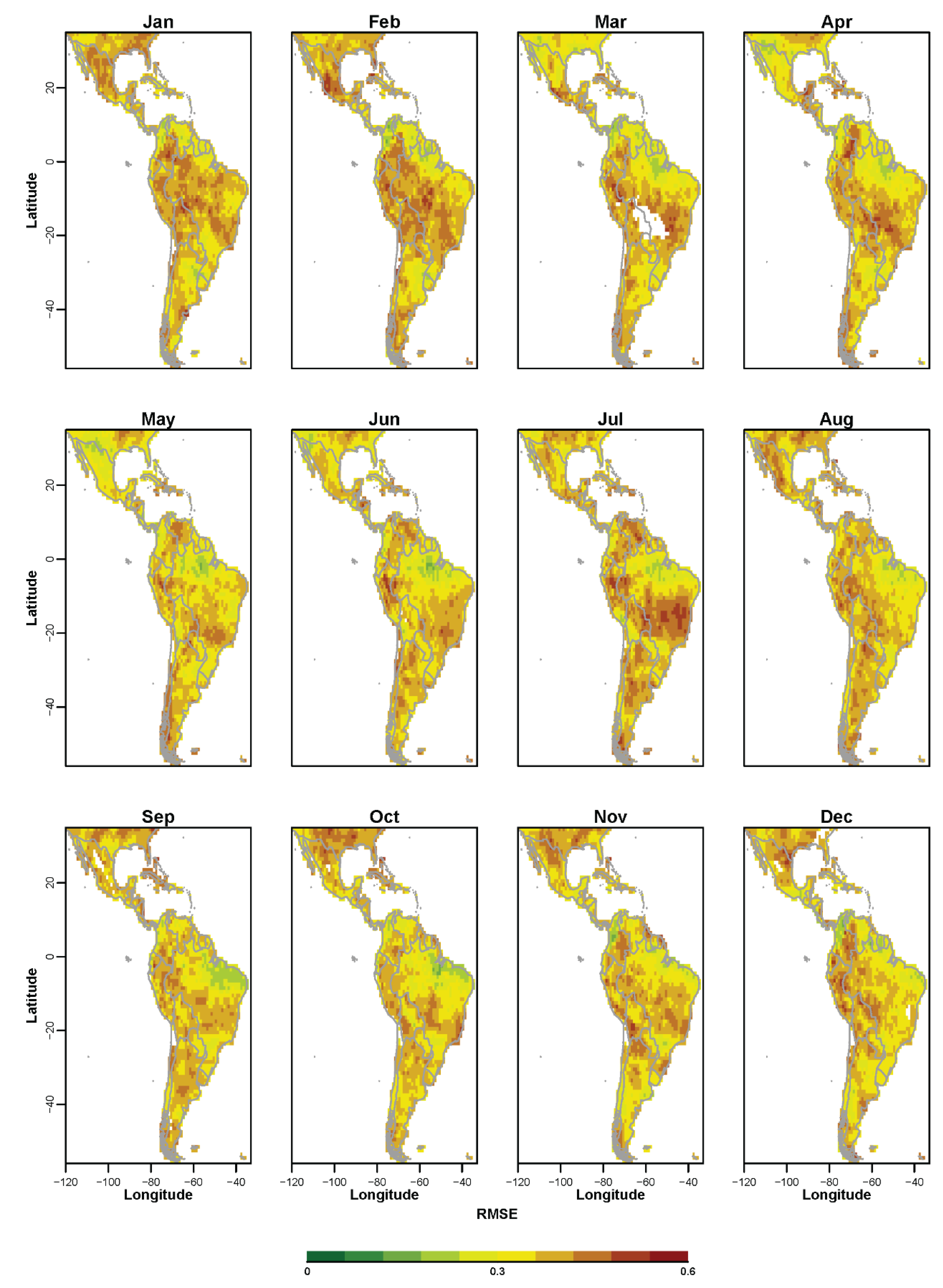
3. Results and Discussion

Initially, we assessed the ability of the ECMWF S4 ensemble system to seasonally forecast the spatial distribution of SPI in South-Central America by evaluating its monthly scalar accuracy and skill score at each location with 3- and 6-month lead time (respectively for the SPI3 and SPI6). In the sequence, we verify the non-probabilistic identification of drought events by means of the S4 system.

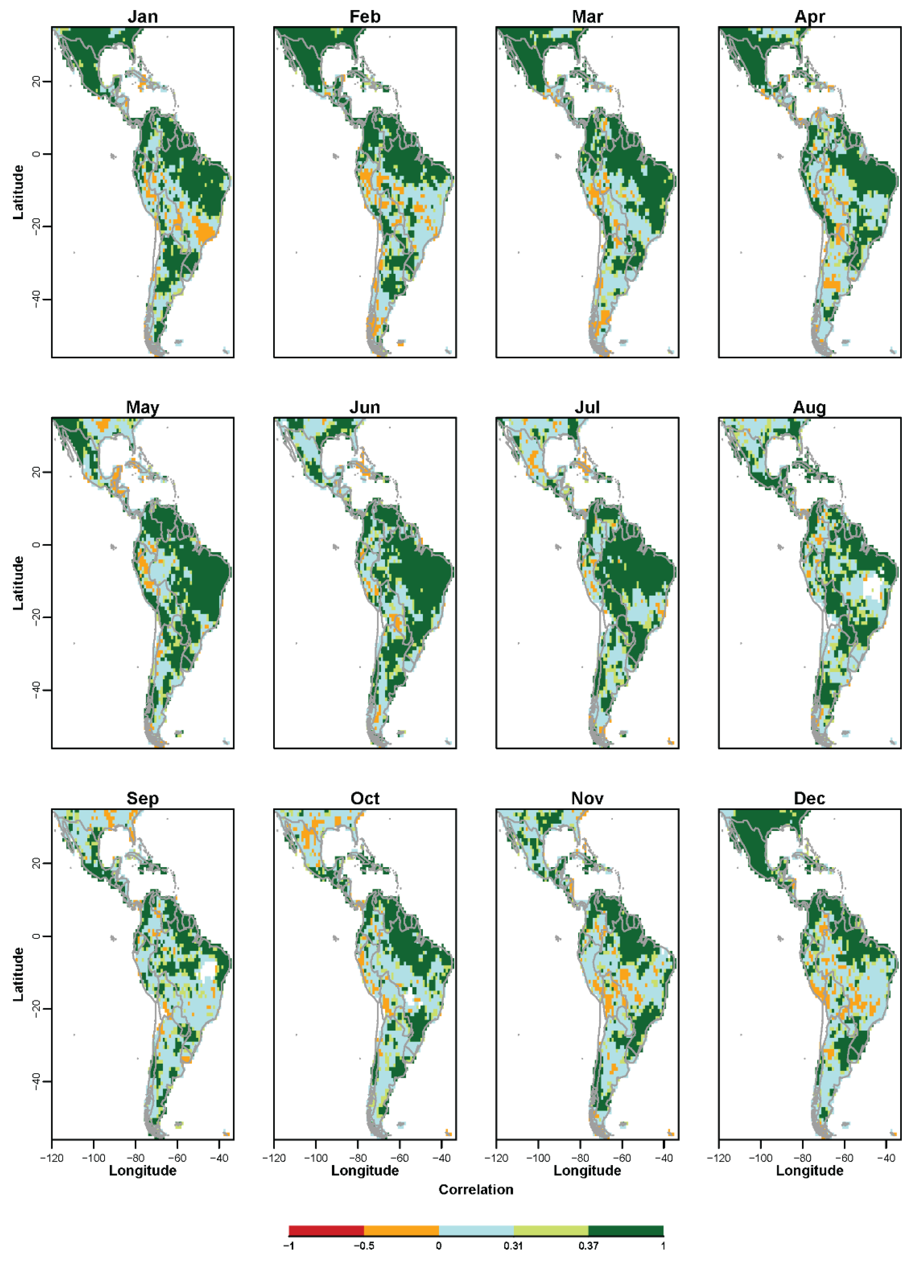
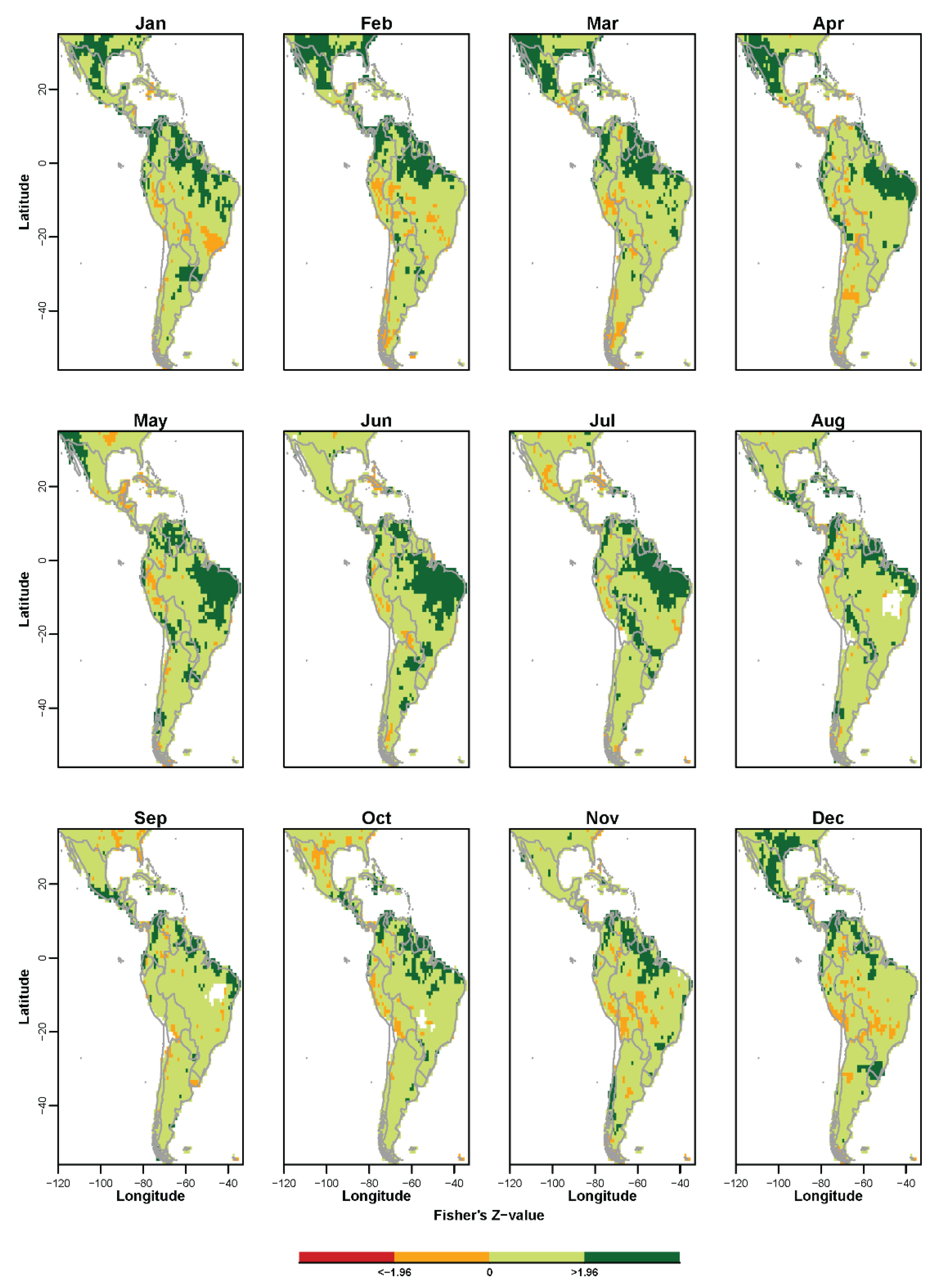
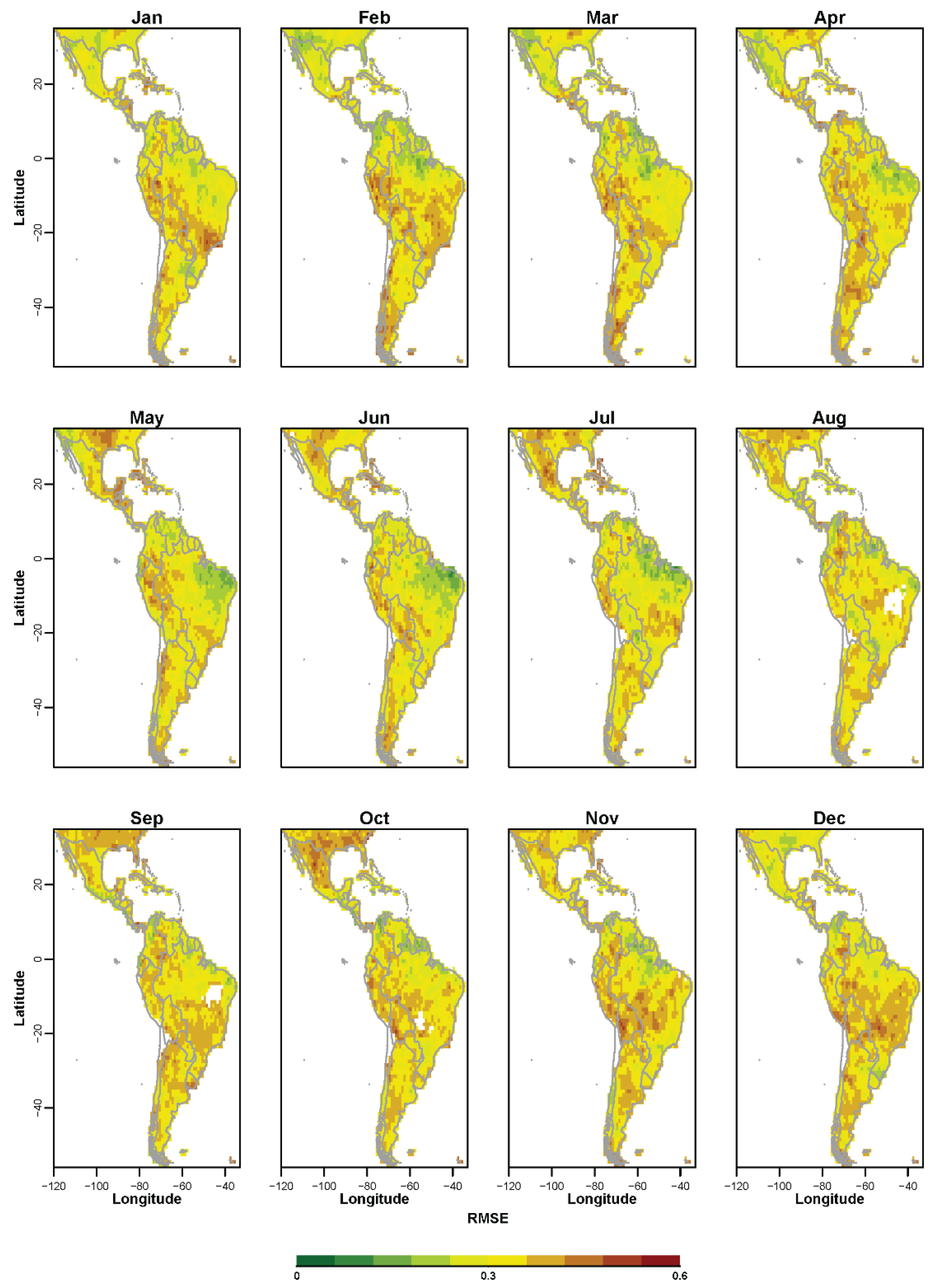
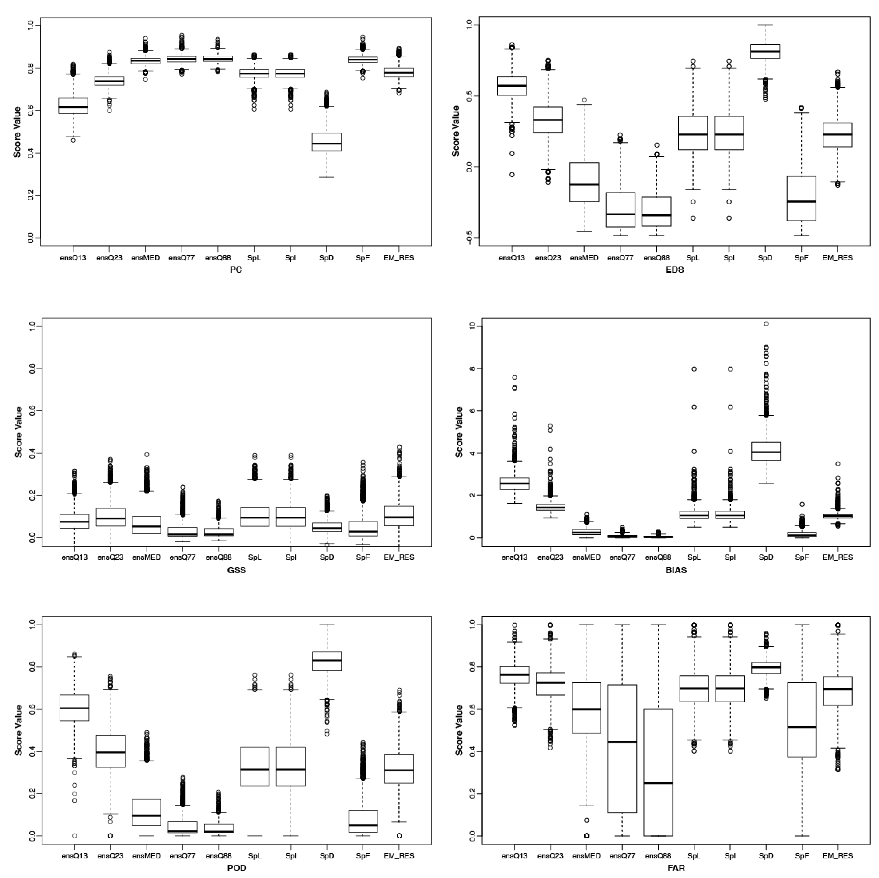
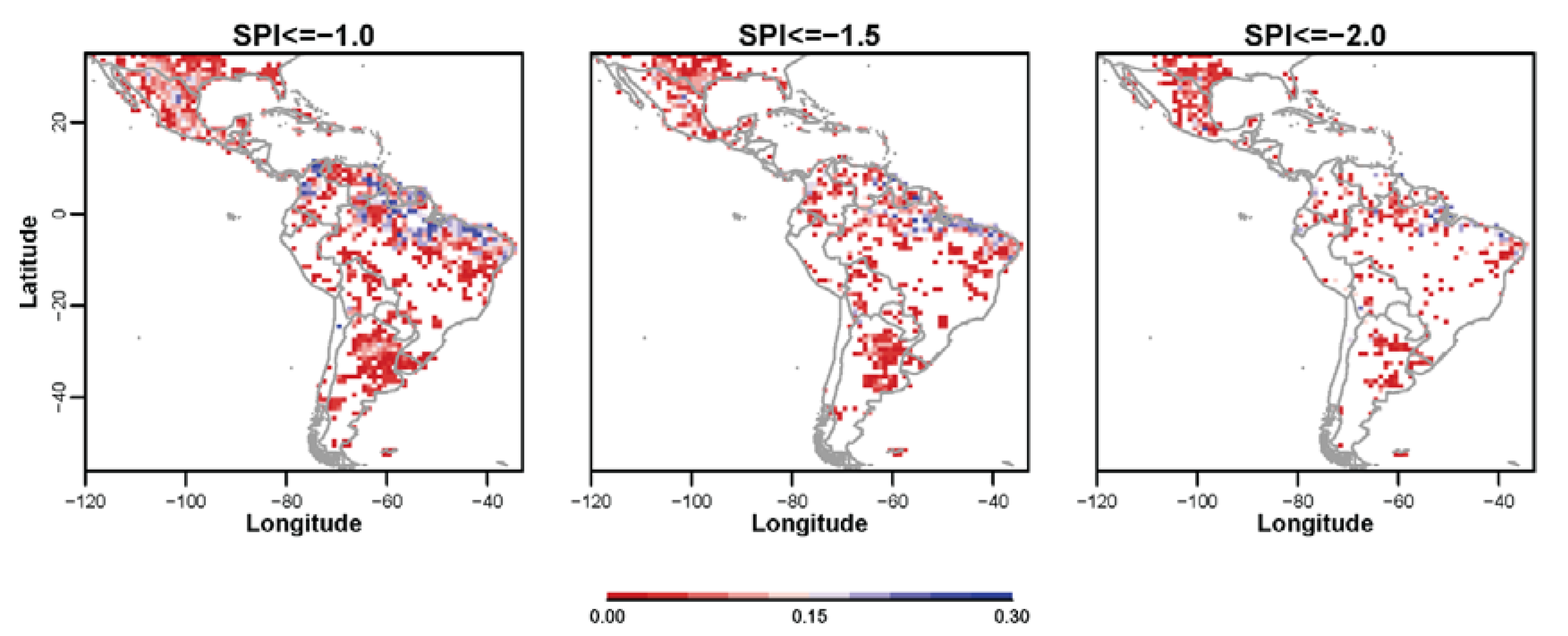
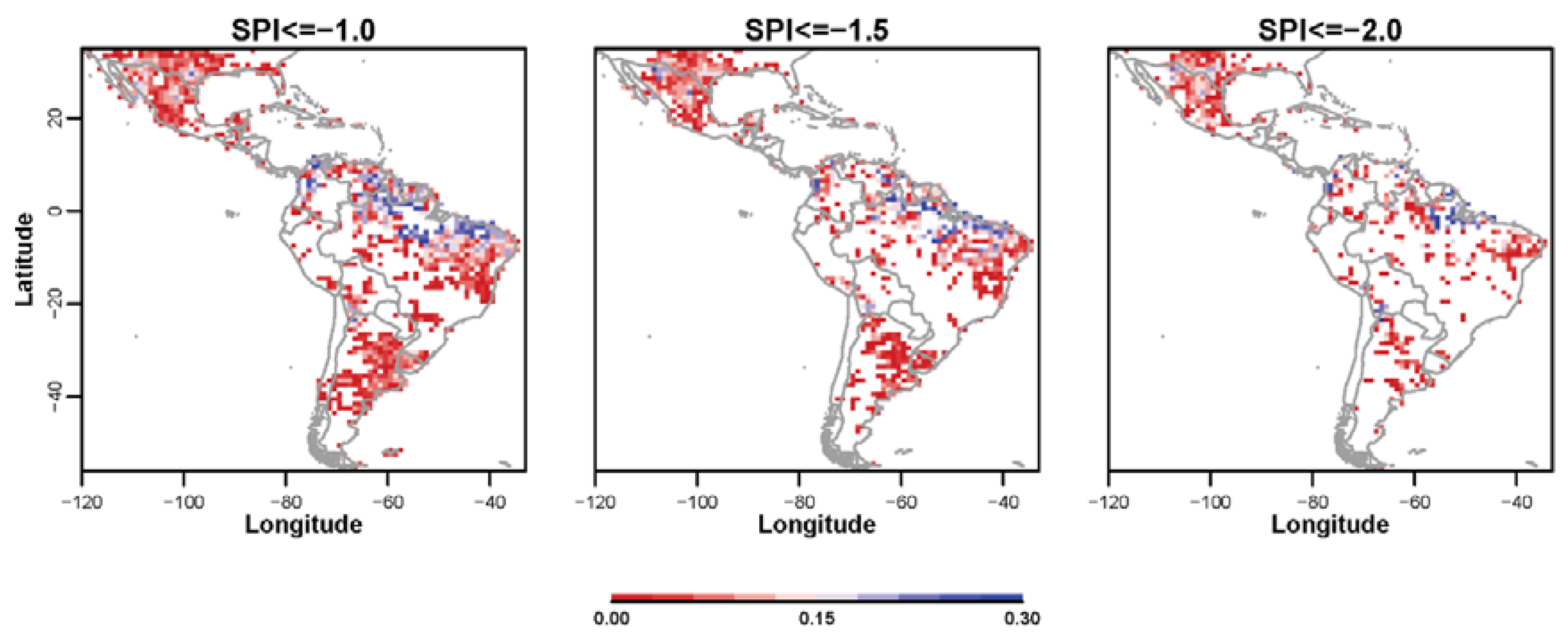
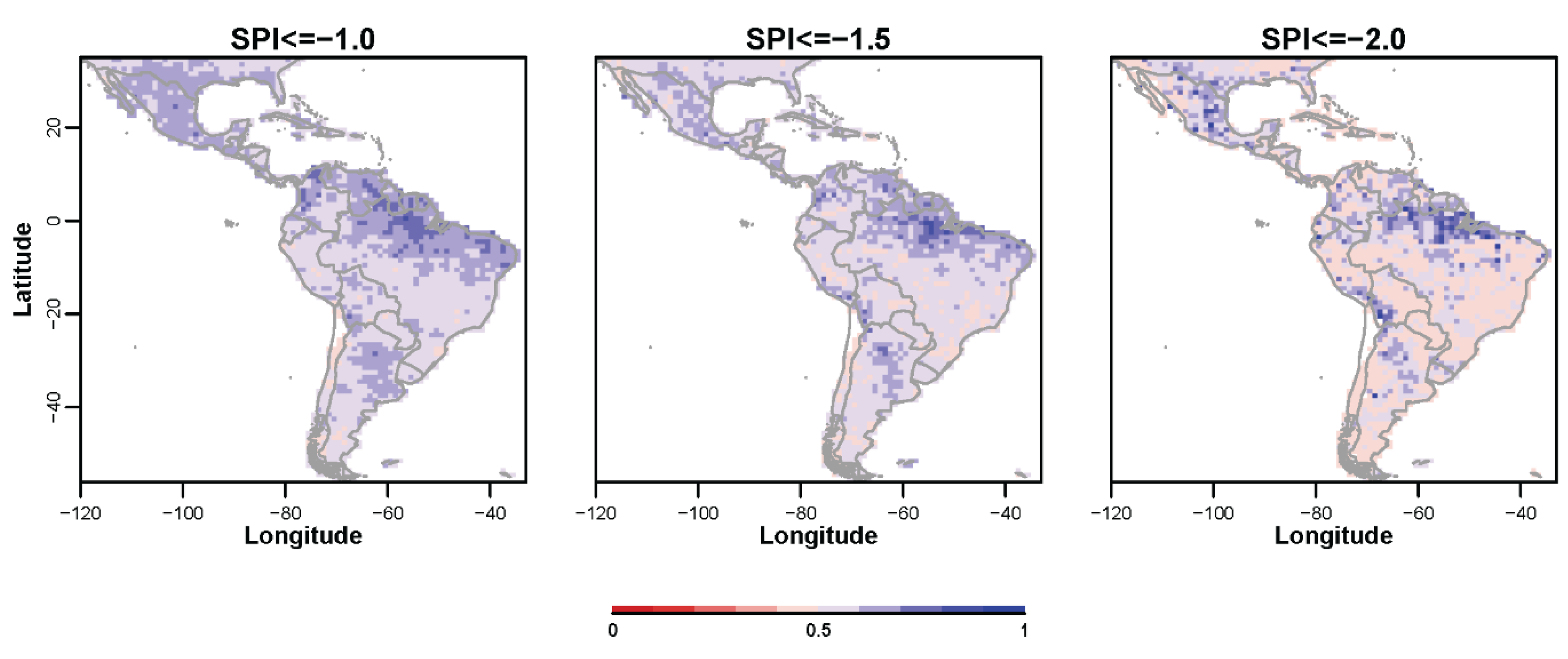
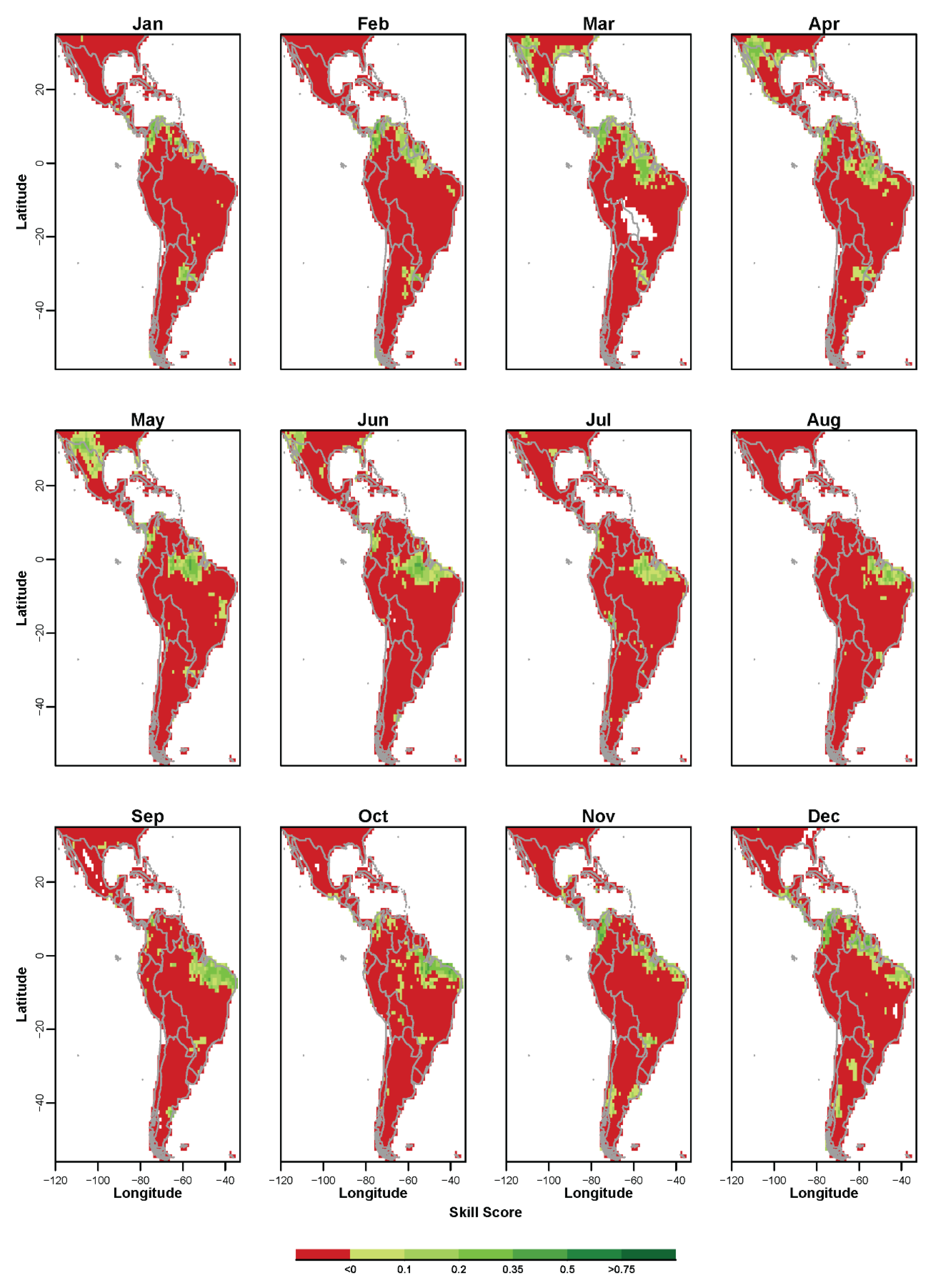
3.1. Non-Probabilistic Forecasts of Continuous SPI Values

In Figure 1, we present the monthly correlation between observed and forecast ensemble mean (a) SPI3 and (b) SPI6 at, respectively, 3- and 6-month lead time for the hindcast period of 1981–2010. The maps depicted in Figure 1 show that there is a positive correlation between SPI3 forecast and observations at all months and for most of the study area. Overall, the forecast SPI3 values follow the trends (increases or decreases) of the observed SPI3 values. Notwithstanding, the statistical significance between observed and forecast SPI3 varies across regions and months: for example, the correlation along the East Pacific coast is almost never statistical significant during the year, it is mostly statistical significant during the whole year for Northeast of South-America, and significant patterns are only verified for Central America during the months between December and May. On the other hand, SPI6 forecasts present extensive geographic areas that are negatively correlated with SPI6 observations at 6-month lead time (Figure A1). These large forecast errors are not systematic but occur mainly for the Amazon and Central East part of South America, and are most evident during the months of January–April (end of the wet season) and June–August (dry season). Surprisingly, and similarly to the SPI3, the correlation is statistically significant during almost the whole year for the Northeast of South America and for large parts of Central America from March to May. Mo and Lyon [41] suggest that the statistically significant correlation patterns in Central America and Northeast of South America are likely contributed by the ENSO: these regions are known to have a strong ENSO signal, and the seasonal skillful of precipitation forecasts contribute to the SPI3 and SPI6 seasonal forecasts. Moreover, in those areas and during both seasons (wet and dry), the intra-seasonal patterns of precipitation seem to be highly influenced by the activity of the Madden–Julian Oscillation [42]. Since the correlation is statistical significant for some regions at some months, then it suggests that the forecast has some skill at 3- and 6-months lead time.
The scalar skill score was also analyzed to assess the ability of the forecasts to improve SPI prediction over the climatological median values (i.e., SPI = 0). The differences between the ECMWF-based forecasts and the climatological forecasts (CLM) will indicate whether there is additional skill obtained from the dynamical model forecasts. In Figure 2, we present the monthly SPI3 forecast skill (using the mean of the ensemble) at 3-month lead time relative to baseline skill for the hindcast period 1981–2010, which shows the difference in correlation between the ECMWF S4 SPI3 forecasts and the baseline SPI3 forecasts based on climatological probabilities. Our results confirm that the forecasts have higher skill than the baseline, but the differences are often not significant at the 5% level based on the Fishers Z test. Indeed, although the correlation with observations is extensively significant over the study area, it does not extensively improve over the climatological SPI values. Marked improvements are observed for Northeast Brazil during the months of April–July, Mexico during the months of December–April, and North of South America between January–April. Overall, our results are consistent with [19,41], namely, that it is still challenging to improve on SPI forecasts that are based on climatology and persistence.
Interestingly, scalar skill score results suggest that SPI3 forecasts match the observations in dry regions mainly during the beginning of the dry seasons, while at regions with high rainfall variability and/or during the wet seasons the forecasts are usually less skillful. Therefore, we believe that the ECMWF S4 ensemble mean might underestimate monthly rainfall and thus increase the intensity of dry periods and lessen the forecast values of SPI3 for the study region.
On the other hand, the 6-month seasonal forecasts are less skillful than the 3-month forecasts (Figure A2). Indeed, and as expected from the correlation analysis, skill scores for the SPI6 forecasts are generally lower than for SPI3 and almost not statistically significant at the 5% level. In Figure A2, it is perceptible that regions with meaningful SPI6 forecasts are also depicted as skillful for the SPI3. The monthly skill scores clearly show that the meaningful forecasts are concentrated over the eastern Amazon, namely in most of the states of AP (Amapá), PA (Pará) and MA (Maranhão). Molteni et al. [30] states that some important bias reductions were introduced in S4, as compared to S3, particularly in the tropical Atlantic and Indian Oceans, and some improvements over land areas e.g., in East Asia and over the Amazon Basin. It is possible that these improvements over the bias of the ECMWF S4 precipitation forecasts will reduce the residual errors between observed and predicted seasonal SPI values.
In Figure 3, the Root Mean Squared Error (RMSE) values between observed and forecast SPI3 at 3-month lead time (Figure A3 for SPI6), for the hindcast period 1981–2010. The results suggest that the predicted SPI is less consistent with the observations derived from GPCC for those regions placed in the subtropical subsidence zones around 10° and 30° N/S, such as subtropical southeast and central Brazil, Paraguay and Bolivia, as well as large areas of Peru.
The high variability of precipitation regimes within those latitudes [43,44] makes it difficult to predict drought at seasonal scale. The results based on the analysis of residual errors also suggest that locations with monthly forecast errors inferior to 0.2 have significant skill, whereas those superior to 0.5 have negative correlation and are unskillful. This output is confirmed by the monthly skill score measured in terms of the RMSE (Figure 4). The RMSE skill score approximates the skill score computed with the correlation index (Figure 2) and its spatial patterns: overall, seasonal SPI3 and SPI6 forecasts are monthly skillful for a small region in the eastern part of the Amazon Basin.

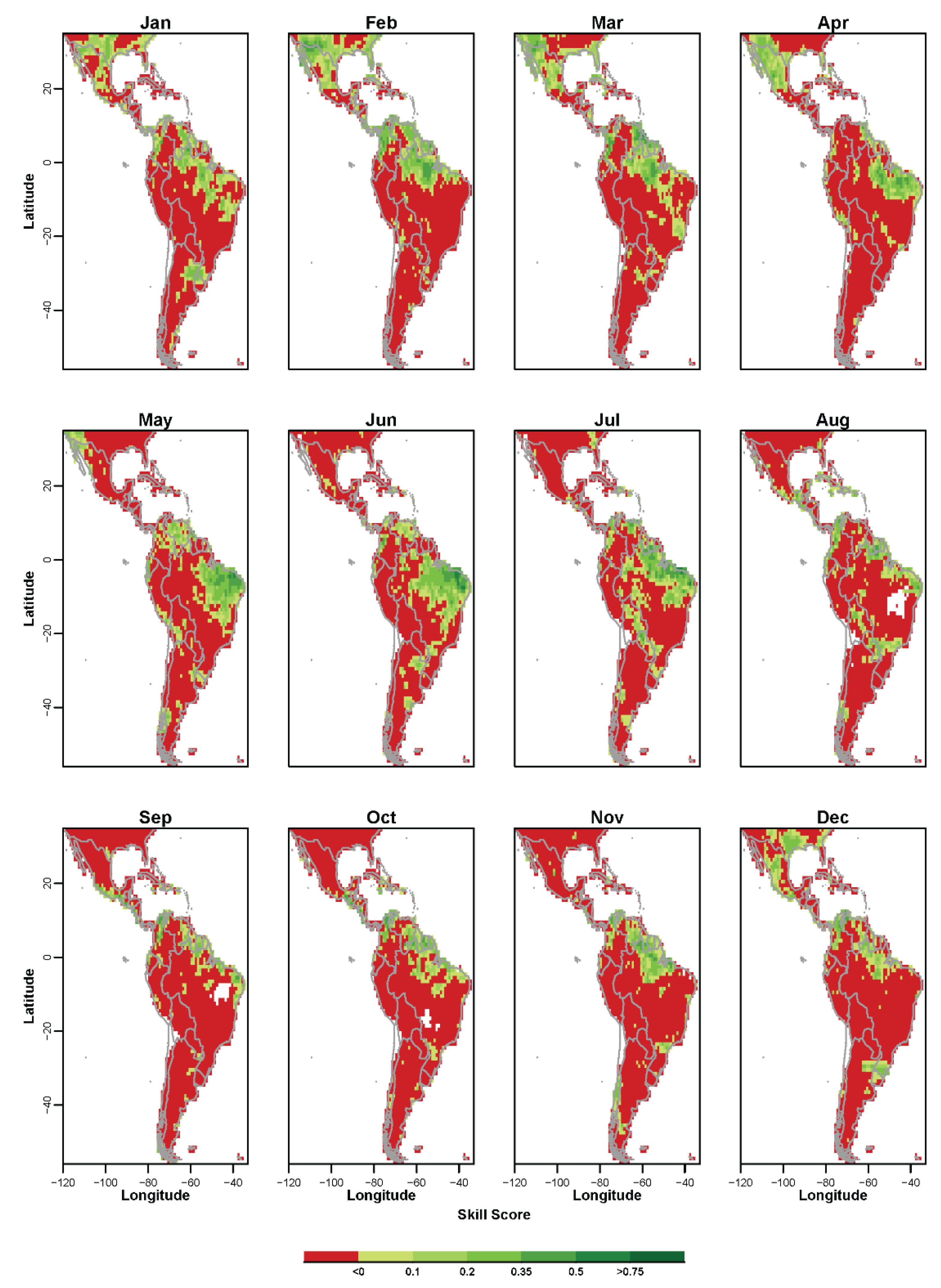
3.2. Non-Probabilistic Forecasts of Categorical SPI Values

In Figure 5 and Figure A5 the score values of categorical drought forecasts are represented (i.e., below the SPI -1 threshold) while the ensemble drought detection was based on several methods as depicted in Table A2. We have pooled together all seasons and locations at the study area in generating Figure 5 and Figure A5. Surprisingly, the distribution of score values for SPI3 and SPI6 are alike for all methods and all verification measures. This may be due to the fact that boundary conditions of seasonal dynamical model forecasts are often characterized by low frequency variability, leading to similar predictability of medium-range climate conditions that extend from a few to several months lead time. In general, precipitation is the result of a complex and interacting phenomena at different spatial and temporal scales, but regional atmospheric patterns that are actively involved in the development of long-term drought conditions are persistent and influenced by predictors that can be accurately estimated at large lead times. Therefore, precipitation anomalies over extreme peak thresholds (drought conditions) might be similarly predicted for different accumulation periods and seasonal lead times, although the accuracy of their scalar values may vary regionally and seasonally. Moreover, given the similar distribution of score values for different methods of categorical drought identification, we present the results of the SPI3 and SPI6 in a joint analysis.
For categorical drought events predicted with both SPI3 and SPI6, computed with the ECMWF S4 ensemble mean (EM-RES), POD values indicate that for at least 50% of the locations in South-Central America one in three seasonal drought events is correctly predicted. This is better than the respective climatology (16% of drought events are correctly detected) and extends over a geographic area larger than that with statistical significant scalar skill scores. Although the ensemble mean performs better than the climatology, POD values are still higher for the methods Q13 (60% of detection) and SpD (80% of detection); the worst results of all the methods are given by the wettest members of the ranked distributions (Q77 and Q88). This means that drier members are better than the mean at detecting the drought onset, but also that there is a low consistency between the extreme and dry members of the ECMWF S4 ensemble set. Lavaysse et al. [40] found similar results in in Europe, where the highest POD is achieved by using the 13 percentile, and the product using the Q13 and Q23 (SpD).
According to the FAR scores, we perceive that by using the ensemble mean SPI values to correctly detect a drought (EM_RES), there will be on average a 70% rate of false alarms. Median FAR values are even larger for dryer members (10% more for Q13 and SpD), and the inter-quantile range of the wettest members is about six times greater than that of the mean (60%), which indicates a large spread of FAR values. Based on these results, it is difficult to select the method that better optimizes between the number of drought hits and the number of misses. Indeed, while the mean of the ensemble shows always an average number of hits and misses (as similar to Spl and SpL, which represent the mean of ensemble extreme and opposite members), the dryer and wetter members of the ensemble attain, respectively, extreme numbers of hits or misses. In that sense, Lavaysse et al. [40] proposed a way to compensate the effect of number of event detected in POD and FAR by using specific thresholds in order to select the same number of events for the different methods.
Looking at PC, we might suggest that the Q13 of the ensemble is the worst performing method to detect between drought and non-drought events. On the other hand, by looking the EDS we might suggest that Q13 is the best method to detect the onset and end of a drought. Because of the non-dependency of the EDS alone to assess a model’s performance on size is fixed, Ghelli and Primo [45] have suggested to not use the EDS alone to assess a model’s performance on forecasting rare events. Those authors have shown that the EDS equation results in an increased freedom of false alarms and correct negatives, which can freely vary with the only restriction that their sum has to be constant. This feature encourages hedging, that is, forecasting the event all the time to guarantee a hit and thus to ensure a higher success rate, however this will increase the false alarm ratio and bias. Therefore, it is paramount to use the EDS in combination with other scores that include the right hand side of the contingency table, as the false alarm rate and/or the bias. Indeed, both FAR and BIAS show that SpD is not an accurate method to detect drought, as it forecasts a large number of drought events that do not occur.
In that sense [40] proposes the use of the maximum Gilbert skill score (GSS) as trigger-point to find the method that better optimizes among the number of false alarms, misses and hits of drought events identified with the SPI. Looking at Figure 5 and Figure A5, it is noted that the ensemble mean (EM_RES) is the best choice for discriminating among seasonal drought and non-droughts events at 3- and 6-month lead time, whilst keeping a minor number of false alarms. Although the SpD gives the best POD, it also increases the ratio of false alarms and diminishes the overall skill score of the method. Following the approach by [40], we suggest that the ensemble mean should be used to trigger the warning of seasonal drought events for South-Central America by means of the SPI3 and SPI6 for respectively 3- and 6-month lead times.

3.3. Probabilistic Forecasts of Categorical SPI Values

In addition to having skillful forecasts of scalar SPI3 and SPI6 derived with the ECMWF S4 ensemble mean at seasonal lead times, a second fundamental challenge to generate reliable drought forecasts for the region is associated with uncertainties in the ensemble used. Therefore, to further quantify the uncertainties arising from the spread of the ensemble when computing the SPI, we computed the overall Brier Skill Score (BSS), based on the climatological frequency of “moderate”, “severe” and “extreme” drought events (Table A1). In Figure 6 and Figure 7, we map the spatial distribution of BSS for the ECMWF S4 SPI-3 and SPI6 forecast respectively, measured in terms of the BS relative to climatological BS at a lead time of 3 and 6 months for the hindcast period 1981–2010. We have pooled together all seasons at each grid point.
The spatial distribution of BSS suggest that the skill of the forecasting system is very similar for both accumulation periods and decreases with the increasing intensity of drought. Looking at the skill for predicting “moderate” drought events, the maps introduced in Figure 6 and Figure 7 show that the forecasting system behaves better than the climatology for large clustered points at the North of South America, Mexico, Northeast of Argentina and Uruguay. In the later regions, where a hot spot appears over La Plata basin, local feedbacks between soil properties and precipitation variability can explain the improved skill which is linked to the coupling strength between soil moisture, evapotranspiration, and temperature [46,47]. On the other hand, the system skill for predicting “extreme” drought events is limited to a few locations in Northeast Brazil, Northeast Mexico, Northeast Amazon, and Northeast of Argentina. These results are encouraging, but only the Northeast of Mexico shows some spatial clustering with positive BSS for extreme drought events, while positive BSS is spatially scattered for the other regions. On combining these results, it can thus be reasonably assumed that forecasting different magnitudes of meteorological drought intensity on seasonal time scales remains quite challenging, but the ECMWF S4 forecasting system does at least a promising job in capturing the drought events (i.e., “moderate” drought) for some regions.
It is interesting to note that the spatial pattern of positive BSS at different SPI categories closely matches the regions that show significant skill scores for non-probabilistic drought forecasts, as well as the geographic grid points that have the lowest monthly RMSEs (Figure 3). As expected, the BSS is lower for the locations where the scalar mismatch between the forecast and observations is larger, which implies more categorical misses and/or false alarms at any SPI intensity. Notwithstanding, since the increase of SPI intensity is accompanied by a decrease of the respective cumulative probability, it was expected that the BSS would decrease with an increase of the SPI drought category because there is a larger probability for mismatching.
To finalize the evaluation of seasonal drought forecasts with the ECMWF S4 data set for South-Central America, we proceed with the analysis of the Relative Operating Characteristic (ROC) of the forecasts. In Figure 8 and Figure 9, we present the spatial distribution of the area under the ROC curve for the probability of drought detection at different SPI frequencies. The values are estimated considering the ECMWF S4 SPI3 and SPI6 forecasts at a lead time of 3 and 6 months respectively, for the hindcast period. We have pooled together all seasons at each 1dd grid point in generating the maps of Figure 8 and Figure 9. For the SPI3 and SPI6, for the “moderate” drought threshold, the area under the ROC curve at all grid points in South-Central America is well above the no skill line, indicating that, despite the poor reliability measured by the BSS, the forecasting system does have some skill. Nevertheless, similarly to the BSS, we perceive that the regions in the North of South America, Northeast of Argentina and Mexico are more skillful than the remaining locations. As the intensity of drought increases, the usefulness of the forecasting system decreases both in magnitude and area. For “extreme” drought events, the grid-points located in South, Central and Northeast of South America are not skillful, as the area under ROC curve is below the 0.5.

4. Conclusions

Here we present and assessment of seasonal drought forecasts, as characterized by the SPI at 3- and 6-months accumulation periods for, 3- and 6-month lead times, respectively. The main advantage of using the SPI for drought monitoring and prediction is that it is already used in operational monitoring systems in many countries around the globe and it is the drought index endorsed by the World Meteorological Organization (WMO).
We evaluated the scalar accuracy of the SPI forecasts together with the skill of probabilistic forecasts of discrete drought events (i.e., <−1). The skill of probabilistic drought identification with the SPI was also assessed. The scalar skill of the SPI-3 and SPI-6 was found to be seasonally and regionally dependent, but for some locations, SPI3 predictions at a lead of 3 months and SPI6 predictions at a lead of 6 months are found to have “useful” skill (monthly correlation with observations is statistically significant at the 5% significance level). The difference in skill between the ECMWF S4 SPI forecasts for South-Central America and a baseline forecast based on the climatological characteristics is positive in many areas and for many months, however it is mostly statistically insignificant. Nevertheless, for the SPI-3, our results show that the skill of the dynamic seasonal forecast is always equal to or above the climatological forecasts. On the other hand, for the SPI-6, our results indicate that it is more difficult to improve the climatological forecasts.
In a second step, we have evaluated several methods to forecast the drought events from the ensemble. Ensemble drought detection was based on several methods (Table A2) and can be organized into three types [40]: individual, where the index is based on an individual member or percentile; partially integrative, where the sum of particular individual members or percentiles are used; and integrative, which is represented by the ensemble mean. Although individual dry members and partially integrative methods were providing an outstanding accuracy for seasonal drought detection, our results have shown that the spread of the ensemble is too large and these methods also have large bias and false alarm ratio. The best (or most consistent) method is defined by using the ensemble mean SPI values, both for SPI3 and SPI6, at three and six months lead times. Our decision was based on the GSS index, which according to many authors provides an optimum solution for selection a classification method based on the number of hits, misses and false alarm ratio. The ensemble mean achieves an overall accuracy of about 80%, with POD above 30% for at least 75% of the study area, and false alarm ration that is overall below the 70%. Although the ECMWF S4 forecast system often overestimates the drought onset, it is significantly better than using the climatology ( 16%).
Finally, standard verification measures for probabilistic forecasts were used to assess the accuracy of drought predictions based on the SPI values for “moderate”, “severe” and “extreme” categories. The Brier Skill Score, which measures the probabilistic forecast skill against a forecast derived from the climatology, showed that both the SPI3 and SPI6 were, for some regions, slightly more skillful that the climatology. The ECMWF forecast system behaves better than the climatology for clustered grid points at the North of South America, Northeast of Argentina and Mexico. The skillful regions are similar for SPI-3 and -6, but become reduced in extent for the most severe SPI categories. We hypothesize that, because an increase of SPI intensity is accompanied by a decrease of the respective cumulative probability, the likelihood of mismatching is larger. As expected, the BSS is lower for the locations where the scalar mismatch between the forecast and the observations is larger, which implies more categorical misses and/or false alarms at any SPI intensity.
Forecasting different magnitudes of meteorological drought intensity on a seasonal time scale still remains a challenge. However, the ECMWF S4 forecasting system does capture reasonably well the onset of drought events (i.e., “moderate” drought) for some regions and seasons. A match is noticeable between observed and predicted SPI for dry months in arid regions with highly marked precipitation seasonality. Although the performance of Numerical Weather Prediction models is always improving and advances in the representation of physical processes in the models is an area of intense active research, the performance is still not good enough to provide useful guidance on months with high precipitation amounts; but it provides information that is more skillful than the climatology for dry periods.

Author Contributions

Conceptualization, H.C., G.N. and P.B.; Methodology, H.C., G.N. and C.L.; Data computation, H.C. and E.D., Validation, all authors; Writing-Original and Draft Preparation, All authors; Writing-Review & Editing, all authors.

Funding

This research received support from the EUROCLIMA regional cooperation program between the European Union (European Commission; DG DEVCO) and Latin America.

Conflicts of Interest

The authors declare no conflict of interest.

Appendix A. Description of the Validation Metrics

Appendix A.1. Nonprobabilistic Forecasts of Continuous SPI Values

We first verify the scalar accuracy of the SPI values for the multimodel ensemble mean at 3 and 6 months lead time (respectively for SPI3 and SPI6). Ensemble mean SPI values are verified against observations for the hindcast period (i.e., from 1981 to 2010). In this case, the SPI magnitude can take any value in a specified segment of the real line, rather than being limited to a finite number of discrete classes (see Table A1). We perform an independent verification of drought forecasts for each month, by using four common accuracy measures of continuous nonprobabilistic forecasts, namely: the Pearson product-moment correlation coefficient, r; the Mean Error (ME); and the Root Mean Squared Error (RMSE). To be considered statistically significant at the 5% (10%) confidence level, the r between forecast SPI values and those in the verifying GPCC data needs to be greater than 0.37 (0.31), as defined by [41] for Nyears = 29 observations (i.e., after subtracting 1 year from the total number of available years in the dataset).
Although the correlation does reflect linear association between two variables (in this case, forecasts and observations), it is not sensitive to biases that may be present in the forecasts. On the other hand, the ME, which is the difference between the average forecast and average observation, expresses the bias of the forecasts. Forecasts that are, on average, too high will exhibit ME > 0 and forecasts that are, on average, too low will exhibit ME < 0. It is important to note that the bias gives no information about the typical magnitude of individual forecast errors, and is therefore not in itself an accuracy measure. To complement the ME, we have computed the RMSE, which has the same physical dimensions as the forecasts and observations, and can be thought of as a typical mean magnitude for individual forecast errors.
We also verify the skill score for the multimodel ensemble mean at 3 and 6 months lead time (respectively for SPI3 and SPI6). Skill score refers to the relative accuracy of an ensemble set of forecasts and is interpreted as the improvement over a reference forecast [48]. Therefore, if the ECMWF S4 is providing value-added skill to the SPI forecasts, it will first be manifested by temporal correlations with observations, r1, that exceed the expected correlation of the same observations with the climatological SPI baseline value (0), r2. Under the assumption that the sets of forecasts are normally distributed, to assess the statistical significance of the difference between two correlations r1 and r2, we used Fisher’s Z transformation, as explained in [49]. We define Zi as
Z i = 1 2 ln ( 1 + r i 1 r i )
for i = 1 and 2. The transformation Z is assumed to be normally distributed with variance (N − 3) − 1, where N = 29 observations (i.e., after subtracting 1 year from the total number of available years in the dataset). We then transformed r1 and r2 to Z1 and Z2, and computed the statistical significance for the difference in correlations using the Z statistics:
Z = Z 1 Z 2 1 N 1 3 + 1 N 2 3
where N1 − 3 and N2 − 3 are the degrees of freedom for r1 and r2, respectively. Using a null hypothesis of equal correlation and a non-directional alternative hypothesis of unequal correlation, if Z is greater than 1.96, the difference in correlations is statistically significant at the 5% confidence level.
A complementary skill score measure was constructed using the RMSE as the underlying accuracy statistic. The reference RMSE is based on the climatological average SPI, and is computed as:
R M S E C l i m = 1 N k = 1 N ( S P I ¯ S P I k ) 2
For the SPI, the climatological average does not change from forecast occasion to forecast occasion (i.e., as a function of the yearly index k). This implies that the RMSEClim is an estimate of the sample variance of the predictand. For the RMSE using climatology as the control forecasts, the skill score becomes
S S C l i m = 1 R M S E R M S E C l i m
Because of the arrangement of the skill score, the SSClim based on RMSE is sometimes called the reduction of variance (RV), because the quotient being subtracted is the average squared error (or residual, in the nomenclature of regression) divided by the climatological variance.

Appendix A.2. Nonprobabilistic Forecasts of Categorical SPI Values

The temporal correlation between forecast and observed values of the SPI provides an overall measure of forecast accuracy and skill, one that is not limited to the case of drought alone. Therefore, we also evaluated SPI forecasts in the context of being able to detect drought, that is, when the SPI drops below a particular threshold. Here, we identified a drought event as occurring when the SPI value for a given month was ≤−1, which corresponds to a “moderate drought” category or higher in the classification system presented in Table A1.
Table A1. SPI classification following McKee et al. [8].
SPI ValueClassCumulative ProbabilityProbability of Event [%]
SPI > 2.00Extreme wet0.977–1.0002.3%
1.50 < SPI < 2.00Severe wet0.933–0.9774.4%
1.00 < SPI < 1.50Moderate wet0.841–0.9339.2%
−1.00 < SPI < 1.00Near normal0.159–0.84168.2%
−1.50 < SPI < −1.00Moderate dry0.067–0.1599.2%
−2.00 < SPI < −1.50Severe dry0.023–0.0674.4%
SPI < −2.00Extreme dry0.000–0.0232.3%
Ensemble drought detection was based on several methods (Table A2) and can be categorized into three types [50]: individual, where the index is based on an individual member or percentile; partially integrative, where the sum of particular individual members or percentiles are used; and integrative which is represented by the ensemble mean. The individual types should be seen as providing complementary information about the intensity of the SPI, but also about the distribution of the members. The individual types of drought detection have been subdivided into five classes representing dry members (Q13, Q23), wet ones (Q77, Q88) or the median. The extreme members of the distribution are not used to avoid outliers generally associated with ensemble systems [50].
Table A2. Methods to detect drought events from the S4 ensemble system. Adapted from [40].
NameDefinitionType
13th percentile (Q13)Member located at the 13% of the CDFIndividual
23th percentile (Q23)Member located at the 23% of the CDFIndividual
Median (MED)Member located at the 50% of the CDFIndividual
77th percentile (Q77)Member located at the 77% of the CDFIndividual
88th percentile (Q88)Member located at the 88% of the CDFIndividual
Large spread (SpL)Sum of the extreme members (Q13 + Q88)Partially integrative
Low spread (Spl)Sum of the members (Q23 + Q78)Partially integrative
Dry spread (SpD)Sum of the dry members (Q13 + Q23)Partially integrative
Flood spread (SpF)Sum of the wet members (Q77 + Q88)Partially integrative
Mean (EM_RES)Ensemble meanIntegrative
For 3- and 6-month lead times (respectively for SPI3 and SPI6), we computed several verification measures for the categorical forecasts (i.e., below the SPI “-1” threshold) identified with the methods described in Table A2. All verification measures are based on a contingency table approach, which is applied at each grid point in the study area. The entries in the table are defined as follows: “A” is the number of drought events that are forecast and occur; “B” is the number of drought events that are forecast but do not occur; “C” is the number of drought events that are not forecast but do occur; and “D” is the number of drought events that are not forecast and do not occur. The variable N is the total number of cases analyzed from 1981 to 2010. Based on these values, the percentage correct (PC, perfect = 1) is the ratio of good forecasting events in relation to the total number of events.
P C = A + D N
The extreme dependency score (EDS) provides a skill score in the range [−1, 1] that can be used to find the hit-rate exponent [51]. The EDS takes the value of 1 for perfect forecasts and 0 for random forecasts, and is greater than zero for forecasts that have hit rates that converge slower than those of random forecasts.
E D S = 2 l o g A + B N l o g A N 1
The Gilbert skill score (GSS) measures the fraction of forecast events that were correctly predicted, adjusted for the frequency of hits that would be expected to occur simply by random chance [40].
G S S = A + A * A + B + C A *
where A* is the number of random hits, computed as:
A * = ( A + B ) ( A + C ) N
The GSS is often used in the verification of rainfall forecasts because its “equitability” allows scores to be compared more fairly across different regimes (for example, it is easier to correctly forecast rain occurrence in a wet climate than in a dry climate). However, because it penalizes both misses and false alarms in the same way, it does not distinguish the source of forecast error. Therefore, it should be used in combination with at least one other contingency table statistic, for example, bias. Here, we compute bias as:
B I A S = A + B A + C
The probability of detection (POD, perfect = 1) is the ratio of the total number of observed events that have been forecasted.
P O D = A A + C
The false alarm rate (FAR, perfect = 0) is the fraction of the forecasted events which actually did not occur.
F A R = B A + B

Appendix A.3. Probabilistic Forecast of Categorical SPI Values

Verification of probability forecasts is somewhat more subtle than verification of non-probabilistic forecasts. Since non-probabilistic forecasts contain no expression of uncertainty, it is clear whether an individual forecast is correct or not. On the other hand, unless a probabilistic forecast is either 0.0 or 1.0, the situation is less clear-cut. For probability values between these two (certainty) extremes, a forecast is neither right nor wrong, so that meaningful assessments can only be made using collections of multiple forecast members and observation pairs. A number of accuracy measures for verification of probabilistic forecasts of dichotomous events exist, but by far the most common is the Brier score (BS) [48]. The Brier score is essentially the mean squared error of the probability forecasts, considering that the GPCC drought observation at time k is ok = 1 if a drought event occurs (i.e., SPI ≤ −1), and that the GPCC observation at time k is ok = 0 if a drought event does not occur (i.e., SPI > −1). The BS averages the squared differences between pairs of forecast probabilities, fcstk, and the subsequent binary reference observations,
B S = 1 n k = 1 N ( f c s t k o k ) 2
where the index k again denotes a numbering of the N forecast-event pairs. Comparing the BS with the root-mean squared error, it can be seen that the two are completely analogous. As a mean-squared-error measure of accuracy, the BS is negatively oriented, with perfect forecasts exhibiting BS = 0. Less accurate forecasts receive higher BS values, but since individual forecasts and observations are both bounded by zero and one, the score can take on values only in the range 0 ≤ BS ≤ 1.
Skill scores of the form of SSclim are also often computed for the BS, yielding the Brier Skill Score (BSS):
B S S = 1 B S B S r e f
The BSS is the conventional skill-score form using the BS as the underlying accuracy measure. Usually, for the SPI, the reference forecasts are the relevant climatological probabilities of a drought event taking place with a certain severity (Table A1). For example, the frequency of “Moderate” drought events is approximately the 16%. The BSS ranges between minus infinity and 1; 0 indicates no skill when compared to the reference forecast; the perfect score is 1. A good companion to the BSS is the Relative Operating Characteristic (ROC) of the forecast. ROC is conditioned on the observations, and measures the ability of the probabilistic forecasting system to discriminate between drought events and non-events of different frequencies, that is, the resolution of the forecast. ROC is not sensitive to bias in the forecast (even a biased forecast could give a good ROC). However, the ROC is a measure of potential usefulness of the probabilistic forecast, and the area under the ROC curve gives a measure of its skill. Since ROC curves for perfect forecasts pass through the upper-left corner, the area under a perfect ROC curve includes the entire unit square, so Aperf = 1. Similarly ROC curves for random forecasts lie along the 45° diagonal of the unit square, yielding the area Arand = 0.5. The area A under a ROC curve of interest can also be expressed in standard skill-score form SSROC, as
S S R O C = A 1 / 2 1 1 / 2
Wilks [48] states that SSROC is a reasonably good discriminator among relatively low-quality forecasts, but that relatively good forecasts tend to be characterized by quite similar (near-unit) areas under their ROC curves. The SSROC ranges between 0 and 1; 0.5 indicates no skill, while the perfect score is 1.
Figure A1. Monthly correlation of the observed and forecast SPI at 6-months lead time (SPI6) (using the mean of the ensemble) for the hindcast period (1981–2010). Values are indicated in the color bar: 0.31 (0.37) is statistical significant at 10% (5%) significance level.
Climate 06 00048 g0a1
Figure A2. Monthly difference in forecast skill (Pearson correlation) between the forecast SPI6 at 6-month lead time (using the mean of the ensemble) and climatological SPI for the hindcast period (1981–2010). Values are indicated in the color bar: 1.96 is the statistical significant at the 5% significance level.
Climate 06 00048 g0a2
Figure A3. RMSE between the observed and forecast SPI6 at 6-month lead time (mean of the ensemble) for the hindcast period (1981–2010). Values in difference of percentile magnitude are indicated in the color bar.
Climate 06 00048 g0a3
Figure A4. Skill Score of the SPI6 at 6-month lead time forecast measured in terms of the RMSE relative to climatological RMSE for the hindcast period (1981–2010).
Climate 06 00048 g0a4
Figure A5. Verification measures of categorical drought forecasts (i.e., below the SPI6 “-1” threshold) estimated with the methods described in Table A2.
Climate 06 00048 g0a5

References

  1. Carrão, H.; Singleton, A.; Naumann, G.; Barbosa, P.; Vogt, J. An optimized system for the classification of meteorological drought intensity with applications in frequency analysis. J. Appl. Meteorol. Climatol. 2014, 53, 1943–1960. [Google Scholar] [CrossRef]
  2. Goddard, S.; Harms, S.K.; Reichenbach, S.E.; Tadesse, T.; Waltman, W.J. Geospatial decision support for drought risk management. Commun. ACM 2003, 46, 35–37. [Google Scholar] [CrossRef]
  3. Dai, A. Drought under global Warming: A review. Wiley Interdiscip. Rev. Clim. Chang. 2011, 2, 45–65. [Google Scholar] [CrossRef]
  4. Lloyd-Hughes, B. The impracticality of a universal drought definition. Theor. Appl. Climatol. 2014, 117, 607–611. [Google Scholar] [CrossRef]
  5. Steinemann, A.C.; Cavalcanti, L.F. Developing multiple indicators and triggers for drought plans. J. Water Res. Plan. Manag. 2006, 132, 164–174. [Google Scholar] [CrossRef]
  6. Heim, R.R. A review of twentieth-century drought indices used in the United States. Bull. Am. Meteorol. Soc. 2002, 83, 1149–1165. [Google Scholar] [CrossRef]
  7. Vicente-Serrano, S.M.; Beguerıa, S.; Lopez-Moreno, J.I. A multiscalar drought index sensitive to global warming: The standardized precipitation evapotranspiration index. J. Clim. 2010, 23, 1696–1718. [Google Scholar] [CrossRef]
  8. McKee, T.B.; Doeskin, N.J.; Kleist, J. The relationship of drought frequency and duration to time scales. In Proceedings of the 8th Conference on Applied Climatology, American Meteorological Society, Anaheim, CA, USA, 17–22 January 1993; pp. 179–184. [Google Scholar]
  9. Svoboda, M.; Hayes, M.; Wood, D. Standardized Precipitation Index User Guide; WMO-No. 1090; World Meteorological Organization (WMO): Geneva, Switzerland, 2012. [Google Scholar]
  10. Mishra, A.K.; Singh, V.P. A review of drought concepts. J. Hydrol. 2010, 391, 202–216. [Google Scholar] [CrossRef]
  11. Kim, T.-W.; Valds, J.B. Nonlinear model for drought forecasting based on a conjunction of wavelet transforms and neural networks. J. Hydrol. Eng. 2003, 8, 319–328. [Google Scholar] [CrossRef]
  12. Mishra, A.K.; Desai, V.R.; Singh, V.P. Drought forecasting using a hybrid stochastic and neural network model. J. Hydrol. Eng. 2007, 12, 626–638. [Google Scholar] [CrossRef]
  13. Mishra, A.K.; Desai, V.R. Drought forecasting using stochastic models. Stoch. Environ. Res. Risk Assess. 2005, 19, 326–339. [Google Scholar] [CrossRef]
  14. Vitart, F.; Buizza, R.; Alonso Balmaseda, M.; Balsamo, G.; Bidlot, J.-R.; Bonet, A.; Fuentes, M.; Hofstadler, A.; Molteni, F.; Palmer, T.N. The new VAREPS-monthly forecasting system: A first step towards seamless prediction. Q. J. R. Meteorol. Soc. 2008, 134, 1789–1799. [Google Scholar] [CrossRef]
  15. Nijssen, B.; Shukla, S.; Lin, C.; Gao, H.; Zhou, T.; Ishottama; Sheffield, J.; Wood, E.F.; Lettenmaier, D.P. A prototype global drought information system based on multiple land surface models. J. Hydrometeorol. 2014, 15, 1661–1676. [Google Scholar] [CrossRef]
  16. Yuan, X.; Wood, E.F. Multimodel seasonal forecasting of global drought onset. Geophys. Res. Lett. 2013, 40, 4900–4905. [Google Scholar] [CrossRef] [Green Version]
  17. Hao, Z.; AghaKouchak, A.; Nakhjiri, N.; Farahmand, A. Global integrated drought monitoring and prediction system. Sci. Data 2014, 1, 140001. [Google Scholar] [CrossRef] [PubMed]
  18. Dutra, E.; Wetterhall, F.; Di Giuseppe, F.; Naumann, G.; Barbosa, P.; Vogt, J.; Pozzi, W.; Pappenberger, F. Global meteorological drought Part 1: Probabilistic monitoring. Hydrol. Earth Syst. Sci. 2014, 18, 2657–2667. [Google Scholar] [CrossRef]
  19. Dutra, E.; Pozzi, W.; Wetterhall, F.; Di Giuseppe, F.; Magnusson, L.; Naumann, G.; Barbosa, P.; Vogt, J.; Pappenberger, F. Global meteorological drought Part 2: Seasonal forecasts. Hydrol. Earth Syst. Sci. 2014, 18, 2669–2678. [Google Scholar] [CrossRef] [Green Version]
  20. Spennemann, P.C.; Rivera, J.A.; Osman, M.; Saulo, A.C.; Penalba, O.C. Assessment of seasonal soil moisture forecasts over Southern South America with emphasis on dry and wet events. J. Hydrometeorol. 2017, 18, 2297–2311. [Google Scholar] [CrossRef]
  21. Sheffield, J.; Andreadis, K.M.; Wood, E.F.; Lettenmaier, D.P. Global and continental drought in the second half of the twentieth century: Severity–area–duration analysis and temporal variability of large-scale events. J. Clim. 2009, 22, 1962–1981. [Google Scholar] [CrossRef]
  22. Zhao, M.; Running, S.W. Drought-induced reduction in global terrestrial net primary production from 2000 through 2009. Science 2010, 329, 940–943. [Google Scholar] [CrossRef] [PubMed]
  23. Vargas, W.M.; Naumann, G.; Minetti, J.L. Dry spells in the river Plata Basin: An approximation of the diagnosis of droughts using daily data. Theor. Appl. Climatol. 2011, 104, 159–173. [Google Scholar] [CrossRef]
  24. Field, C.B.; Barros, V.; Stocker, T.F.; Qin, D.; Dokken, D.J.; Ebi, K.L.; Mastrandrea, M.D.; Mach, K.J.; Plattner, G.-K.; Allen, S.K.; et al. (Eds.) Managing the Risks of Extreme Events and Disasters to Advance Climate Change Adaptation; Cambridge University Press: New York, NY, USA, 2012; pp. 1–19. [Google Scholar]
  25. Penalba, O.C.; Rivera, J.A. Future changes in drought characteristics over Southern South America projected by a CMIP5 multi-model ensemble. Am. J. Clim. Chang. 2013, 2, 173–182. [Google Scholar] [CrossRef]
  26. Trenberth, K.E.; Stepaniak, D. Indices of El Niño evolution. J. Clim. 2011, 14, 1697–1701. [Google Scholar] [CrossRef]
  27. FAO. Aquastat Database. Food and Agriculture Organization of the United Nations (FAO). 2017. Available online: http://www.fao.org/nr/water/aquastat/main/index.stm (accessed on 15 October 2017).
  28. Magrin, G.; Garcia, C.G.; Choque, D.C.; Gimenez, J.C.; Moreno, A.R.; Nagy, G.J.; Nobre, C.; Villamizar, A. Climate change, Impacts, adaptation and vulnerability. In Contribution of Working Group II to the Fourth Assessment Report of the Intergovernmental Panel on Climate Change; Parry, M.L., Canziani, O.F., Palutikof, J.P., van der Linden, P., Hanson, C.E., Eds.; Cambridge University Press: Cambridge, UK, 2007; pp. 581–615. [Google Scholar]
  29. Llano, M.P.; Vargas, W.; Naumann, G. Climate variability in areas of the world with high production of soya beans and Corn: Its relationship to crop yields. Meteorol. Appl. 2012, 19, 385–396. [Google Scholar] [CrossRef]
  30. Molteni, F.; Stockdale, T.; Balmaseda, M.; Balsamo, G.; Buizza, R.; Ferranti, L.; Magnunson, L.; Mogensen, K.; Palmer, T.; Vitart, F. The new ECMWF seasonal forecast system (System 4). In Technical Memorandum No. 656; European Centre for Medium Range Weather Forecasts: Berkshire, UK, 2011. [Google Scholar]
  31. Rudolf, B.; Becker, A.; Schneider, U.; Meyer-Christoffer, A.; Ziese, M. New full data reanalysis version 5 provides high-quality gridded monthly precipitation data. GEWEX News 2011, 21, 4–5. [Google Scholar]
  32. Naumann, G.; Barbosa, P.; Carrão, H.; Singleton, A.; Vogt, J. Monitoring drought conditions and their uncertainties in Africa using TRMM data. J. Appl. Meteorol. Climatol. 2012, 51, 1867–1874. [Google Scholar] [CrossRef]
  33. Svoboda, M.; LeComte, D.; Hayes, M.; Heim, R.; Gleason, K.; Angel, J.; Rippey, B.; Tinker, R.; Palecki, M.; Stooksbury, D.; et al. The drought monitor. Bull. Am. Meteorol. Soc. 2002, 83, 1181–1190. [Google Scholar] [CrossRef]
  34. Steinemann, A. Drought indicators and Triggers: A stochastic approach to evaluation. JAWRA 2003, 39, 1217–1233. [Google Scholar] [CrossRef]
  35. Hayes, M.J.; Svoboda, M.D.; Wilhite, D.A.; Vanyarkho, O.V. Monitoring the 1996 drought using the standardized precipitation index. Bull. Am. Meteorol. Soc. 1999, 80, 429–438. [Google Scholar] [CrossRef]
  36. Wu, H.; Hayes, M.J.; Wilhite, D.A.; Svoboda, M.D. The effect of the length of record on the standardized precipitation index calculation. Int. J. Climatol. 2005, 25, 505–520. [Google Scholar] [CrossRef] [Green Version]
  37. Sepulcre-Canto, G.; Horion, S.; Singleton, A.; Carrão, H.; Vogt, J. Development of a combined drought indicator to detect agricultural drought in Europe. Earth Syst. Sci. 2012, 12, 3519–3531. [Google Scholar] [CrossRef]
  38. Ntale, H.K.; Gan, T.Y. Drought indices and their application to east Africa. Int. J. Climatol. 2003, 23, 1335–1357. [Google Scholar] [CrossRef]
  39. Hofer, B.; Carrao, H.; Mcinerney, D. Multi-disciplinary forest fire danger assessment in Europe: The potential to integrate long-term drought information. IJSDIR 2012, 7, 300–322. [Google Scholar]
  40. Lavaysse, C.; Vogt, J.; Pappenberger, F. Early warning of drought in Europe using the monthly ensemble system from ECMWF. Hydrol. Earth Syst. Sci. 2015, 19, 3273–3286. [Google Scholar] [CrossRef] [Green Version]
  41. Mo, K.C.; Lyon, B. Global meteorological drought prediction using the North American multi-model ensemble. J. Hydrometeorol. 2015, 16, 1409–1424. [Google Scholar] [CrossRef]
  42. Vera, C.S.; Alvarez, M.S.; Gonzalez, P.L.; Liebmann, B.; Kiladis, G.N. Seasonal cycle of precipitation variability in South America on intraseasonal timescales. Clim. Dyn. 2017, 1–11. [Google Scholar] [CrossRef]
  43. González, P.L.; Vera, C.S. Summer precipitation variability over South America on long and short intraseasonal timescales. Clim. Dyn. 2014, 43, 1993–2007. [Google Scholar] [CrossRef]
  44. González, P.L.; Vera, C.S.; Liebmann, B.; Kiladis, G. Intraseasonal variability in subtropical South America as depicted by precipitation data. Clim. Dyn. 2008, 30, 727–744. [Google Scholar] [CrossRef]
  45. Ghelli, A.; Primo, C. On the use of the extreme dependency score to investigate the performance of an NWP model for rare events. Meteorol. Appl. 2009, 16, 537–544. [Google Scholar] [CrossRef] [Green Version]
  46. Ruscica, R.C.; Sörensson, A.A.; Menéndez, C.G. Pathways between soil moisture and precipitation in southeastern South America. Atmos. Sci. Lett. 2015, 16, 267–272. [Google Scholar] [CrossRef] [Green Version]
  47. Spennemann, P.C.; Saulo, A.C. An estimation of the land–atmosphere coupling strength in South America using the Global Land Data Assimilation System. Int. J. Climatol. 2015, 35, 4151–4166. [Google Scholar] [CrossRef]
  48. Wilks, D.S. Statistical Methods in the Atmospheric Sciences, 2nd ed.; Academic Press: Amsterdam, The Netherlands, 2005. [Google Scholar]
  49. Quan, X.W.; Hoerling, M.P.; Lyon, B.; Kumar, A.; Bell, M.A.; Tippett, M.K.; Wang, H. Prospects for dynamical prediction of meteorological drought. J. Appl. Meteorol. Climatol. 2012, 51, 1238–1252. [Google Scholar] [CrossRef]
  50. Lavaysse, C.; Carrera, M.; Blair, S.; Gagnon, N.; Frenette, R.; Charron, M.; Yau, M.K. Impact of surface parameter uncertainties within the Canadian regional ensemble prediction system. Mon. Weather Rev. 2013, 141, 1506–1526. [Google Scholar] [CrossRef]
  51. Stephenson, D.B.; Casati, B.; Ferro, C.A.T.; Wilson, C.A. The extreme dependency Score: A non-vanishing measure for forecasts of rare events. Meteorol. Appl. 2008, 15, 41–50. [Google Scholar] [CrossRef]
Figure 1. Monthly correlation of the observed and forecast standardized precipitation index (SPI) at 3-months lead time (SPI3) (using the mean of the ensemble) for the hindcast period (1981–2010). Values are indicated in the color bar: 0.31 (0.37) is statistical significant at 10% (5%) significance level.
Climate 06 00048 g001
Figure 2. Monthly difference in forecast skill (Pearson correlation) between the forecast SPI3 at 3-month lead time (using the mean of the ensemble) and climatological SPI for the hindcast period (1981–2010). Values are indicated in the color bar: 1.96 is the statistical significance at the 5% significance level.
Climate 06 00048 g002
Figure 3. Root Mean Squared Error (RMSE) between the observed and forecast SPI3 at 3-month lead time (mean of the ensemble) for the hindcast period (1981–2010). Values in difference of percentile magnitude are indicated in the color bar.
Climate 06 00048 g003
Figure 4. Skill Score of the SPI3 at 3-month lead time forecast measured in terms of the RMSE relative to climatological RMSE for the hindcast period (1981–2010).
Climate 06 00048 g004
Figure 5. Verification measures of categorical drought forecasts (i.e., below the SPI3 “-1” threshold) estimated with the methods described in Table A2.
Climate 06 00048 g005
Figure 6. Brier Skill Score (BSS) of the European Centre for Medium Range Weather (ECMWF) S4 SPI-3 forecast for different probabilities of SPI occurrence, at a lead time of 3 months for the hindcast period 1981–2010. Values are indicated in the color bar; land grid points colored in white indicate that the forecasting system is no more skillful than the climatology.
Climate 06 00048 g006
Figure 7. Brier Skill Score (BSS) of the ECMWF S4 SPI-6 forecast for different probabilities of SPI occurrence, at a lead time of 3 months for the hindcast period 1981–2010. Values are indicated in the color bar; land grid points colored in white indicate that the forecasting system is no more skillful than the climatology.
Climate 06 00048 g007
Figure 8. Area under the Relative Operating Characteristic (ROC) curve for the probability of drought detection at different SPI3 frequencies. Values indicated in the color bar are estimated at lead time of 3 months for the hindcast period 1981–2010.
Climate 06 00048 g008
Figure 9. Area under the ROC curve for the probability of drought detection at different SPI6 frequencies. Values indicated in the color bar are estimated at lead time of 6 months for the hindcast period 1981–2010.
Climate 06 00048 g009

