Abstract
Earth’s global surface temperature shows variability on an extended range of temporal scales and satisfies an emergent scaling symmetry. Recent studies indicate that scale invariance is not only a feature of the observed temperature fluctuations, but an inherent property of the temperature response to radiative forcing, and a principle that links the fast and slow climate responses. It provides a bridge between the decadal- and centennial-scale fluctuations in the instrumental temperature record, and the millennial-scale equilibration following perturbations in the radiative balance. In particular, the emergent scale invariance makes it possible to infer equilibrium climate sensitivity (ECS) from the observed relation between radiative forcing and global temperature in the instrumental era. This is verified in ensembles of Earth system models (ESMs), where the inferred values of ECS correlate strongly to estimates from idealized model runs. For the range of forcing data explored in this paper, the method gives best estimates of ECS between 1.8 and 3.7 K, but statistical uncertainties in the best estimates themselves will provide a wider likely range of the ECS.
1. Introduction
The Intergovernmental Panel on Climate Change [1] (IPCC) has estimated the likely range of equilibrium climate sensitivity (ECS) to be between 1.5 and 4.5 K. The ECS, which is widely used in assessments of anthropogenic climate change, is defined as the asymptotic temperature increase following an instantaneous CO doubling. In Earth system models (ESMs), the ECS is generally estimated via the so-called Gregory plots [2], where the response in the top-of-the-atmosphere radiation N is plotted against the global mean surface temperature (GMST) anomaly during the equilibration following an instantaneous doubling or quadrupling of the atmospheric CO concentration. The assumption is that the adjustment in radiation depends linearly on the surface temperature increase,
so that the feedback parameter and the forcing F can be determined via linear regression. The ECS is hence , where is the forcing associated with a CO doubling. The Gregory plots show that the linearity assumption is only approximate, and in particular, there are slow feedbacks in the models that reduce the feedback parameter as the planet warms [3]. A state dependence is also observed in the so-called paleo sensitivity [4,5,6,7]. Nevertheless, the usefulness of ECS and its estimation still relies on the linearity assumption in Equation (1). Satellite observations of the top-of-the-atmosphere radiation are available through the Clouds and the Earth’s Radiant Energy System (CERES), but unfortunately, the data only covers the years 2000-present. The state-of-the-art ECS estimates based on the satellite data gives a wide likely range (in this case a 17–83% confidence interval) of 2.4–4.5 K [8].
A different approach, which can be used when the top-of-the-atmosphere radiation is unknown, is to combine model results with the instrumental temperature record. Recently Cox et al. claimed that ECS can be constrained to a “likely range” (in this paper specified to be the 66% confidence interval) of 2.2 to 3.4 K, with a best estimate of 2.8 K [9]. They propose a metric characterizing the correlation structure of the internal variability of the GMST in both the instrumental temperature record in the period 1880 to 2016 and in the corresponding historical runs in the Coupled Model Intercomparison Project Phases 5 (CMIP5) ensemble. By exploring a so-called emergent relationship between ECS and , they estimate a distribution for the Gregory estimate of ECS conditioned on , and using the law of total probability in conjunction with Bayes Theorem, they obtain a probability density function constrained by the instrumental record. However, it has been demonstrated that their estimated metric depends on the response to the strong anthropogenic forcing in the time period after year 1950, and hence one has to take into account that the historical forcing times series used in different models in the ensemble are not exactly the same [10]. Another problem is that the emergent relationship was derived from an oversimplified one-box stochastic energy balance equation (Equation (7) described in Section 2.1). This model does not take into account the memory effects in the response due to heat exchange between the ocean mixed layer and the deep ocean. Models that do incorporate such memory effects are briefly reviewed in Section 2.2 and Section 2.3.
A method of constraining ECS from the instrumental record that does not draw on a simplified physical model is to include data for historical forcing, with its uncertainties, and to estimate response functions that describe the relationship between global radiative forcing and the observed GMST. If one adopts a hypothesis of a linear and stationary response, then the temperature anomaly can be written as a convolution of the forcing F with a response function :
where the term is the known (deterministic) forcing and represents a white-noise random forcing that gives rise to the internal variability. Equation (2) only assumes linearity and stationarity of the response, and it is only the functional form of that depends on the particular physical modeling of this response. As discussed in Section 2.2, such a linear response can be derived from a multi-layer energy balance model, where the response function is a sum of exponential functions with decay rates that are given by the real and negative eigenvalues of the system of differential equations. Fredriksen and Rypdal [11] have shown that three exponential terms are sufficient to obtain a model that simultaneously displays responses to historical and reconstructed forcing that are consistent with the instrumental temperature record and the reconstructed last millennium global mean temperature, respectively. In addition, it correctly describes the statistical properties of the internal variability on time scales from months to centuries [12]. The constructed response function corresponds to an ECS estimate of 3.0 K, obtained by using the forcing in Equation (2), where is the unit step function. Defining the ECS as , Equation (2) yields
The forcing is well approximated by a logarithmic dependence of the CO concentration, with a best estimate of 3.7 W/m found by the IPCC [1]. Uncertainties associated with the radiative transfer calculations are small [13]. However, forcing estimates from CMIP5 models often include rapid adjustments of the atmosphere, resulting in larger uncertainties [14]. The more serious issues are the uncertainty of the estimate of the response function, the uncertainty of the adjusted forcing data, and the validity of the linearity assumption.
The uncertainty of the response function estimates can be assessed in several ways, for instance using an ensemble of runs of the same experiment in one ESM. The uncertainty of the forcing presents a significant challenge, which is not addressed by Cox et al. [9]. In the present paper, we take part of this uncertainty into account by analyzing the spread of the adjusted forcing over the CMIP5 ensemble. We shall also consider the order of magnitude of uncertainty that can be attributed to our limited knowledge about the forcing from volcanic aerosols. In model runs with historical forcing, the adjusted forcing is obtained from Equation (1) by comparing the time series of and the top-of-the-atmosphere radiation for a fixed estimate of the feedback parameter [15]. The resulting time series is an estimate of the forcing experienced by the ESM. However, the construction of from the assumed linear relationship between and results in forcing signals where some short-scale internal climate variability, including the El Niño Southern Oscillation (ENSO), are clearly observable in the forcing signal. Consequently, these forcing data are not suitable for statistical estimation of response functions from Equation (2). The alternative, which is used in this paper, is to fix a forcing time series, for instance the time series provided by Hansen et al. [16], and to modify it for each model so that the trend (or low-frequency variability) is equal to the adjusted forcing for the model. This approach serves two purposes; we ensure that when we fit a response function to a model the increasing trend in the forcing is consistent with the forcing in the model run, and it provides an ensemble of forcing time series with different trends. The estimates of the response function from the observed temperature record can be repeated across this ensemble of forcing time series and provide an estimate of the uncertainty in the response function that is associated with the uncertainty in the forcing trend.
If one derives the response function from a multibox energy balance model it will take the form (see Section 2.2),
In Section 3 it is described how to obtain statistical estimates and of the parameters and from historical runs of each of the ESMs in the CMIP5 ensemble, as well as for the instrumental temperature record. For each model, this estimate corresponds to an estimate of ECS through Equation (3), which in this case reads
If the estimate correlates strongly with the Gregory estimate of ECS over the CMIP5 ensemble, then the estimate obtained from the instrumental temperature record can be used to constrain the distribution of ECS in the ensemble. Unfortunately, such an analysis will show a very weak correlation between the two estimates, and this apparently indicates that response function estimates are useless for constraining ECS. On the other hand, the reason for the low correlation is that the instrumental temperature record is too short to provide useful information about the slow response of the climate system, and the general form of the response function leads to statistical over-fitting. The method can be improved by reducing the number of free parameters. A naïve approach is to reduce the response function to one characteristic time scale (which is what comes out of using the one-box model employed by Cox et al. [9]). This gives a model that is unable to accurately describe the temporal structure of the temperature response, and would lead to a systematic underestimation of the ECS. A better alternative is to use the emergent property of temporal scale invariance.
Rypdal and Rypdal [12] have demonstrated that a scale-invariant response model, i.e., Equation (2) with
where km J is a factor needed to give the right physical dimension, provides a parsimonious and accurate model on time scales from months to several centuries, although not on longer time scales. In fact, it will be argued in Section 4 that the power-law dependence (at least in the models) is invalid on time scales substantially longer than a millennium. The existence of a cut-off in this dependence on very long time scales is obvious, since the ECS according to Equation (3) would be infinite otherwise [12]. We don’t have to worry about this cut-off when we estimate the model parameters from historical data since the temperature records and the forcing time series we have for the industrial period are relatively short compared to this cut-off time, which corresponds to the time it takes for global surface temperature to relax to a new equilibrium after an abrupt CO doubling in ESMs. This large separation of the two time scales (observation time and relaxation time) is also the main reason why it is so difficult to provide accurate estimates of ECS from observational data. The fact that a response model with infinite ECS can perform well when tested on observation data suggests that these time series are too short for ECS assessment and that ECS may not be the most useful measure of climate sensitivity in the face of anthropogenic climate change. It may be more useful to study the scale-dependent (or frequency-dependent) sensitivity;
where
is the Fourier transform of the response function. However, as the main results of this paper will show, the scale dependent sensitivity evaluated at y correlates strongly with the Gregory estimate of ECS. Hence, this technique can be used to constrain the ECS in the model ensemble on the instrumental temperature record. It is evident from the results presented in this paper that uncertainty in the historical forcing data is the main obstacle for more accurate assessment of ECS.
The paper is structured as follows. In Section 2 we discuss stochastic linear response models for global surface temperature variability to motivate the analyses presented in Section 4. We also discuss some dissipation-response relations that follow from this modeling framework. Details on data employed and the statistical analyses are presented in Section 3. In Section 4 we present the main results, and in Section 5 we discuss and conclude our findings.
2. Linear Response Models and Scale-Dependent Sensitivity
2.1. The 1-Box Energy Balance Model
The simplest climate model, the so-called 1-box energy balance model, describes the temperature anomaly via the first order differential equation
where C is a heat capacity, is the feedback parameter and is the radiative forcing. If one includes a white-noise stochastic forcing, the model becomes a stochastic differential equation on the form
where is the white-noise random measure. The solution of the equation is
where the characteristic time scale is . The second term in the above expression defines the Ornstein-Uhlenbeck process
i.e., the continuous-time version of an AR(1) process, sometimes referred to as red noise. This is a Gaussian process characterized by its exponentially decaying correlation function. In fact, the covariance structure of the process is given by the expression
and from the Wiener-Kinchin theorem it follows that the power-spectral density (PSD) of is Lorentzian
The PSD scales as for frequencies , and as for .
The first term in Equation (9) can be referred to as the response to the deterministic (or known) forcing, and denoted . If the forcing is an instantaneous CO doubling at time we can write , where is the forcing corresponding to the CO doubling, and is the unit-step function. The response is
In particular an expression for the ECS is obtained in the limit :
We note that there are connections between the response to deterministic forcing and the statistical properties of the random fluctuations . For instance, the low-frequency limit of the PSD is proportional to the square of the ECS:
The above expression is an example of a dissipation-response relation that holds for more general linear response models.
2.2. Generalizations of the 1-Box Model
The 1-box energy-balance model describes temperature response through a single characteristic time scale, and does not accurately take into account the warming of the deep oceans, which is much slower than the thermal response of the atmosphere. A more accurate energy-balance model is the so-called 2-box model, for which the analog of Equation (8) is
For , this system has two negative eigenvalues and , and the surface temperature anomaly can be written as Equation (2), where now is a response function with two characteristic time scales. The model can be further generalized to the class of N-box models for which we have a response function given by Equation (4), or to an even more general class of models for which we just assume that there is some response function with for . In the general case we find, by using the definition of the noise-driven response process and the relation for the white noise process, that
for . The angle brackets here denote the expectation value. From Equation (3), we then have
We now define the scale-dependent climate sensitivity as
It appears immediately from Equation (10) that , so from a theoretical viewpoint, this definition makes sense. For computational purposes, however, the definition presented in Equation (6) is more practical. From the definitions of , , and it is easy to demonstrate that
hence the two definitions are equivalent.
2.3. Scale-Invariant Models
The statistical properties of global surface temperature are consistent with those of long-range dependent (LRD) stochastic properties [17,18,19,20,21,22], in particular with fractional Gaussian noise (fGn). This can be modeled by letting the response function take the form of Equation (5). In fact, the stochastic component
can be taken as a formal definition of a fGn (see the Appendix of [12]). Its PSD is . Studies also indicate that scale invariance is not only a feature of the observed temperature fluctuations, but an inherent property of the temperature response to radiative forcing [11,12,22,23,24]. This means that the deterministic component
is an accurate description of the temperature response to the known deterministic forcing. Moreover, the stochastic and deterministic responses can simultaneously describe the deterministic temperature response and the climate noise (residual), meaning that the parameters and can take the same values in the two terms. This is a type of dissipation-fluctuation result, but not as strong as those that directly link the statistical properties of the climate noise to the characteristics of the response. More important; it provides a statistical model for which parameter estimates are very stable, and this makes these models suitable for extracting proxies of ECS from historical runs in the model ensemble.
3. Materials and Methods
3.1. Data
The instrumental temperature record used in this paper is the HadCRUT4 observational dataset which was downloaded from https://crudata.uea.ac.uk/cru/data/temperature/. The CMIP5 ESM data was downloaded from https://esgf-data.dkrz.de/search/cmip5-dkrz/. Forcing data was retrieved from the sources provided in [15,16]. The time period 1850-2016 is used for all historical runs and for the instrumental temperature record.
3.2. Parameter Estimation
In discrete time, the statistical model given by Equations (2) and (5) can be written as
where we have defined a matrix
Here is the time series for global surface temperature, is the time series for the known forcing, and , where is a fGn with parameters and . In this paper we only consider time series that are sampled yearly, so we let , and omit the time unit for simplicity. The random vector is a segment of a fGn, so by definition it is a stationary zero-mean Gaussian vector with covariance matrix
The parameter is related to the Hurst exponent H through the relation [25].
In fitting Equation (13) to a given temperature series, the parameters , , and are found numerically using the methodology of integrated nested Laplace approximation (INLA) [26]. In addition, the parameter is determined using the formula . INLA is available within the programming environment R, using the open-source package R-INLA which can be downloaded from www.r-inla.org. It represents a computationally efficient Bayesian approach which gives accurate estimates of the posterior marginals for all the parameters in Equation (13), potentially also including the predictor itself.
Specifically, INLA is designed to provide inference for a flexible class of three-stage hierarchical models, referred to as latent Gaussian models [26]. The first stage specifies that the observations () are assumed conditionally independent given a latent field and hyperparameters. The second stage assumes that the latent field given additional hyperparameters is a zero-mean Gaussian Markov random field. This assumption implies that the precision (inverse covariance) matrix of the latent field will be sparse. The third stage specifies a prior for each of the hyperparameters (,).
The model defined by Equation (13) does not fit into the class of latent Gaussian models without modifications. First, the LRD properties of the fGn process make the precision matrix of the latent field dense. To ensure computational efficiency, this is circumvented by approximating the fGn as a weighted sum of four AR(1) processes as introduced in [27]. Second, the mean of the observation vector, has a non-standard form. This requires separate specification as described in [28], also providing implementation of the model using the freely available R package INLA.climate.
4. Results
For each ESM in the CMIP5 ensemble we modify the forcing data of Hansen et al. [16] such that its 17-year moving average becomes identical to the the moving average of adjusted forcing provided by Forster et al. [15] for that model. This is done by adding the difference between the moving average of the adjusted model forcing and the Hansen forcing to the raw Hansen forcing time series. The idea is to construct forcing time series for each model that retain a common structure on time scales that resolve volcanic forcing, the solar cycle and ENSO variability, but exhibit the overall trend on multi-decadal time scales of the forcing time series used in the respective models. A 17-year moving average window is found to be the optimum choice to achieve that goal. For the model given by Equation (2) with response function given by Equation (5) we fit parameters and to the global surface temperature of the historical run of the given ESM, using the modified Hansen forcing as input. The parameters are estimated using a technique described in Section 3. Figure 1a shows the adjusted forcing and the modified Hansen forcing for the NorESM1-M model, and Figure 1b shows the response to the modified Hansen forcing according to the fitted linear response model together with the global surface temperature in the historical run of the NorESM1-M model.
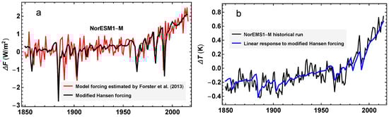
Figure 1.
(a) The red curve is the adjusted forcing for the NorESM1-M model provided by Forster et al. [15]. The black curve is the forcing data of Hansen et al. [16] modified so that its 17-year moving average equals the 17-year moving average of the red curve. (b) The black curve is the global surface temperature in the historical run of the NorESM1-M model, and the blue curve is the response to the modified Hansen forcing (the black curve in (a)) for the model given by Equation (5). Parameters are estimated as and y.
When parameters and are estimated for the historical runs of each ESM, the estimated scale dependent sensitivity can be computed for each model using Equation (6). The factor is taken individually for each model based on the Gregory estimates in [1]. A scalar metric R is obtained by evaluating the functions at the frequency y. The results are presented in Table 1. The choice of frequency is based on how well the corresponding scalar metric correlates with the Gregory estimates of ECS. The scale-dependent sensitivities are computed from Equation (6) under the assumption that the response function is scaling and given by Equation (5). Hence the -curves are power-laws and displayed as the straight, sloping lines in the double-logarithmic plot in Figure 2a. The figure shows that over the model ensemble, typically equals the Gregory estimate of ECS for frequencies y, and Figure 2b shows that the correlation (over the model ensemble) between and the Gregory estimate of ECS has its maximum for y. The falling correlation for lower f suggests that the power-law assumption for fails for time scales much longer than a millennium.

Table 1.
Estimated quantities for the Earth system model (ESM) in the ensemble. The columns for equilibrium climate sensitivity (ECS) and are obtained from Gregory plots for 4 × CO runs and taken from [1]. The columns denoted , and show the estimates of the parameters in the model given by Equation (2) with response function given by Equation (5), obtained from historical runs of the ESMs and the modified Hansen forcing for each model. The last column displays the scale-dependent sensitivity obtained from Equation (6) using the values of , and that are listed in the columns to the left, and evaluated at y.
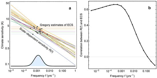
Figure 2.
(a) The sloping lines are double-logarithmic plots of the scale dependent sensitivity for each ESM in the ensemble. The different slopes correspond to different -estimates. The horizontal lines indicate the ECS of the ESMs obtained from the Gregory plots and reported in [1], and the black dots indicate for which frequency f we have for each model. (b) Correlation (over the ensemble of ESMs) between the scale-dependent sensitivity and the Gregory estimate of the ECS. The correlation coefficient is plotted as a function of the frequency f.
Figure 3a shows a plot of the R, i.e., evaluated at y, versus the Gregory estimate of ECS. The points (letters) represent the different ESMs in the model ensemble, and the contour plot shows the conditional probability density function (PDF) estimated from the seventeen data points corresponding to the seventeen ESMs in the ensemble. The method used to estimate is the same as prescribed by Cox et al. (2018) [9], with the obvious weakness that it is based on the assumption that the deviation among the models from an emergent linear relationship between ECS and R has a Gaussian distribution.
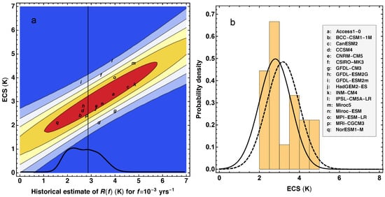
Figure 3.
(a) The letters (see the legend inserted in panel (b)) show the Gregory estimate of ECS versus R(f)m evaluated at y for each model in the ensemble. The contour plot shows the conditional probability density function (PDF) . The vertical black line is K, which is obtained from the parameters and y estimated from the instrumental temperature record using the Hansen forcing. The thick, black curve is the estimated PDF of . (b) The full curve shows the PDF for ECS computed from Equation (14), where is the PDF shown in (a). The histogram is the distribution of ECS in the model ensemble, and the dotted curve is a Gaussian fit to the histogram.
The vertical black line in Figure 3a is K. This value of R is obtained from the parameters and y, which are estimated from the instrumental temperature record using the Hansen-forcing. We have used W/m, which is the value for the GISS-E2-R model given in Table 1. Hence this value for R is the one estimated for the effective forcing used in this particular model and applied to the observed temperature time series. Similar estimates are made for the adjusted forcing in all the other models, using the values of for those models given in Table 1. The black curve in the lower part of Figure 3a is a PDF for the metric R estimated this way. The PDF is obtained by considering two sources of uncertainty in the R-estimates. One is the spread in parameter estimates when we vary the forcing. The forcing is varied over the set of modified Hansen forcing time series, where each modification corresponds to a historical run of an ESM in the ensemble. The parameter estimates for the instrumental temperature record, and the resulting value of R, for varying forcing data is shown in Table 2. Another source of uncertainty is the spread in the parameters and across repeated historical runs of the same model, i.e., runs where the known forcing is the same, but where chaotic dynamics create random components that vary among realizations. Table 3 shows a set of parameter estimates for repeated historical runs of the CSIRO model, which is the model in the CMIP5 ensemble that provides the largest number of runs with identical forcing. The total variability from these two sources is obtained by a simple mixture model, and the plotted PDF is computed by a smooth kernel method. The black, full curve in Figure 3b shows the PDF for ECS computed from the formula
where is the PDF shown in Figure 3a. The histogram in Figure 3b is the distribution of ECS in the model ensemble, and the dotted curve is a Gaussian fit to the distribution of ECS in the model ensemble. The figure demonstrates that when constrained by the scale-dependent sensitivity of the instrumental temperature record, the best estimate of ECS in the model ensemble is reduced by approximately K. The PDF shown in Figure 3a, also shows that, with the uncertainties taken into account, models with ECS larger than 4 K are inconsistent with the instrumental temperature record.
Table 2.
The parameter estimates for the instrumental temperature record, and the resulting values of R, for varying forcing data.
Table 3.
A set of parameter estimates for repeated historical runs of the CSIRO model.
From Figure 3a and Equation (14) we observe that the uncertainty represented by in Figure 3b is formed by a combination of the range of R-values R represented by the black curve for in Figure 3a and the width of the conditional PDF represented by the contour lines in that panel. The latter represents the uncertainty associated with the deviation from the emergent linear relation between ECS and R among the models, which is the main source of uncertainty found by Cox et al. (2018) [9]. In our approach, however, the wide range of the metric R represented by that we have found by using the adjusted forcing of each model to estimate R is a major contribution to the uncertainty in .
One can explore the effect of uncertainty of adjusted forcing among models on the uncertainty of ECS by neglecting the uncertainty associated with deviations from the emergent linear relation. From the scatter plot in Figure 3a we can fit a linear relationship , and in Table 2 we have a set of estimates of R for the instrumental temperature record. The linear fit maps each of the R-estimates to an ECS-value, which can be interpreted as the best estimate of ECS based on the corresponding forcing data. This mapping is shown in Figure 4a. The range of these best estimates of ECS are between 2.3 and 3.4 K. Note that these are the best estimate of R for each model and that the uncertainty of each estimate arising from uncertainty in estimates of and is not taken into account. For this reason, we don’t plot PDFs, but only indicate the range of best estimates of R.
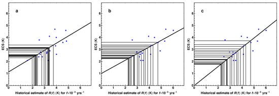
Figure 4.
(a) The points in the scatter plot are the same as (the letters) in Figure 3a. The line is the least-square fit of the model . The vertical lines correspond to the R-values estimated from the instrumental temperature record for the different modified Hansen forcing time series. The horizontal lines show how these R-values are mapped to ECS-values by the linear model. (b) As in (a), but prior to the analysis the volcanic forcing is reduced to half of its original values. (c) As in (b), but using a linear model with zero intercept to map R-values to ECS-values.
The effect of uncertainty in the forcing on the estimated ECS can be explored further by varying the various forcing components within plausible ranges of uncertainty. As an example we consider the forcing from volcanic aerosols, which are subject to considerable controversy. In Figure 4b we have made the same plot as in Figure 4a, but with the volcanic component of the Hansen forcing reduced by 50 percent. The effect on the spread in the estimated ECS is considerable. Another source of uncertainty is the choice of regression model for the emergent relation between ECS and R. From a physical viewpoint, vanishing ECS should correspond to vanishing R, so if one sticks to a linear model it could be reasonable to choose the model rather than . The result for such a model, keeping the low volcanic forcing, is shown in Figure 4c, with a range of best estimates for ECS between 1.8 and 3.7 K.
5. Discussion
The PDF for the ECS shown in Figure 3b is similar to the one presented by Cox et al. [9]. However, there are important differences in methodology that must be pointed out. Cox et al. use a pure dissipation-response relationship to constrain ECS in the model ensemble. They propose a metric , which plays a similar role as the metric R proposed in this work, and claim that estimates of are independent of the forcing. This claim has been demonstrated to be false [10]. In our framework, an approach in the spirit of Cox et al. would be to use Equation (10), and to seek estimates of the correlation function (or equivalently the PSD) of the climate noise that are independent of the forcing. Such an approach would lead to the same problems as those in [9], namely that the estimates would be influenced by the strong anthropogenic forcing in the instrumental period. This is our motivation for developing a method that employs forcing data in the estimation of our metric R, and as a consequence we have to take the uncertainty in the forcing into account. We have done this by using a fixed data set for historical forcing (the Hansen-forcing) and varied its low-frequency variability over the ensemble of adjusted forcing time series provided by Forster et al. [15]. Clearly, this does not represent the full uncertainty in the historical forcing, and hence the spread in the distribution of ECS (the black, full curve in Figure 3b) is narrower than what we expect to find if we were to model the full forcing uncertainty. We conclude that accurate estimates of the uncertainty in historical forcing is a key factor for establishing constraints on ECS in ESM ensembles.
The modeling of the relationship between R and ECS is also a source of uncertainty. It is evident from Figure 4a that the coefficient a in the linear map is less than one. In fact, its estimated value is . As a consequence the mapping from R to ECS is contracting, so that the spread in ECS-values is smaller than the spread in R-values. The same is true for the analysis presented in Figure 3, since the conditional PDF is constructed from the fitted line . We note that for a model without the intercept term b, and lower volcanic forcing, the estimated coefficient is , and the range of the best estimates of ECS becomes 1.8–3.7 K. Other assumptions about the functional relationship between R and ECS will lead to yet different ranges of best estimates.
Apart from the constraints on ECS, an important result presented in this paper is that scale-dependent climate sensitivity provides a good proxy for ECS. Moreover, despite having infinite ECS, scale-invariant linear response models are useful for estimating ECS from observational data. The advantage over multi-layer energy balance models is that the scale-invariant models have few free parameters and are less prone to statistical overfitting. The accuracy of the models is associated with the scaling nature of climate variability, an emergent property of the complex climate system.
Author Contributions
All authors conceived and designed the study; H.-B.F. collected data and constructed the modified forcing data. E.M.-N. and S.H.S. performed the parameter estimates; M.R. and H.-B.F. analyzed the results; M.R. and K.R. wrote the paper with input from all authors.
Funding
This research received no external funding.
Conflicts of Interest
The authors declare no conflict of interest.
Abbreviations
The following abbreviations are used in this manuscript:
| ECS | Equilibrium climate sensitivity |
| ESM | Earth system model |
| IPCC | Intergovernmental Panel on Climate Change |
| GMST | Global mean surface temperature |
| CERES | Clouds and Earth’s Radiant Energy System |
| CMIP5 | Coupled Model Intercomparison Project Phase 5 |
| ENSO | El Niño Southern Oscillation |
| PSD | Power Spectral Density |
| LRD | Long-range dependence |
| fGn | fractional Gaussian noise |
| Probability density function | |
| INLA | Integrated nested Laplace approximation |
References
- IPCC. Climate Change 2013: The Physical Science Basis. Contribution of Working Group I to the Fifth Assessment Report of the Intergovernmental Panel on Climate Change; Cambridge University Press: Cambridge, UK, 2013. [Google Scholar]
- Gregory, J.M.; Ingram, W.J.; Palmer, M.A.; Jones, G.S.; Stott, P.A.; Thorpe, R.B.; Lowe, J.A.; Johns, T.C.; Williams, K.D. A new method for diagnosing radiative forcing and climate sensitivity. Geophys. Res. Lett. 2004, 31, L03205. [Google Scholar] [CrossRef]
- Knutti, R.; Rugenstein, M.A.; Hegerl, G.C. Beyond equilibrium climate sensitivity. Nat. Geosci. 2017, 10, 727–736. [Google Scholar] [CrossRef]
- Von der Heydt, A.S.; Köhler, P.; van de Wal, P.R.S.W.; Dijkstra, H.A. On the state dependency of fast feedback processes in (paleo) climate sensitivity. Geophys. Res. Lett. 2014, 41, 6484–6492. [Google Scholar] [CrossRef]
- Von der Heydt, A.S.; Dijkstra, H.A.; van de Wal, R.S.W.; Caballero, R.; Crucifix, M.; Foster, G.L.; Huber, M.; Köhler, P.; Rohling, E.; Valdes, P.J.; et al. Lessons on Climate Sensitivity From Past Climate Changes. Curr. Clim. Chang. Rep. 2016, 2, 148–158. [Google Scholar] [CrossRef]
- Von der Heydt, A.S.; Ashwin, P. State dependence of climate sensitivity: Attractor constraints and palaeoclimate regimes. Dyn. Stat. Clim. Syst. 2017, 1, 1–21. [Google Scholar] [CrossRef]
- Köhler, P.; Stap, L.B.; von der Heydt, A.S.; de Boer, B.; van de Wal, R.S.W.; Bloch-Johnson, J. A State-Dependent Quantification of Climate Sensitivity Based on Paleodata of the Last 2.1 Million Years. Paleoceanography 2017, 32, 1102–1114. [Google Scholar] [CrossRef]
- Dessler, A.E.; Forster, O.M. An estimate of equilibrium climate sensitivity from interannual variability. J. Geophys. Res. Atmos. 2018. [Google Scholar] [CrossRef]
- Cox, P.M.; Huntingford, C.; Williamson, M. Emergent constraint on equilibrium climate sensitivity from global temperature variabilit. Nature 2018, 553, 319–322. [Google Scholar] [CrossRef] [PubMed]
- Rypdal, M.; Fredriksen, H.B.; Rypdal, K.; Steene, R.J. Emergent constraints on climate sensitivity. Nature 2018. [Google Scholar] [CrossRef] [PubMed]
- Fredriksen, H.B.; Rypdal, M. Long-range persistence in global surface temperatures explained by linear multibox energy balance models. J. Clim. 2017, 30, 7157–7168. [Google Scholar] [CrossRef]
- Rypdal, M.; Rypdal, K. Long-memory effects in linear response models of Earth’s temperature and implications for future global warming. J. Clim. 2014, 27, 5240–5258. [Google Scholar] [CrossRef]
- Myhre, G.; Myhre, C.L.; Forster, P.M.; Shine, K.P. Halfway to doubling of CO2 radiative forcing. Nat. Geosci. 2017, 10, 710–711. [Google Scholar] [CrossRef]
- Andrews, T.; Gregory, J.M.; Webb, M.J.; Taylor, K.E. Forcing, feedbacks and climate sensitivity in CMIP5 coupled atmosphere-ocean climate models. Geophys. Res. Lett. 2017, 39, L09712. [Google Scholar] [CrossRef]
- Forster, P.M.; Andrews, T.; Good, P.; Gregory, J.M.; Jackson, L.S.; Zelinka, M. Evaluating adjusted forcing and model spread for historical and future scenarios in the CMIP5 generation of climate models. J. Geophys. Res. Atmos. 2013, 118, 1139–1150. [Google Scholar] [CrossRef]
- Hansen, J.; Sato, M.; Kharecha, P.; von Schuckmann, K.; Beerling, D.J.; Cao, J.; Marcott, S.; Masson-Delmotte, V.; Prather, M.J.; Rohling, E.J.; et al. Young people’s burden: Requirement of negative CO2 emissions. Earth Syst. Dyn. 2017, 8, 577–616. [Google Scholar] [CrossRef]
- Rypdal, M.; Rypdal, K. Late Quaternary temperature variability described as abrupt transitions on a 1/f noise background. Earth Syst. Dyn. 2016, 7, 281–293. [Google Scholar] [CrossRef]
- Rybski, D.; Bunde, A.; Havlin, S.; von Storch, H. Long-term persistence in climate and the detection problem. Geophys. Res. Lett. 2006, 33, L06718. [Google Scholar] [CrossRef]
- Lovejoy, S.; Schertzer, D. The Weather and Climate: Emergent Laws and Multifractal Cascades; Cambridge University Press: Cambridge, UK, 2013. [Google Scholar]
- Huybers, P.; Curry, W. Links between annual, Milankovitch and continuum temperature variability. Nature 2005, 441, 329–332. [Google Scholar] [CrossRef] [PubMed]
- Franzke, C. Long-Range Dependence and Climate Noise Characteristics of Antarctic Temperature Data. J. Clim. 2010, 23, 6074–6081. [Google Scholar] [CrossRef]
- Fredriksen, H.B.; Rypdal, K. Spectral characteristics of instrumental and climate model surface temperatures. J. Clim. 2016, 29, 1253–1268. [Google Scholar] [CrossRef]
- Rypdal, K.; Rypdal, M.; Fredriksen, H.B. Spatiotemporal long-range persistence in earth’s temperature field: Analysis of stochastic-diffusive energy balance models. J. Clim. 2015, 28, 8379–8395. [Google Scholar] [CrossRef]
- Rypdal, K. Global temperature response to radiative forcing: Solar cycle versus volcanic eruptions. J. Geophys. Res. Atmos. 2012, 117, D06115. [Google Scholar] [CrossRef]
- Mandelbrot, B.; Ness, J. Fractional Brownian motions, fractional noises and applications. SIAM Rev. 1968, 18, 1088–1107. [Google Scholar] [CrossRef]
- Rue, H.; Martino, S.; Chopin, N. Approximate Bayesian inference for latent Gaussian models using integrated nested Laplace approximations (with discussion). J. R. Stat. Soc. Ser. B 2009, 71, 319–392. [Google Scholar] [CrossRef]
- Sørbye, S.H.; Myrvoll-Nilsen, E.; Rue, H. An approximate fractional Gaussian noise model with (n) computational cost. Stat. Comput. 2017. [Google Scholar] [CrossRef]
- Myrvoll-Nilsen, E.; Sørbye, S.H.; Rypdal, M.; Fredriksen, H.B.; Rue, H. Method for estimating climate response under scaling assumption. 2018. preprint. [Google Scholar]
© 2018 by the authors. Licensee MDPI, Basel, Switzerland. This article is an open access article distributed under the terms and conditions of the Creative Commons Attribution (CC BY) license (http://creativecommons.org/licenses/by/4.0/).