Article

Aero-Engine Preliminary Design Optimization and Operability Studies Supported by a Compressor Mean-Line Design Module

by
Alexios Alexiou
*,
Ioannis Kolias
,
Nikolaos Aretakis
and
Konstantinos Mathioudakis
Laboratory of Thermal Turbomachines, School of Mechanical Engineering, National Technical University of Athens, 15780 Athens, Greece
*
Author to whom correspondence should be addressed.
Aerospace 2023, 10(8), 726; https://doi.org/10.3390/aerospace10080726
Submission received: 28 June 2023 / Revised: 10 August 2023 / Accepted: 18 August 2023 / Published: 20 August 2023
(This article belongs to the Special Issue Aerodynamic and Multidisciplinary Design Optimization)

Abstract

:
An approach for preliminary aero-engine design, incorporating a mean-line code for the design of axial-flow, multi-stage compressors, is presented. The compressor mean-line code is developed and integrated within a framework for the preliminary design and assessment of aero-engine concepts. It is then combined with modules for compressor map generation, multi-point engine design, steady-state and transient engine off-design performance and aircraft mission analysis. Implementation examples are presented, demonstrating the determination of the optimal combination of compressor and engine design parameters for achieving minimum fuel burn over a specific aircraft mission, while obeying constraints that guarantee operability over the entire flight envelope. Constraints related to compressor stability during transient maneuvers between idle and static take-off conditions and engine temperature limits at maximum take-off are respected by the final design. The results demonstrate the potential for design trade-offs between engine performance at the aircraft mission level and compressor aerodynamic stability.

1. Introduction

One of the near-term technologies pursued by the aviation industry, for reducing its environmental footprint, is through transitioning to ultra-high bypass ratio (UHBR) geared turbofan concepts [1,2,3]. Combined with increases in overall pressure ratio (OPR), improvements in both propulsive and thermal efficiencies can be achieved, thus leading to a reduction in fuel consumption and, hence, CO2 emissions. Upper limits on bypass ratio (BPR) and OPR values are dictated by, among others, the ability to reach acceptable levels of idle thrust during descent, approach and on the ground, as well as meeting performance requirements set by certification authorities and aircraft operational constraints, regarding maneuvers between low- and high-power conditions. Idle thrust levels and response times are related to engine operability and especially compressor stability at low power. UHBR layouts are designed with large low-pressure systems and small cores, giving rise to mismatch between low- and high-pressure spool inertias, which are prime factors in determining transient compressor response, thus making the fulfilment of aircraft descent and go-around requirements more challenging. UHBR engine preliminary design must, thus, consider idle thrust and transient performance, to ensure that its fuel-burn potential benefits can actually be achieved. Indeed, this type of analysis is relevant to all future engine concepts currently being considered, such as hybrid-electric, open rotor, etc.
Dynamic analysis of an advanced geared turbofan UHBR engine was performed in [4] and revealed that the HPC transient stack needed to meet the FAA 5s certification requirement [5] allows for a lower steady-state surge margin constraint, compared to that used for the engine design. It was concluded that this would potentially have resulted in significant efficiency improvements, if the engine design process was performed again.
A methodology for aero-engine preliminary design that integrates transient performance is presented in [6]. Its applicability is demonstrated for the case of a generic turbofan configuration through a parametric analysis in order to show the effects of selected HP compressor design parameters on transient performance.
The group of authors highlighted the need to integrate transient analysis in the overall engine design optimization process, in order to avoid a redesign in case of non-compliance. This was demonstrated via a transient performance assessment against the FAA 5s certification maneuver of a UHBR engine optimized for minimum fuel burn [7].
The present paper extends the multi-disciplinary preliminary design optimization framework of [7], with the inclusion of compressor mean-line design and analysis modules and closes the loop with transient performance, by integrating it in the overall aircraft-level optimization scheme.
A key enabler for compressor stability studies at the engine and aircraft level is the ability to conduct compressor design via a mean-line (1D) module, at the preliminary design stage. In the context of engine design and optimization, it accounts for changes in cycle parameters (e.g., pressure ratio) and allows compressor flow and geometrical parameters that affect performance and operability, to be considered as design choices. It derives the compressor geometry, which is then used to generate consistent performance maps to be used by the engine module that evaluates steady-state and transient performance.
Before presenting the overall design framework, the formulation, implementation and validation of an axial-flow, multi-stage compressor module, called MLDC (Mean-Line Design Code) is described. Its integration into a UHBR engine design optimization test case is then exemplified. The objective of the study is to establish the combination of selected compressor and engine cycle design parameters for minimum aircraft mission fuel burn, while meeting engine response requirements, without violating compressor stability limits and engine aero-thermodynamic and structural constraints.

2. MLDC Formulation, Validation, and Integration

Compressors are probably the most critical components for the overall operation of an engine. Understanding the flow aerodynamics through compressors continues to trouble numerous teams of researchers and engineers, throughout industry and academia. The difficulty in fully understanding the physics of the flow across compressors has made their design and off-design performance modelling and prediction, as well as their structural design, challenging tasks [8]. Teams from both industry and academia have put significant effort in developing tools for the accurate modelling and prediction of compressor performance. Such tools need to be fast, reliable, and sufficiently accurate already from the preliminary design phase. During this phase, tools should also require the minimum number of inputs and the minimum effort to set up a calculation case. Their integration in frameworks for the overall design and assessment of new engines should also be easy. For these reasons, mean-line models (1D) are of great use and continue to be preferred over lower- (0D) and higher-fidelity (2D/3D) tools for the preliminary design and analysis of compressors [9,10,11,12,13,14,15,16,17,18,19,20,21,22,23,24,25,26,27,28,29,30,31,32].
A 1D design code should produce the compressor flowpath for the specified mass flow and design pressure ratio, with the maximum efficiency and the minimum number of stages. This should be performed while producing consistent blade dimensions to be subsequently used as inputs to the detailed design, thus minimizing the iterations between preliminary and detail design phases. However, due to the high complexity of the flow physics involved, these objectives can only be met if a code is sufficiently versatile by including the possibility for different design options and calculation inputs, blade models, loss sources and/or models, etc. An analysis mode is also a desirable feature for the consistent prediction of the compressor off-design performance over a range of working conditions, once the design has been concluded.
In the past, many design methodologies and tools for both teaching [18,19,20,21,22,23,24,25] and research [26,27,28,29,30,31,32] have been proposed. However, all codes present limitations which, in turn, reduce their automation, versatility, and design capability. Limitations encountered at various publications are
  • The design inputs may be pre-fixed (e.g., in [18,19,25]) and, if the user wishes to modify them, then the entire code has to be re-compiled.
  • The compressor efficiency may be an input (e.g., in [24,27]), that is, it is not estimated based on the flow losses across the compressor.
  • In all the above codes, the compressor design is conducted in a stage-by-stage manner where the number of stages is an input. In other words, the number of stages is not obtained on the basis of physical principles, such as the stage-wise loading and loss distributions for achieving the desired design pressure ratio.
  • The compressor design relies on simplifying assumptions, e.g., repeating stages in [18,19,25] or constant enthalpy change per stage in [27].
  • Commonly, the compressor design is limited to three flowpath shapes (constant hub, mean, and tip). In some codes, the user may also need to specify the value of certain flowpath diameters (e.g., in [26]), that is, the flowpath geometry is not obtained entirely from the aerodynamic design.
  • The blade row losses may be an input (e.g., in [18,19,20,21,22,23,26,32]) while, in most codes, losses from only two sources (profile and shock) are accounted for (e.g., in [24,29,30,31]). In all cases, losses are estimated from pre-defined models, that is, the user cannot select from different loss models.
  • Blade geometry and performance are commonly defined considering only two blade models, the NACA-65 for subsonic flows and DCA for transonic flows (e.g., in [29,30,31]).
  • The work distribution may be an input (as, e.g., in [30,32]). That is, it is not obtained from aerodynamic criteria regarding the loading of the blades (e.g., loading coefficient, minimum De Haller number, maximum diffusion factor, maximum flow turning, etc.).
  • Finally, hardly any code combines an analysis mode for producing consistent performance maps after the compressor design has been completed. The only exception are the codes presented in [26,28], but even for these there is no indication by their authors that the design and analysis modes cooperate or that they use consistent physical assumptions, fluid models, thermodynamic functions, and numerical solvers.
MLDC overcomes the abovementioned limitations by offering to the user a variety of input and calculations options, as described in the following paragraphs.
MLDC is developed in the same modelling environment as conventional 0D engine components, thus using the same interface, fluid and thermodynamic functions and numerical routines while inheriting directly the basic modelling equations of 0D general purpose turbomachinery components. It uses the same fluid models, thermodynamic functions, blade models, loss models, and numerical schemes as those employed in the Mean-Line Analysis Code (MLAC) for compressor off-design performance predictions described previously by the authors [9]. Thus, MLDC produces compressor geometries, which can then be used by MLAC to generate consistent performance maps. Modelling and numerical homogeneity are thus ensured, allowing the transparent and consistent integration of mixed-fidelity components either directly at the engine level or as part of a simulation flow process.
An example of the latter is presented in this paper for demonstrating the use of MLDC in a design optimization test case that combines modules for 1D compressor design (MLDC) and analysis (MLAC), aero-thermodynamic, multi-point engine design, steady-state and transient off-design engine performance and aircraft mission analysis.

2.1. MLDC Formulation and Design Options

MLDC establishes the compressor geometry and performance by conducting a row-by-row calculation, where the flowpath and blade dimensions are derived simultaneously. The flowpath radii are obtained by the aero-thermodynamic design of the blade rows, and then they are used to obtain basic blade dimensions such as blade heights and chord lengths. The latter are then used to axially size the compressor flowpath, thus moving the design sequence to the next row. For this calculation, the user must specify the compressor inlet conditions ( m ˙ , T 0 , p 0 ), the compressor speed in the form of N m e c h or U 1 , t or both (in the latter case the compressor inlet hub-to-tip ratio is obtained), and the compressor design pressure ratio.
Calculation approaches, design assumptions and user options for establishing the compressor geometry at component and at blade row level are described in the following.

2.1.1. Meridional Compressor Design

For a given pressure ratio ( Π C ), the compressor design is conducted following one of two possible approaches. In the first one, the number of stages is specified by the user. In the second, the number of stages is an output of the aero-thermodynamic design, as MLDC accumulates stages until the required Π C is achieved. In either case, if for the current work distribution Π C is exceeded, then a follow-on calculation adjusts the overall compressor enthalpy change (for the same work distribution) in order to match the required Π C .
The work distribution, expressed as percentage of stage enthalpy rise to compressor overall enthalpy rise, can either be an input or can be established according to all or any of the following four aerodynamic criteria [33]:
  • Maximum diffusion factor at rotor tip (default value = 0.50);
  • Maximum diffusion factor at stator hub (default value = 0.60);
  • Maximum turning flow angle at rotor hub (default value = 40°);
  • Maximum Mach number at stator hub (default value = 0.85).
In order to establish the compressor work distribution and the corresponding operating conditions of the blade rows, the axial velocity distribution and the rotor inlet absolute flow angle are also needed. Appendix A describes the calculation options available in MLDC, for these parameters.
In MLDC, the compressor flowpath shape can be described by choosing one among the following eight ways:
  • Constant hub radius;
  • Constant mean radius;
  • Constant tip radius;
  • Mean radius distribution as a ratio from the average value;
  • Constant radius from compressor’s inlet up to a stage and then linear up to exit;
  • Linear from compressor’s inlet up to a stage and then constant up to exit;
  • Mean radius distribution between the inlet and exit using a single user-defined parameter that, similarly to option 1 in Appendix A, for the definition of the axial velocity distribution, describes the shape of a parabola in relation to a straight line;
  • User-specified mean radius distribution.
Additionally, the user must specify the compressor inlet hub-to-tip ratio, except when both N m e c h and U 1 , t are specified. The exit hub-to-tip ratio is only required when the flowpath shape is defined according to choices 5–7.
Having determined the compressor flowpath radii, axial sizing is conducted employing an adapted version of the methodology presented in [19]. The axial gap percentage between two consecutive blade rows is either an input or obtained considering linear interpolation between a first and last row input value. This is defined as the axial gap length divided by the average value of the hub and tip axial chord lengths of the upstream row. For rows where bleeds occur, the axial gap is set explicitly to facilitate the necessary mass extraction. Typical values for axial gap percentages can be found in [34].

2.1.2. Blade Row Design

For predicting the flow ( m ˙ , T 0 , p 0 ) across any blade row and for estimating the required geometry, MLDC employs the same computational building blocks as those used in MLAC [9], i.e., the Blade Row Module (BRM) and the Inter-Volume Module (IVM). Figure 1 illustrates the blade row modelling concept through BRMs and IVMs.
IVM models the flow in the duct after a blade row. In IVM, gas bleeds are taken into account through mass and gas composition continuity, while flowpath radius changes are accounted for through a moment of momentum balance:
( m ˙ R m V θ ) 3 = ( m ˙ R m V θ ) 2
In IVM, pressure losses, heat transfer effects, and gas mixing through water-vapor injection have also been foreseen.
BRM establishes the performance (flow losses and deviation) and geometry (metal angles, chord lengths, blade count) of individual blade rows. BRM can model any type of rotating or stationary blade row, of fixed or variable geometry. In MLDC, four profile shapes are available for describing the geometry and performance of a blade section:
  • NACA-65;
  • NACA-63 A4K6 (for IGVs);
  • DCA;
  • BC4.
In BRM, the flow across a blade row is described by a set of equations including the mass and gas composition continuity, the conservation of energy, and loss ( ω ) and deviation ( δ ) correlations for obtaining the flow conditions at the outlet of the blade row knowing the ones at the inlet:
{ p r , 2 0 = ( p r , 2 0 ) i s ω ( p r , 1 0 p 1 s ) , for   rotating   blade   rows p 2 0 = p 1 0 ω ( p 1 0 p 1 s ) , for   stationary   blade   rows
β 2 = κ T E + δ
In Equation (2) profile, shock, secondary, endwall, and clearance losses can be accounted for, while profile losses can also be corrected for Mach number and Reynolds number effects. The user can switch on or off any of these loss sources, can use input values for any individual loss contribution or for the overall loss, or can insert custom loss correlations (e.g., obtained by CFD simulations or experimental measurements). Appendix B summarizes the loss and deviation models available in MLDC.
For establishing the blade metal angles ( κ L E and κ T E ), an iteration scheme on the flow angles at the blade row inlet ( β 1 ) and outlet ( β 2 ) is employed. The residual equations required are given by Equation (3) for the estimated deviation angle ( δ ), while an additional equation requires that the actual incidence is equal to that for which the flow losses across the row are minimum (see Appendix B):
i = i m i n
The methodology to estimate the blade chord at the mean-line from aspect ratio and blade count from blade row solidity is described in Appendix A.
Finally, for obtaining the blade metal angles and chord lengths along the blade span, it is assumed that the flow is approximated by a free-vortex [35]. This condition is described by
d V x d r = 0 , d d r ( r V θ ) = 0

2.2. Compressor Overall Performance

Once aerodynamic design has been completed, a number of overall performance quantities are also established. Among these are the compressor isentropic and polytropic efficiencies, as well as indices describing how far the design operating point is from choke and stall.
For choke, the methodology presented by the authors in [9] for MLAC is also applied in MLDC. For stall, an approach similar to the one presented in [9] for choke was formulated, where appropriate indices ( I ) quantifying how far the operation of any individual blade row is from stall were defined. For the definition of these indices, the user has a number of different possibilities:
  • The actual incidence angle is compared to the incidence angle corresponding to stall, where istall is estimated according to [36] or [37]: I = istalli;
  • The actual diffusion factor is compared to a user-defined maximum diffusion factor corresponding to stall: I = DFmaxDF;
  • The actual velocity ratio is compared to the minimum velocity ratio that the row can handle without stalling, where (W2/W1)min is estimated according to [36,38]: I = W2/W1 – (W2/W1)min.
  • The actual static pressure rise coefficient is compared to the maximum static pressure rise coefficient that the row can attain without stalling, where cp,max is estimated according to [33,39]: I = cp,maxcp.
For the compressor to operate stably, stall indices must be positive ( Ι 0 ). As is the case with choke modelling [9], an overall stall index is defined, which is the minimum value between the stall indices of all blade rows. The minimum stall index is used as an indication of the row which is more likely to stall first. In addition to this approach, an overall stall-margin calculation option is also available to the user, as described in [39].

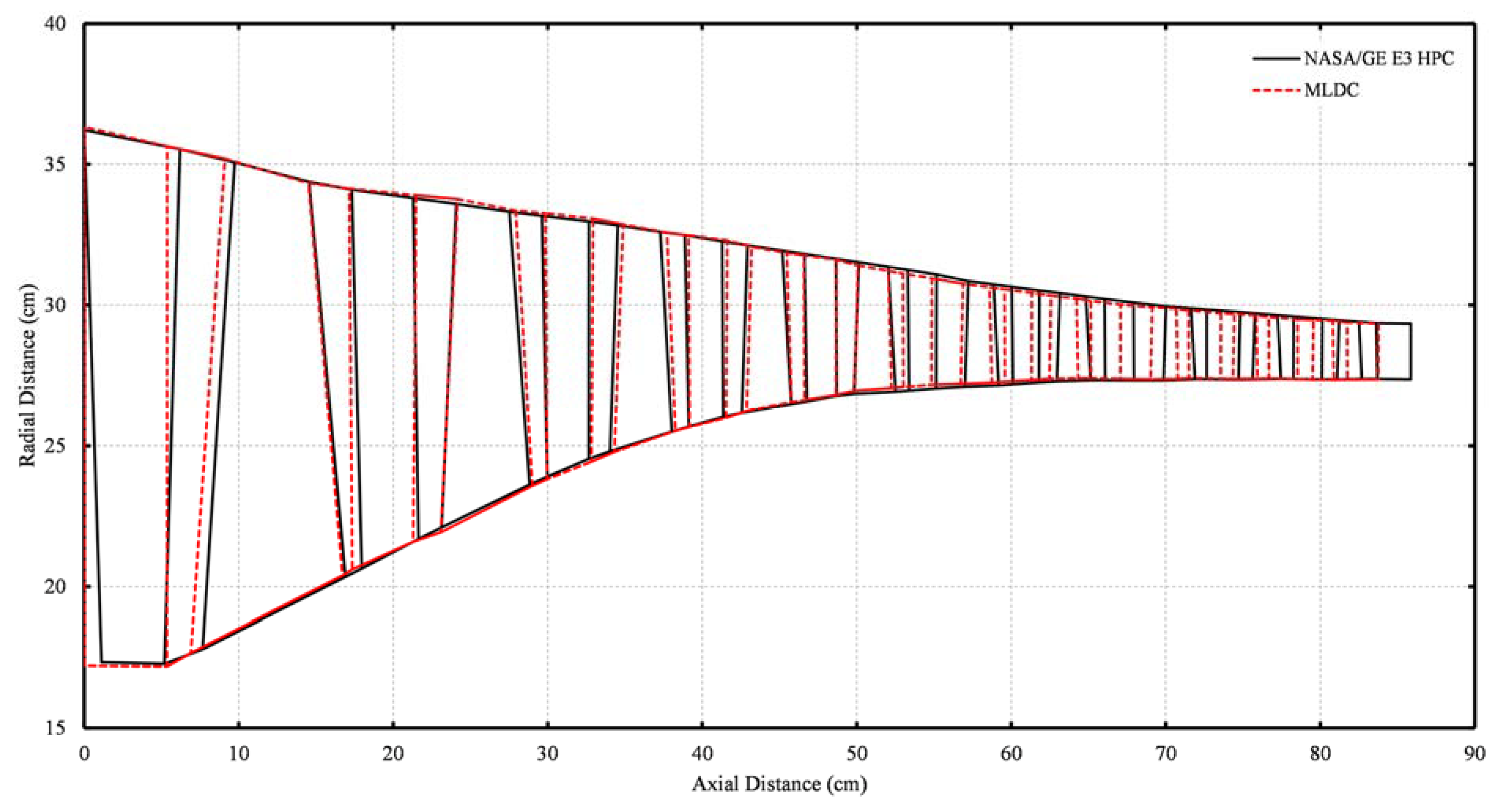
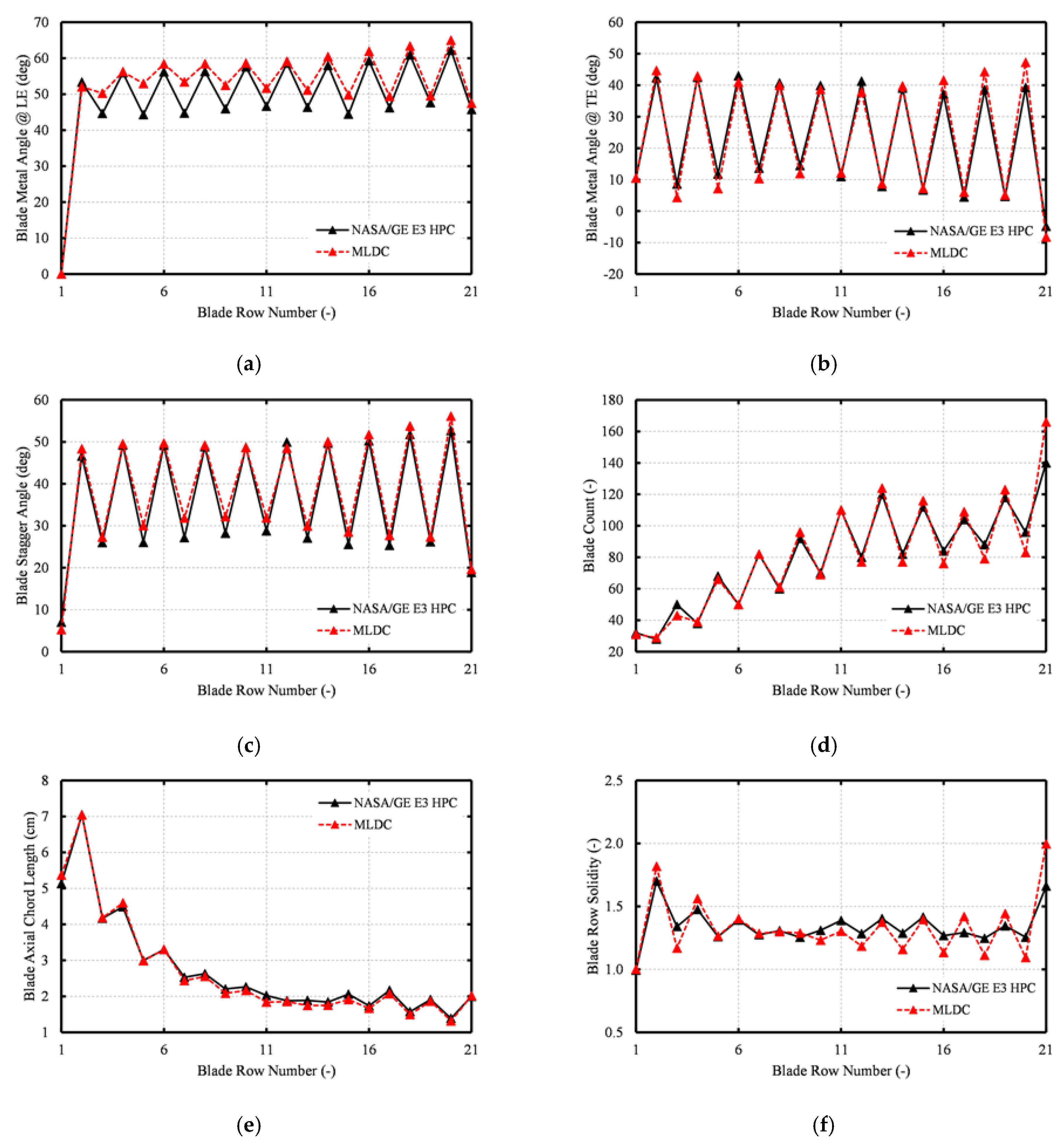
2.3. MLDC Validation

MLDC is validated by comparing its geometry outcome for specific target performance, to the actual geometry of an existing compressor. The well-known NASA/GE E3 HPC is used for this purpose. This is a high-speed and high-aerodynamic loading ten-stage compressor designed and tested during the late 1970s–early 1980s. The aerodynamic design point data for the compressor are summarized in Table 1 [40].
For the validation, the work distribution is determined from the aerodynamic criteria with their default values. The solidity is calculated and the axial velocity distribution at the inlet of the rotors is specified with V ¯ x = 180 m/s (option 2 in Appendix A). The default loss and deviation models seen in Appendix B are used. All other required input parameters (e.g., mean radius distribution, inlet flow angle) are obtained from the relevant public-domain literature [40,41].
The flowpath derived is compared to the actual one in Figure 2 and shows only minor differences along the axial direction due to small differences in the calculation of the chord lengths (Figure 3e) and the way the gap ratio is defined at mean radius in MLDC.
The comparison of other blade row parameters in Figure 3 shows that the blading geometry produced is very close to the actual one, exhibiting an overall axial evolution almost identical to the actual one. Some discrepancies in the geometry produced by a 1D code and the geometry of an actual machine are anticipated, and are related to the simplified flow and geometry modelling used in a 1D code. More specifically, in MLDC the blade metal angle at the leading-edge (Figure 3a) is established numerically and is assumed to be that for which the flow losses across the row are minimum. In an actual machine, the final blade geometry is established based not only on flow considerations, but on manufacturing, maintenance, cost considerations, etc. Another reason for the observed discrepancy could be that in NASA/GE’s E3 HPC, the six (6) first rotor rows are made-up by “special” and “bi-convex” airfoils [40], which are not currently modelled in MLDC. Similarly, discrepancies in solidity (Figure 3f) can be explained by the fact that a simplified semi-empirical correlation is used to establish it.
In the context of preliminary engine design where identifying physical trends is the priority, the level of geometry reconstitution achieved by MLDC demonstrates the validity of its approach for establishing the work distribution and the accuracy of the code as a design tool for axial-flow, multi-stage compressors.

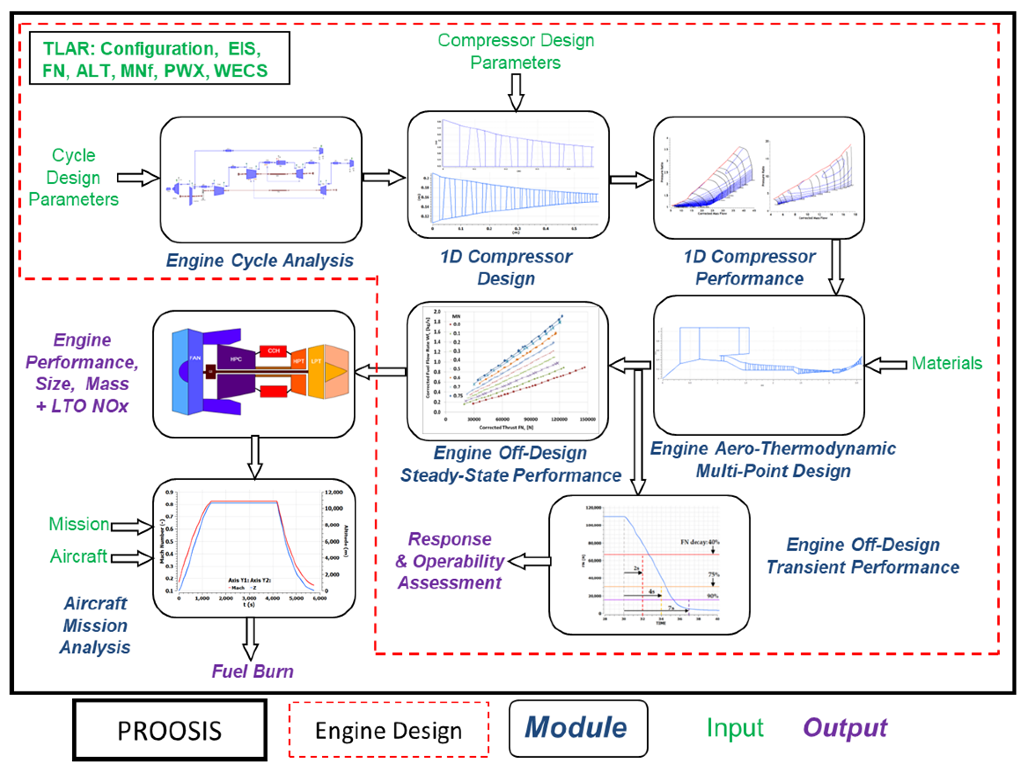
2.4. MLDC Integration into the Framework for the Preliminary Design of Aero-Engines

MLDC was developed and integrated into the framework for the preliminary design and assessment of novel aero-engines that the team of authors has been building in the recent years [7,9,42,43,44], thus enhancing its predictive capabilities. In contrast to other platforms for the preliminary design of gas turbine engines that, commonly, include modules from disparate sources and of proprietary nature (e.g., [27,45,46,47,48,49,50,51,52,53,54,55,56]), it is built under the same coding, modelling, and simulation environment, namely PROOSIS [57]. Therefore, a number of advantages are achieved:
  • The calculation sequence and the data interchange between the different design and analysis modules are transparent, since there is no need for a central data and calculation management system as, e.g., in [52];
  • The physical and mathematical modelling is consistent, since the same fluid properties, thermodynamic functions, numerical schemes, and numerical solvers are implemented in all modules of the framework;
  • The code can be easily maintained and extended, since all modules are developed using the same programming language (PROOSIS’ EL).
Figure 4 depicts the framework and the modules employed in the current application example. The compressor design conditions ( m ˙ , N m e c h , Π C ) are obtained from the engine cycle analysis and are then fed into MLDC for conducting the compressor design. The produced flowpath and blade dimensions are fed into MLAC [9], which uses them to produce consistent performance maps. The maps, in turn, are used by the engine model which conducts the design and off-design steady-state and transient analyses for assessing the overall engine design, stability, and flight performance.

3. Application Example

The framework depicted in Figure 4 was employed for the design optimization of an EIS-2030 geared turbofan configuration with separate, fixed-area bypass and core exhaust nozzles (Figure 5) and for which A320-class aircraft, top-level engine requirements apply in terms of FN, ALT, MNf, ΔT ISA, WECS and PWX. The scope of each module and the flow of information between them can be summarized as follows:
  • Cycle analysis module: this derives the low- and high-pressure compressor design performance ( m ˙ , N m e c h , Π C ) at top-of-climb conditions for a specific set of engine design parameters (BPR, FPR, OPR, nPR and sFN), which are allowed to vary in the context of the fuel-burn optimization calculation.
  • Compressor aerodynamic design module (MLDC): for a set of design choices (e.g., flowpath shape, velocity distribution, inlet/outlet Mach numbers, aspect ratio), it performs the design of the low- and high-pressure compressors. The first rotor tip speed value U1,t and the number of stages Nstg are included in the global optimization variables set. The aerodynamic criteria with their default values are included as constraints.
  • Compressor aerodynamic analysis module (MLAC): this generates the performance maps of the low- and high-pressure compressors for the calculated flowpath geometry and blade rows dimensions established by MLDC. The surge line is established using any of the methods described in the previous section. A variable geometry schedule can be either directly specified or calculated.
  • Aero-thermodynamic multi-point design calculation module: simultaneously solves the three main operating points (top-of-climb, mid-cruise and rolling take-off), produces the engine gas path geometry and estimates values for engine weight, spool inertia and nacelle profile drag coefficient. It also simulates the performance at the ground, descent and approach idle conditions. Constraints in the overall analysis scheme include upper limits on fan diameter (DF), compressor discharge (CDT) and turbine entry temperatures (TET) at the RTO conditions, and lower limits on the HPC ground idle surge margin and HPC last-stage blade height (LSBH). It uses the compressor maps generated by MLAC and feeds the design data to the off-design engine models.
  • Off-design steady-state engine performance module: this runs a series of steady state points for a range of flight conditions and thrust levels to cover the entire operating envelope of the engine. This generates a surrogate engine performance model in the form of a performance table expressing corrected fuel-flow rate for different values of corrected thrust and Mach number values. During this analysis, the Landing and Take-Off (LTO) NOx emissions are also estimated.
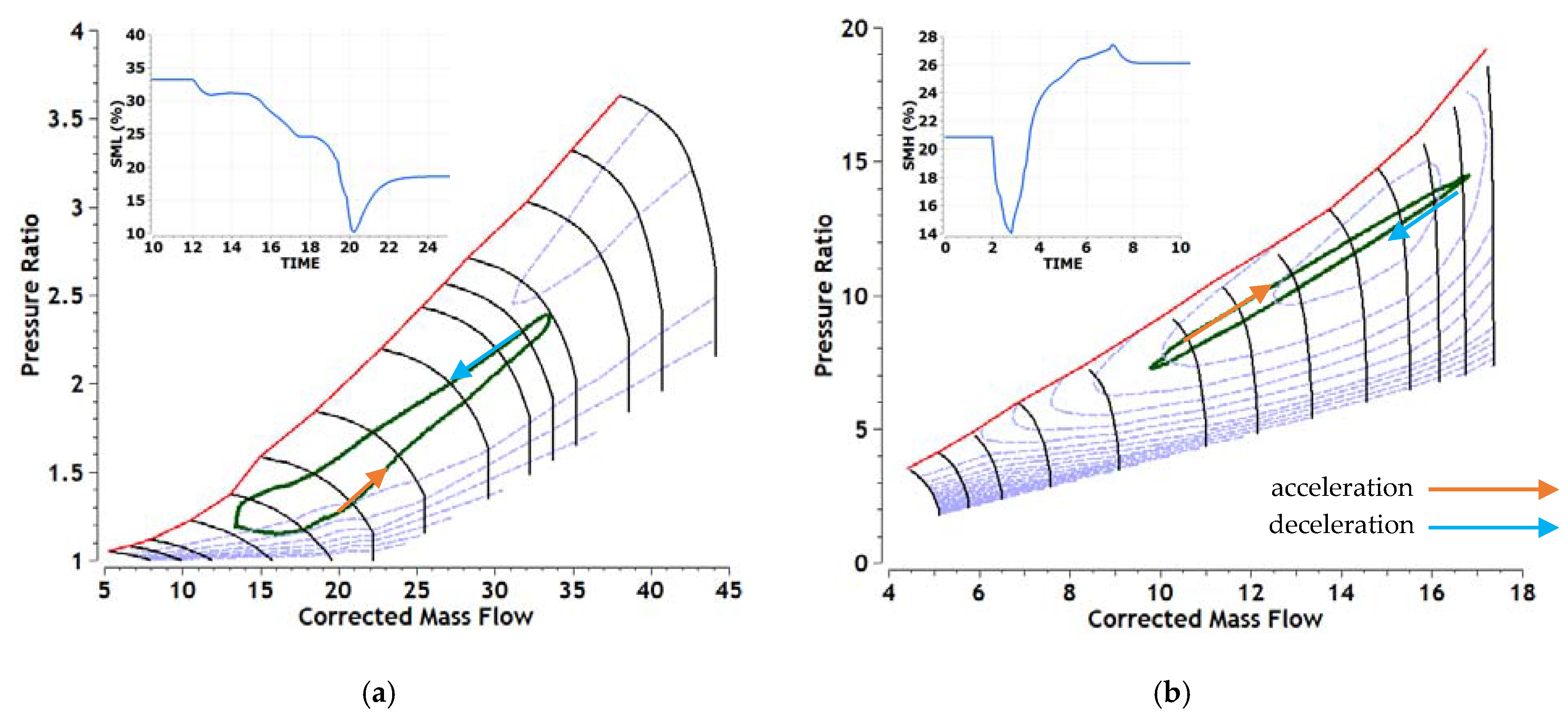
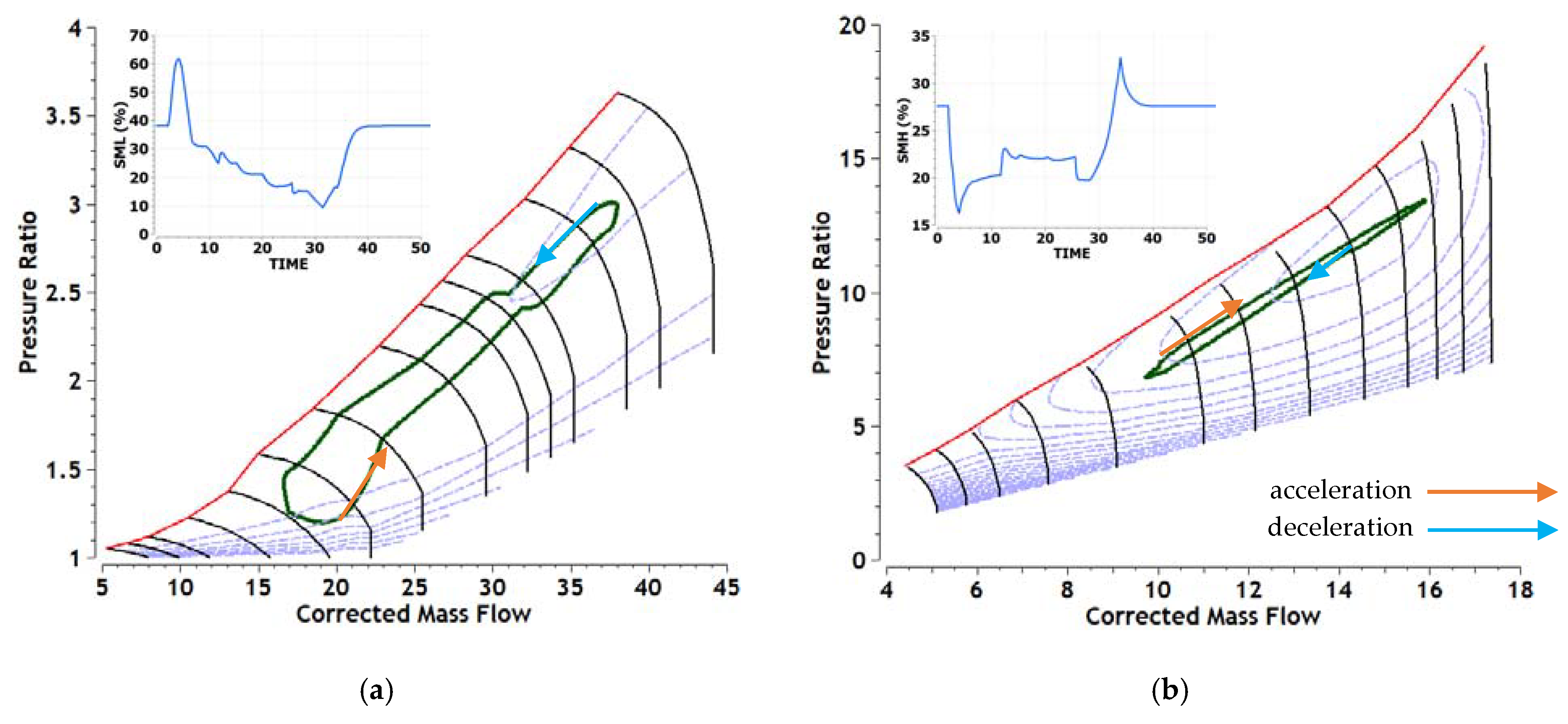
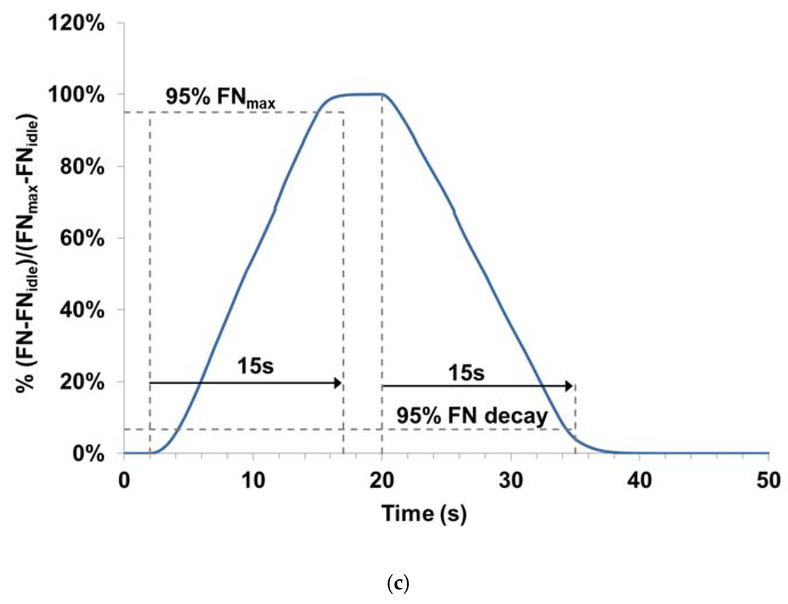
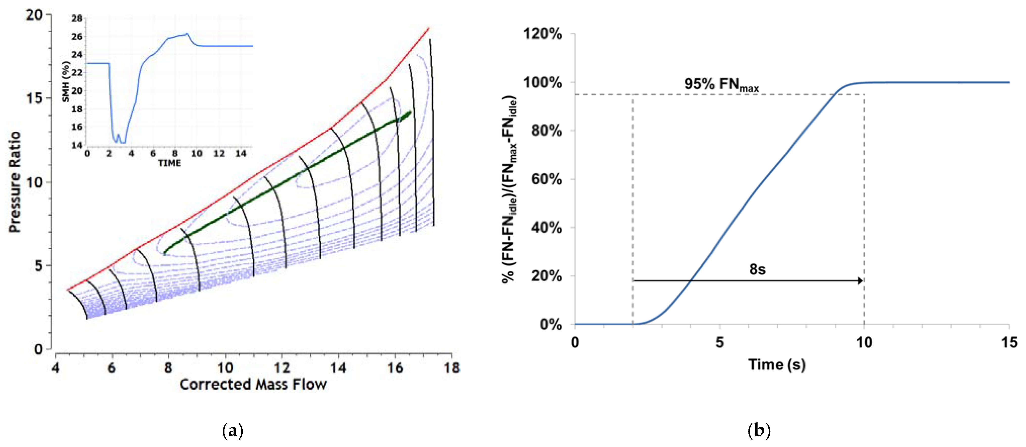
  • Off-design transient engine performance module: this performs a square cycle simulation between 15% and 100% of the rated take-off thrust at sea-level static (SLS) conditions considering spool inertias in order to assess engine response and operability in terms of compressor stability. Minimum acceleration/deceleration thrust margins and LP/HP compressor surge margin limits are included as optimization constraints.
  • Aircraft mission analysis module: using the surrogate engine model, this calculates mission fuel burn for a specific aircraft type and mission with aircraft mass and drag adjusted according to the engine design considered. The fuel burn (FB) is the optimization figure of merit.
Figure 5. Schematic diagram of geared turbofan engine, where Amb represents the ambient conditions, InEng is the engine inlet, FAN is the fan component, GBX is the gearbox, LPC and HPC are the low- and high-pressure compressors, HPT and LPT are the high- and low-pressure turbines, Brn is the burner, NZB and NZC are the bypass and core convergence nozzles, D13/21/24/30/45/50 are interconnecting ducts, and R15 is the bypass returning bleed duct.
Aerospace 10 00726 g005
The time required to perform one complete simulation of all the modules is <1 min on a PC with Intel® Core™ i7-1065G7 CPU at 1.30 GHz with 16 GB of RAM. The compressor design calculation takes less than 1 s. On the other hand, the time required to generate a compressor map is just over 10 s, depending on the specified number of speed lines and points per speed line.

3.1. Compressor Modelling

The MLDC attributes for the LP and HP compressors are listed in Table 2. In addition to N s t g and U 1 , t , any of these parameters can also be included as compressor design optimization variables, either at the component or engine level. However, a sensitivity analysis revealed that for a given N s t g , it is U 1 , t that has the greatest influence on compressor performance, and hence, these variables ( U 1 , t and N s t g ) were selected for the purpose of demonstrating the use of MLDC in the overall engine design optimization framework. The values of the parameters in Table 2 were selected mostly based on existing compressor designs and following an initial analysis of their influence on compressor performance, for the specific application example.
MLDC is fed with these input values to generate the compressor flowpath geometry and the blade rows dimensions. This geometry information is then used by the MLAC module for generating the corresponding compressor maps. The loss, deviation and blockage factors are set as in the MLDC. The surge line is established using the overall stall margin calculation option. For the HPC, the IGV row and the first two stator rows are of variable geometry, while for the LPC only the IGV row is variable. In both cases, the variable geometry schedule is established so that at each rotational speed the flow angle results to the minimum losses incidence angle into the following rotor. A significant feature of this approach is that this is carried out automatically in the context of generating the map, thus removing the need to optimize the schedule as a separate exercise.
MLAC and its validation are described in [9]. In brief, MLAC receives as inputs the compressor geometry and calculates its performance for an operating point (specified by mass flow and rotational speed for given inlet temperature and pressure conditions) in a row-by-row analysis manner by employing loss and deviation correlations to model the flow across the compressor blade rows.
For producing a performance map (pressure ratio and efficiency versus mass flow and rotational speed), MLAC is executed for different rotational speeds (user-specified) and for mass flows between the stall and choke ones. Stall mass flows are established numerically by the code as described earlier for MLDC, while the choke mass flows are also established numerically, as described in [9]. Both the choke and stall prediction approaches implemented in the MLDC and MLAC codes are novel ones.

3.2. Engine Modelling

The low- and high-pressure compressor polytropic efficiencies at ToC are obtained from the compressor design module (MLDC) together with all other necessary information for generating the engine flow path (number of stages, flowpath shape, hub-to-tip ratio, aspect ratio, etc.). For the turbines, aerodynamic calculations are performed at MCR conditions assuming a fixed number of stages (2 and 3, respectively, for the HP and LP turbines), a linear distribution of the mean diameter, constant loading and symmetrical velocity diagrams. Turbine-stage isentropic efficiency is calculated using a Smith-type chart [43]. Fan bypass polytropic efficiency is assumed to be a function of FPR [58].
The off-design performance of the turbomachinery components is obtained from appropriate maps. In the case of the compressors (LPC and HPC), these are the ones generated by the mean-line analysis module (MLAC).
Component areas are established at ToC conditions according to specified values of Mach number at the inlet and outlet of the components.
Combustor and duct pressure losses at the design (ToC) are specified while off-design pressure losses are assumed to vary with the square of corrected flow relative to the design value [34]. The combustor design efficiency is specified and off-design combustor efficiency is assumed to vary with loading.
The engine inlet pressure ratio is assumed fixed at all conditions.
For nozzles, thrust and discharge coefficients vary with nozzle pressure ratio.
Spool rotational speeds are determined from turbine structural requirements implemented in the form of the AN2 parameter at RTO conditions. The gearbox ratio is then determined from the fan rotational speed, which is set according to a correlation of corrected fan blade tip speed with FPR [58]. Gearbox, HP and LP shafts mechanical transmission efficiencies are fixed.
HP turbine cooling flows at RTO conditions are established by specifying the design blade metal temperature for the HPT stator and rotor rows [59]. The cooling air is provided from the exit of the HP compressor. LP turbine cooling/sealing is assumed to be a fixed percentage of the HP compressor inlet flow and is extracted at mid-stage conditions.
There are two ECS core bleeds (WECS) defined in the HPC component, namely the LP and HP ports. Both provide the required amount of flow according to altitude. In normal operation, WECS is taken from the LP port when the pressure at this location is greater than a specified value, otherwise WECS is extracted from the HP port. Cooling flow is extracted from the bypass duct to cool the ECS core flow to a specific temperature, when this is required. There is the option to set the ECS system off, allow only the HP port to supply an increased flow (one engine inoperative case) or specify a user-defined value.
Customer power extraction (PWX) is taken from the LP spool and is a fixed amount at all conditions except at RTO ones for which it is twice that value.
Engine weight and spool inertias are estimated through a component-based approach that uses the dimensions calculated from the engine design and the selected material densities [60].
An LPC handling bleed is scheduled in terms of relative corrected speed and flight Mach number based on preliminary steady-state analysis at idle conditions and a deceleration maneuver from rated take-off to ground idle SLS conditions.

3.3. Transient Maneuver

For assessing engine response and operability, an acceleration from 15% ( F N i d l e ) to 100% of rated take-off thrust ( F N m a x ) at static sea-level conditions is performed, during which the minimum HPC surge margin occurs. To meet the FAA FAR 33.73b requirement [5], it should take less than 5 s to reach 95% of F N m a x (aborted landing situation). A deceleration from F N m a x back to F N i d l e is then performed, during which the minimum LPC surge margin is obtained. It should take less than 8 s to reach 90% thrust decay to meet an assumed rejected take-off scenario. Thrust decay at time t is defined as
% F N   decay   = F N m a x F N t F N m a x F N i d l e
Following [1], the minimum surge margin limits are set to 14% for the HPC and 10% for the LPC. Positive acceleration and deceleration thrust margins (difference between thrust obtained and thrust required) are also imposed as optimization limits. This implies that the engine will be designed so that it just meets the relevant thrust response requirements without violating the specific compressor surge margin limits.
Typical operational loads and normal ECS core bleeds are considered and no minimum or maximum limiters are imposed.

3.4. Aircraft Mission

The aircraft mission considered in this study is an average short-range mission of ~1100 km (~600 nm) (e.g., between London and Barcelona). The variation of ALT and MNf with time is presented in Figure 6. The flight duration is 95 min. A payload of 14,250 kg is assumed (corresponding to 150 passengers) while the fuel reserve is set to 15% of the total fuel load.

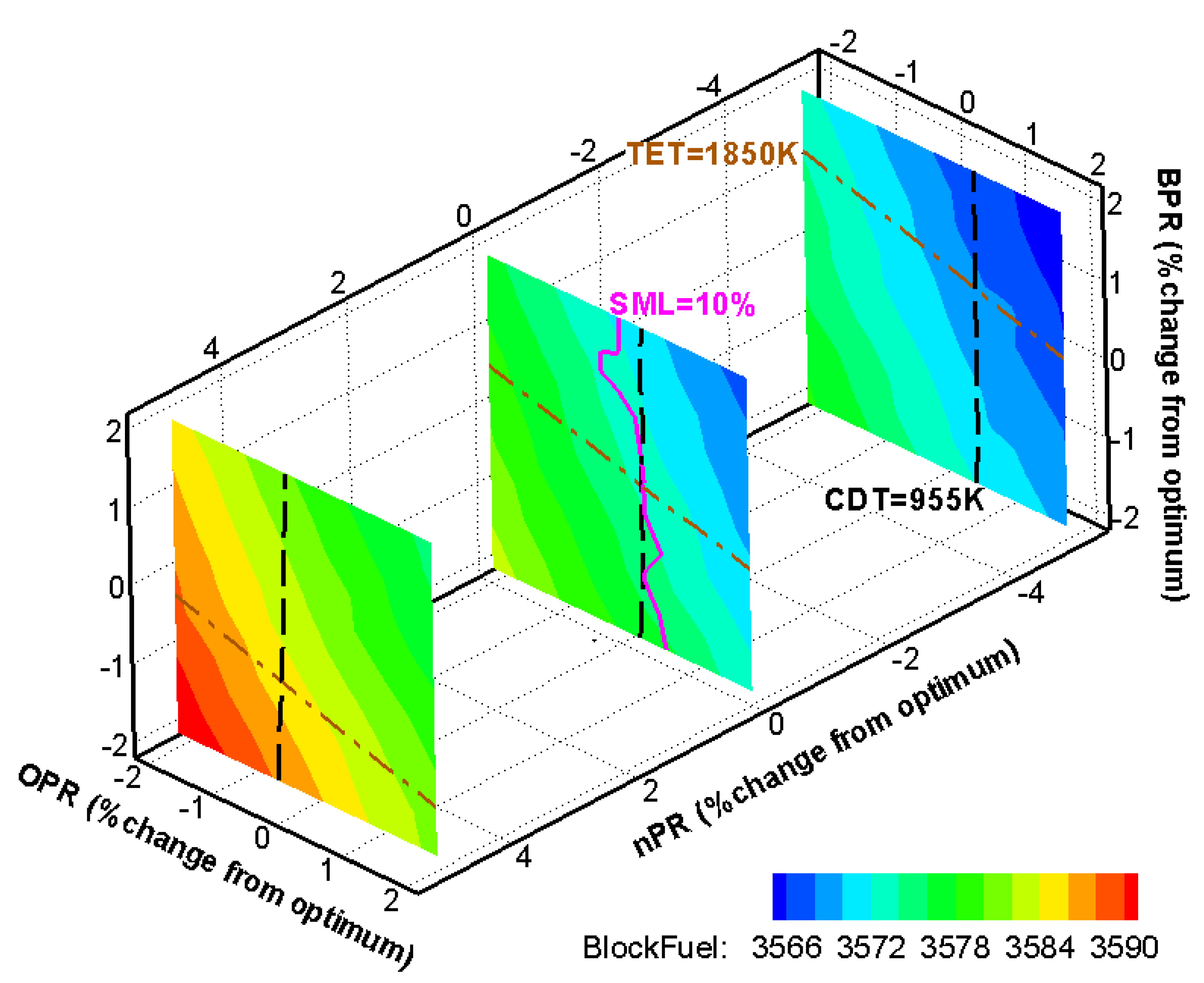
3.5. Optimization Results

A three-step optimization approach is implemented [7], with the Adaptive Simulated Annealing technique [61] being used as a first step to explore the entire design space and identify the global optimal design location, followed by a Downhill Simplex method [62] to refine its exact location and finally a design-of-experiments around it to confirm and visualize it.
The compressor design performance for the fuel burn optimal solution is listed in Table 3. Figure 7 presents the design space around the optimal values of N s t g and U 1 , t , for the HP compressor. Compressor efficiency (eff) and consequently fuel burn (FB) improve with decreasing U 1 , t and N s t g . However, the transient surge margin limit precludes altogether the nine-stage solution and the lower range of U 1 , t values for the ten-stage option. The LP compressor design space exhibits a similar behavior.
For the compressor design choices in this test case, the work distribution is established by reaching the limits on the stator hub diffusion factor for the first three stages of both LPC and HPC and the rotor tip diffusion factor for all other stages.
Although HP and LP turbine aerodynamic design parameters are not included in this example as optimization variables, the calculated turbine stage and overall design efficiencies are affected according to the flow conditions established from varying the cycle and compressor design parameters, including changes in cooling flows. Off-design performance is influenced by the turbine map scaling and the matching with the compressor that has a new map in every design loop. Thus, the optimal fuel burn solution directly includes the influence of the turbine aero-thermodynamic design choices.
Figure 8 shows three high-power (top-of-climb, mid-cruise and rolling take-off) and three low-power (ground idle, descent idle at top-of-descent conditions and approach idle at bottom-of-descent conditions) operating points on the LPC (plot a) and HPC (plot b) maps. These are the maps generated by MLAC for the design produced by MLDC, used in the engine model for the design and off-design steady-state and transient simulations. For the HPC, the steady state surge margin is greater than 22% for all points but the ground idle one, where it drops to 19%. The LPC surge margin is also higher than 21% for the high-power conditions and descent idle, stays above 12% for the approach idle and drops down to 6% at ground idle. This may not be adequate for decelerating to ground idle conditions and indicates that an additional constraint may have had to be imposed, e.g., in the form of response and operability requirements for a transient maneuver to and from ground idle conditions. It should be noted that in this test case idle thrust is <4% of the rated take-off SLS thrust.
The fuel-burn optimal values of the engine design parameters (at ToC) are included in Table 4. This solution gives a fuel burn of 3574 kg which is approximately 9.5% lower compared to the same mission executed with a current technology engine, e.g., similar to a geared turbofan of EIS-2016. Further improvement is constrained by the limits of 1850 K on TET, 955 K on CDT and the transient surge margins of LPC (SML = 10%) and HPC (SMH = 14%). This can be observed in Figure 9 and Figure 10, where FB contour plots for different combinations of design parameters are depicted.
Specifically, Figure 9 shows that lower FB can be obtained by increasing both BPR and OPR and reducing nPR (i.e., higher loaded HPC). However, BPR and OPR increases are prevented by the TET and CDT limits, respectively, while, for the lower nPR case, SMH is below 7% throughout the entire BPR-OPR design space. Even for the optimum nPR case, the HPC and LPC transient surge margin limits would have prevented further FB improvement even if the temperature limits were allowed to be higher. This is also the case when considering the variation of FPR and sFN around their optimal values, as shown in Figure 10. The intersection of SML and SMH limit lines define the valid design space area, which reduces significantly as sFN increases.
For the optimal solution, Figure 11 shows the transient maneuver operating line on the LPC (plot a) and HPC (plot b) maps. The variation of surge margin with time is also included as an insert in both plots and demonstrates that the solution is constrained by the limits imposed on these parameters. Both the acceleration and deceleration response requirements are met with a thrust margin of just over 1 kN (Figure 11c).
To examine if the transient simulation included in the engine design optimization is a representative one for assessing response and operability, three additional transient maneuvers are performed for the optimal engine-design case. The first one is a square cycle at top-of-descent conditions (MNf = 0.76, ALT = 10,668 m) between descent idle ( F N i d l e ) and top-of-climb ( F N m a x ) operating settings. For this case, the acceleration and deceleration response requirements are both set to 15 s, for reaching 95% of F N m a x and 95% thrust decay, respectively, for the same compressor surge margin limits as for the certification maneuver. The results of this simulation are shown in Figure 12 and confirm that both performance requirements and compressor stability limits are respected. It should be pointed out that at these conditions, F N i d l e is negative since momentum drag is higher than total gross thrust.
The second maneuver is an acceleration at bottom-of-descent conditions (MNf = 0.30, ALT = 1524 m) from descent idle to top-of-climb operating settings with a response requirement of 8 s to 95% of F N m a x . The HPC surge margin is only relevant in this case. The results of this simulation are shown in Figure 13. During this maneuver, the HPC surge margin remains above the 14% limit while it takes ~7 s to reach 95% of F N m a x .
The final maneuver examined is a square cycle between static seal-level ground idle and rolling take-off conditions (MNf = 0.25, ΔTISA = 15 K). The rates of acceleration and deceleration are set according to the LPC map limits. The requirements are for LPC surge margin to be greater than 0 during deceleration and LPC pressure ratio greater than 1 during acceleration. The latter is simply a numerical limit as the model will not converge for compressor PR < 1. Figure 14 shows that the engine requires less than 10 s to accelerate to 90% of RTO thrust with the HPC surge margin staying above 10%. It should be noted that the fan reaches 50% of its take-off speed in less than 3 s when the minimum requirement is that it should be less than 8 s. On the other hand, with the LPC surge margin consumed, it takes 15 s to reach 90% thrust decay, which may not be acceptable in case of a rejected take-off situation. This clearly demonstrates that such a critical transient maneuver should also be included in the overall engine design optimization scheme, in addition to the certification one, with LPC IGV and handling bleed schedules as extra design variables.
In case the transient maneuver is not included in the overall optimization loop and no constraints are imposed regarding steady-state idle performance, such as surge margin (Case-2), then a solution is produced that requires 18 kg (0.5%) less fuel to complete the mission compared to the optimization scheme that includes the transient module (Case-1). This is achieved mainly by increasing OPR by 1.2% and shifting more work to the LP compressor, by increasing nPR by 4.3%, compared to Case-1 optimal values. Further OPR increase is prevented by the CDT limit. In terms of HPC and LPC design, the optimization gives lower U 1 , t values (390 and 334 m/s, respectively) for the same number of stages, leading to slightly higher design point efficiencies (91.9% and 91.7%, respectively) in relation to Case-1 (see Table 3). The entire HPC operating line (Figure 15a) is shifted closer to the surge line, leaving a surge margin of 11.4% at ground idle conditions. Simulating the transient certification maneuver for this engine design fails to meet the operability constraints regarding compressor surge margin; see Figure 15b and compare with Figure 11b. These results clearly demonstrate the need to integrate transient analysis in the overall engine design optimization loop.

4. Conclusions

The development of a robust, flexible and fast execution module for compressor mean-line design and its integration in an overall engine preliminary design framework have been presented. The module allows compressor geometrical and flow parameters to be specified as design and constraint variables, when optimizing an engine for performance and operability. It is directly compatible with the corresponding compressor mean-line analysis module, thus ensuring a consistent and numerically stable map generation process. The maps produced can then be used in a relevant engine model to assess steady-state and transient performance. Thus, a simulation chain can be established combining compressor, engine and aircraft mission analysis modules.
For the case of a UHBR engine design optimization, it is demonstrated how compressor design influences engine response and operability and that transient performance must be accounted for simultaneously with the engine aero-thermodynamic and structural requirements and constraints, in order to correctly define the feasible design space.
For the specific test case and based on the design choices and assumptions made, it was shown that during deceleration to ground idle conditions, the operation of low pressure compressor is critical, in terms of engine operability and response.
The results were obtained considering only shaft dynamic effects (spool inertias), and this is deemed sufficient for preliminary design studies. However, it is acknowledged that there are other dynamic effects (e.g., heat soakage, tip clearance, volume dynamics, sensors and actuators lags and delays) that should be accounted for in order to have a more realistic assessment of engine response and operability. The tool developed is capable of including these effects and the authors plan to examine their influence in further studies.
The development and integration of turbine mean line design and analysis modules in the engine design framework, in a way similar to the compressor ones, is currently under way in order to further improve the fidelity of the calculations.
The modular nature of the framework allows engine and/or aircraft (e.g., oil, fuel, environmental control) sub-systems as well as engine figures of merit related to other disciplines (e.g., noise, emissions, lifing, maintenance, economics), at different levels of fidelity, to be easily integrated, thus enabling multi-objective design calculations. We plan to report such capabilities in future publications.

Author Contributions

Conceptualization, A.A., I.K. and N.A.; methodology, A.A., I.K. and N.A.; software, A.A., I.K. and N.A.; validation, A.A. and I.K.; formal analysis, A.A. and I.K.; investigation, A.A. and I.K.; data curation, A.A. and I.K.; writing—original draft preparation, A.A. and I.K.; writing—review and editing, A.A., I.K., N.A. and K.M.; visualization, A.A. and I.K.; supervision, N.A. and K.M. All authors have read and agreed to the published version of the manuscript.

Funding

This project has received funding from the Clean Sky 2 Joint Undertaking (JU) under grant agreement No 886840. The JU receives support from the European Union’s Horizon 2020 research and innovation programme and the Clean Sky 2 JU members other than the Union.

Data Availability Statement

The data presented in this study are available on request from the corresponding author.

Conflicts of Interest

The authors declare no conflict of interest.

Nomenclature

Abbreviations
0/1/2/3D0-/1-/2-/3-Dimensional
AIDLApproach Idle
BC4British C-4
BRMBlade Row Module
CFDComputational Fluid Dynamics
DCADouble Circular Arc
DIDLDescent Idle
ECSEnvironmental Control System
EISEntry Into Service
GEGeneral Electric
GIDLGround Idle
HPHigh-Pressure
HPCHigh-Pressure Compressor
HPTHigh-Pressure Turbine
IGVsInlet Guide Vanes
ISAInternational Standard Atmosphere
IVMInter-Volume Module
LPLow-Pressure
LPCLow-Pressure Compressor
MCRMid-Cruise
MLACMean-Line Analysis Code
MLDCMean-Line Design Code
NASANational Aeronautics and Space Administration
PROOSISPropulsion Object Oriented SImulation Software
RTORolling Take-Off
TLARTop Level Aircraft Requirements
ToCTop-of-Climb
UHBRUltra-High Bypass Ratio
Symbols
1/2Blade row inlet/outlet
2/3Inter-volume inlet/outlet
a Absolute flow angle (o)
a/cRelative position of max. camber (-)
A L T Altitude
A R Blade aspect ratio (-)
A V D R A V D R = ( ρ s V x ) 2 / ( ρ s V x ) 1
B P R Bypass ratio (-)
c p Static pressure rise coefficient (-)
C D T Compressor discharge temperature (K)
D F Fan diameter (m)
D F Diffusion factor (-)
D F e q Equivalent diffusion factor (-)
F N Net thrust (N)
F P R Fan pressure ratio (-)
h Height (m)
i Incidence angle (o)
I Index
j Stage number (-)
k Blade row number (-)
k s / c Relative surface roughness (-)
m ˙ Mass flow rate (kg/s)
M Mach number (-)
M N f Flight Mach number (-)
N b r Number of blade rows (-)
N s t g Number of stages (-)
N m e c h Rotational speed (rpm)
n P R Pressure ratio split parameter
n P R = log ( P t 25 / P t 2 ) log ( O P R )
O P R Overall pressure ratio
p Pressure (Pa)
P W X Customer power extraction (W)
r Radial coordinate (m)
R Radius (m)
R e Chord-wise Reynolds number (-)
s Blade row pitch length (m)
s F N Specific thrust (m/s)
t / c Relative max. thickness (-)
T Temperature (K)
T E T Turbine entry temperature (K)
U 1 , t 1st Rotor tip speed (m/s)
V Absolute flow velocity (m/s)
W Relative flow velocity (m/s)
W E C S Environmental Control System mass flow rate (kg/s)
y y = ( j 1 ) / ( N s t g 1 )
β Relative flow angle (o)
δ Deviation angle (o)
δ c Radial clearance (m)
θ Blade camber angle (o)
κ Metal angle w.r.t. axial direction (o)
Π Compressor pressure ratio (-)
ρ Flow density (kg/m3)
σ Blade row solidity (-)
ω Total pressure loss coefficient (-)
Subscripts
1/2Blade row inlet/outlet
2/3Inter-volume inlet/outlet
h Flowpath hub
i n Compressor inlet
i s Isentropic conditions
m Flowpath mean
m a x Maximum
m i n Minimum
o u t Compressor exit
r Relative frame of reference
R Rotor
s t a l l Stall conditions
S Stator
t Flowpath tip
T E Trailing edge
x Axial direction
θ Peripheral direction
Superscripts
0Total (stagnation) flow properties
s Static flow properties

Appendix A. MLDC Calculation Options

In the following, the approach to describe axial velocity, rotor inlet absolute flow angle, aspect ratio and solidity are presented. Note that the default values mentioned below were obtained by analyzing the NASA/GE E3 HPC [40]. It is known that the design of this compressor incorporated existing knowledge and experience in an optimal way for achieving top performances, and can thus be considered as an exemplary approach for compressor design purpose. The user of MLDC can modify them in a compressor design study.
The axial velocity across the compressor can be described on the basis of one of the following alternative ways:
  • Axial velocity distribution between the values at compressor inlet and exit using a user-defined parameter (VCLICO) that describes the shape of a parabola in relation to a straight line:
V x , 1 = A ( k 1 ) 2 + B ( k 1 ) + V x , i n A = 2 ( V x , i n + V x , o u t ) ( V C L I C O 1 ) ( N b r 1 ) 2 B = 3 V x , o u t + V x , i n 2 V C L I C O ( V x , i n + V x , o u t ) N b r 1 + 4 N b r ( V x , i n + V x , o u t ) ( V C L I C O 1 ) ( N b r 1 ) 2
where V x , 1 is the axial velocity at the blade row inlet, and the default value for V C L I C O is V C L I C O = 1.0 ;
2.
Specifying the coefficients of a 4th order polynomial that describes the axial velocity distribution at the inlet of the rotors (Vx,R,1) in relation to a user-defined reference value ( V ¯ x ):
V x , R , 1 V ¯ x = A V y 4 + B V y 3 + C V y 2 + D V y + 1
where the default values for the coefficients are
A V = 1.237 ,   B V = 3.251 ,   C V = 2.300 ,   D V = 0.389
3.
Using Equation (A1) but, this time, to describe the axial velocity variation between the values of the first and last stage rotor inlets.
The axial velocities at the compressor inlet ( V x , i n ) and exit ( V x , o u t ) are specified either by imposing them directly or by specifying the axial flow Mach number while, for the case of the compressor inlet, imposing the specific flow is a third option. Note that, for options 2 and 3, velocity ratios are also specified for describing the change in axial velocity between the (i) rotor outlet/inlet (default value = 0.914), (ii) stator outlet/inlet (default value = 0.980), (iii) IGVs outlet/inlet (default value = 1.078), (iv) rotor inlet/IGVs inlet (default value = 1.160), and (v) rotor inlet/stator inlet (default value = 1.050).
The rotor inlet absolute flow angle can be a user input in every stage, or can be described by specifying the coefficients of a 3rd order polynomial in relation to a user-defined reference value ( a ¯ ):
a R , 1 a ¯ = A a y 3 + B a y 2 + C a y + D a
where the default values for the coefficients are
A a = 1.806 ,   B a = 4.463 ,   C a = 2.854 ,   D a = 0.642
In order to estimate the blade chord at the mean-line, the aspect ratio is required. This is either a user input or is given as a rate of change ( δ A R ) for rotors and stators from their first stage value ( A R 1 ) and down to a user-specified minimum value ( A R m i n ):
A R j = max [ A R 1 + ( j 1 ) δ A R , A R m i n ]
where the default value for A R m i n is 1.0.
To estimate the blade count, the blade row solidity can either be a user input in every blade row, or can be estimated based on the relative tip Mach number ( M r , t , 1 ) for rotors ( σ R ) and the blade absolute flow turning ( δ a ) for stators ( σ S ) [43]:
σ R = R ¯ t R ¯ m ( 0.5 M r , t , 1 + 0.7 ) , σ S = R ¯ h R ¯ m { ( 0.0206 δ a + 0.794 ) , δ a < 44 ° ( 0.080 δ a 1.82 ) , 44 ° δ a < 60 ° 3.0 , δ a 60 °
In the above, R ¯ h and R ¯ t is the blade row average hub and tip radius, respectively, and δ a = a 1 a 2 is the absolute flow turning.

Appendix B. MLDC Available Loss and Deviation Models

A summary of the available loss and deviation correlations in MLDC is given in Table A1. Note that these correlations were made fully tunable through the introduction of appropriate scalars, the value of which can be the default one, a user input, or established numerically to match an available performance. As can be seen from Table A1, the user can select between different models, while an option for introducing customized models was also foreseen in the code.
Table A1. Summary of loss and deviation models available in MLDC.
CorrelationModelFunctional FormRefs
Design incidenceLieblein i * = f ( θ , σ , β 1 , t / c ) [36]
Herrig (default) i * = f ( θ , σ , β 1 , t / c , a / c )
Design deviationLieblein (default) δ * = f ( θ , σ , β 1 , t / c ) [36]
Howell δ * = f ( θ , σ , β 1 , t / c , a / c )
Minimum loss incidenceAungier i m i n = f ( M r , 1 , θ , i * ) [36]
Off-design deviationLieblein δ = f ( σ , β 1 , i ,   A V D R ) [36,63]
Swan (default) δ = f ( M r , 1 , D F e q ) [64]
Banjac et al. (default for IGVs) δ = f ( M 1 , θ , σ , γ , A V D R , t / c ) [65]
Endwall lossHowell (default) ω e w = f ( σ , β 1 , β 2 , A R ) [36]
Vavra ω e w = f ( σ , β 1 , β 2 , A R ) [66]
Secondary lossHowell ω s c = f ( σ , β 1 , β 2 ) [36]
Vavra ω s c = f ( σ , β 1 , β 2 , h ¯ / s , h ¯ / δ c ) [66]
Clearance lossLakshminarayana ω c l = f ( σ , β 1 , β 2 , A R , δ c / s ) [67]
Vavra ω c l = f ( σ , β 1 , β 2 , h ¯ / δ c ) [66]
Shock lossDixon et al. (default) ω s h = f ( σ , β 1 , β 2 , M r , 1 ) [68]
Steinke et al. ω s h = f ( σ , β 1 , β 2 , M r , 1 ) [69]
Reynolds number effectsAungier a R e = f ( R e ) [36]
Wright et al. s R e = f ( R e ) [70]
Koch et al. s R e = f ( R e , k s / c ) [71]
Mach number effectsAungier (default) a M a , s M a = f ( M r , 1 , W 1 , β 1 , β 2 , i , θ , σ ) [36]
Design profile lossAungier 1 (default) ω p r * = f ( σ , β 2 , D F ) [36]
Aungier ω p r * = a M a + s M a s R e [ a R e + f ( σ , β 1 , β 2 , D F e q ) ]
Off-minimum profile lossAungier (default) ω p r = ω p r * f ( i i m i n ) [36]
Blockage factorGlassman et al. (default)N/A[33,72]
Overall lossN/A ω = ω p r + ω s h + ω s c + ω e w + ω c l
Banjac et al. (default for IGVs) ω = f ( M 1 , θ , σ , γ , t / c ) [65]
1 Presumably accounts for secondary losses and Reynolds number effects too and, therefore, these are deactivated when this calculation option is selected.

References

  1. International Coordinating Council of Aerospace Industries Associations (ICCAIA). Advancing Technology Opportunities to Further Reduce CO2 Emissions in Climate Change Mitigation: Technology and Operations in ICAO 2019 Environmental Report Aviation and Environment; ICAO: Montreal, QC, Canada, 2019; Chapter 4; pp. 116–121. [Google Scholar]
  2. IATA. Aircraft Technology: Net Zero Roadmap. 2023. Available online: https://www.iata.org/contentassets/8d19e716636a47c184e7221c77563c93/aircraft-technology-net-zero-roadmap.pdf (accessed on 22 June 2023).
  3. Jones, S.M.; Haller, W.J.; Tong, M.T. An N+3 Technology Level Reference Propulsion System; NASA Technical Memorandum; TM–2017–219501; NASA Glenn Research Center: Cleveland, OH, USA, 2017.
  4. Csank, J.T.; Thomas, G.L. Dynamic Analysis for a Geared Turbofan Engine with Variable Area Fan Nozzle. In Proceedings of the 53rd AIAA/SAE/ASEE Joint Propulsion Conference, AIAA 2017-4819, Atlanta, GA, USA, 10–12 July 2017. [Google Scholar] [CrossRef]
  5. Electronic Code of Federal Regulations. Available online: https://www.ecfr.gov/cgi-bin/text-idx?SID=aa3a99819fbf162f142eee0ec759f8df&mc=true&node=se14.1.33_173&rgn=div8 (accessed on 22 June 2023).
  6. Vieweg, M.; Wolters, F.; Reitenbach, S.; Hollmann, C.; Becker, R.-G. Multi-Disciplinary Tool Coupling for the Determination of Turbofan Transients During Preliminary Design. In Proceedings of the ASME Turbo Expo 2019, Phoenix, AZ, USA, 17–21 June 2019. [Google Scholar] [CrossRef]
  7. Alexiou, A.; Aretakis, N.; Kolias, I.; Mathioudakis, K. Novel Aero-Engine Multi-Disciplinary Preliminary Design Optimization Framework Accounting for Dynamic System Operation and Aircraft Mission Performance. Aerospace 2021, 8, 49. [Google Scholar] [CrossRef]
  8. Gallimore, S.J. Axial Flow Compressor Design. Proc. Inst. Mech. Eng. Part C J. Mech. Eng. Sci. 1999, 213, 437–449. [Google Scholar] [CrossRef]
  9. Kolias, I.; Alexiou, A.; Aretakis, N.; Mathioudakis, K. Axial Compressor Mean-Line Analysis: Chocking Modelling and Fully-Coupled Integration in Engine Performance Simulations. Int. J. Turbomach. Propuls. Power 2021, 6, 4. [Google Scholar] [CrossRef]
  10. Kiss, A.; Spakovszky, Z. Effects of Transient Heat Transfer on Compressor Stability. In Proceedings of the ASME Turbo Expo 2018, Oslo, Norway, 11–15 June 2018. [Google Scholar] [CrossRef]
  11. Neumann, N.; Peitsch, D. Introduction and Validation of a Mean Line Solver for Present and Future Turbomachines. In Proceedings of the 24th ISABE Conference, Canberra, Australia, 22–27 September 2019. ISABE-2019-24441. [Google Scholar]
  12. Vidal, L.E.F.; Pachidis, V.; Tunstall, R.J. Generating Axial Compressor Maps to Zero Speed. Proc. Inst. Mech. Eng. Part A J. Power Energy 2021, 235, 956–973. [Google Scholar] [CrossRef]
  13. Zhang, Y.; Zhang, S.; Xiao, Y. Aerodynamic Performance Prediction of Transonic Axial Multistage Compressors Based on One-Dimensional Meanline Method. In Proceedings of the ASME Turbo Expo 2020, Virtual, 21–25 September 2020. [Google Scholar] [CrossRef]
  14. Jones, S.M. Design of an Object-Oriented Turbomachinery Analysis Code: Initial Results. In Proceedings of the 22nd ISABE Conference, Phoenix, AX, USA, 25–30 October 2015. ISABE-2015-20015. [Google Scholar]
  15. Madadi, A.; Benisi, A.H. Performance Predicting Modeling of Axial-Flow Compressor at Design and Off-Design Conditions. In Proceedings of the ASME Turbo Expo 2008, Berlin, Germany, 9–13 June 2008. [Google Scholar] [CrossRef]
  16. Zhang, X.; Ju, Y.; Zhang, C. Accuracy and Sensitivity Analysis of Aerodynamic Performance Prediction Models for Transonic Axial-Flow Compressors. In Proceedings of the ASME Turbo Expo 2020, Virtual, 21–25 September 2020. [Google Scholar] [CrossRef]
  17. Zhang, Y.; Zhang, S. Performance Prediction of Transonic Axial Multistage Compressor Based on One-Dimensional Meanline Method. Proc. Inst. Mech. Eng. Part A J. Power Energy 2021, 235, 1355–1369. [Google Scholar] [CrossRef]
  18. Mattingly, J.D.; Heiser, W.H.; Pratt, D.T. Aircraft Engine Design, 2nd ed.; AIAA Education Series: Reston, VA, USA, 2002; ISBN 1-56347-538-3. [Google Scholar]
  19. Mattingly, J.D. Elements of Gas Turbine Propulsion; AIAA Education Series: Reston, VA, USA, 2005; ISBN -10 1-56-347778-5. [Google Scholar]
  20. Turner, M.G.; Merchant, A.; Bruna, D. A Turbomachinery Design Tool for Teaching Design Concepts for Axial-Flow Fans, Compressors, and Turbines. In Proceedings of the ASME Turbo Expo 2006, Barcelona, Spain, 8–11 May 2006. [Google Scholar] [CrossRef]
  21. Bruna, D.; Cravero, C.; Turner, M.G.; Merchant, A. An Educational Software Suite for Teaching Design Strategies for Multistage Axial Flow Compressors. In Proceedings of the ASME Turbo Expo 2007, Montreal, QC, Canada, 14–17 May 2007. [Google Scholar] [CrossRef]
  22. Turner, M.G.; Merchant, A.; Bruna, D. Applications of a Turbomachinery Design Tool for Compressors and Turbines. In Proceedings of the 43rd AIAA Joint Propulsion Conference and Exhibit, Cincinnati, OH, USA, 8–11 July 2007. [Google Scholar] [CrossRef]
  23. Turner, M.G.; Park, K.; Siddappaji, K.; Dey, S.; Gutzwiller, D.P.; Merchant, A.; Bruna, D. Framework for Multidisciplinary Optimization of Turbomachinery. In Proceedings of the ASME Turbo Expo 2010, Glasgow, UK, 14–18 June 2010. [Google Scholar] [CrossRef]
  24. Tomita, J.T.; Barbosa, J.R. Numerical Tools for High Performance Axial Compressor Design for Teaching Purpose. In Proceedings of the ASME Turbo Expo 2012, Copenhagen, Denmark, 11–15 June 2012. [Google Scholar] [CrossRef]
  25. Denton, J.D. MULTALL-An Open Source, CFD Based, Turbomachinery Design System. In Proceedings of the ASME Turbo Expo 2017, Charlotte, NC, USA, 26–30 June 2017. [Google Scholar] [CrossRef]
  26. Veres, J.P. Axial and Centrifugal Compressor Mean Line Flow Analysis Method. In Proceedings of the 47th AIAA Aerospace Sciences Meeting, Orlando, FL, USA, 5–8 January 2009. [Google Scholar] [CrossRef]
  27. Becker, R.-G.; Reitenbach, S.; Klein, C.; Otten, T.; Nauroz, M.; Siggel, M. An Integrated Method for Propulsion System Conceptual Design. In Proceedings of the ASME Turbo Expo 2015, Montreal, Canada, 15–19 June 2015. [Google Scholar] [CrossRef]
  28. Banjac, M.; Petrovic, M.V. Development of Method and Computer Program for Multistage Axial Compressor Design: Part I-Mean Line Design and Example Cases. In Proceedings of the ASME Turbo Expo 2018, Oslo, Norway, 11–15 June 2018. [Google Scholar] [CrossRef]
  29. He, Y.; Sun, J.; Song, P.; Wang, X.; Xu, D. Development of a Multi-Objective Preliminary Design Optimization Approach for Axial Flow Compressors. In Proceedings of the ASME Turbo Expo 2018, Oslo, Norway, 11–15 June 2018. [Google Scholar] [CrossRef]
  30. Lei, F.; Ju, Y.; Zhang, C. A Rapid and Automatic Optimal Design Method for Six-Stage Axial-Flow Industry Compressor. J. Therm. Sci. 2021, 30, 1658–1673. [Google Scholar] [CrossRef]
  31. Lei, F.; Zhang, C. Preliminary Optimization of Multi-Stage Axial-Flow Industrial Process Compressors Using Aero-Engine Compressor Design Strategy. Appl. Sci. 2021, 11, 9248. [Google Scholar] [CrossRef]
  32. Kaden, W.; Turner, M.G. Open Source Axial Compressor Mean-Line Design Tool for Supercritical Carbon Dioxide. In Proceedings of the ASME Turbo Expo 2021, Virtual, 7–11 June 2021; GT2021-59961. [Google Scholar] [CrossRef]
  33. Glassman, A.J.; Lavelle, T.M. Enhanced Capabilities and Modified Users Manual for Axial-Flow Compressor Conceptual Design Code CSPAN; NASA TM-106833; NASA Lewis Research Center: Cleveland, OH, USA, 1995.
  34. Walsh, P.P.; Fletcher, P. Gas Turbine Performance, 2nd ed.; ASME Press: New York, NY, USA, 2004; ISBN 0-632-06434-X. [Google Scholar]
  35. Saravanamuttoo, H.I.H.; Rogers, G.F.C.; Cohen, H.; Straznicky, P.V.; Nix, A.C. Gas Turbine Theory, 7th ed.; Pearson: Harlow, UK, 2017; ISBN 9781-292-09309-3. [Google Scholar]
  36. Aungier, R.H. Axial-Flow Compressors, A Strategy for Aerodynamic Design and Analysis, 1st ed.; ASME: New York, NY, USA, 2003; ISBN 0-7918-0192-6. [Google Scholar]
  37. Miller, D.C.; Wasdell, D.L. Off-Design Prediction of Compressor Blade Losses. Proc. IMechE 1987, C279/87, 249–260. [Google Scholar]
  38. Banjac, M.; Petrovic, M.V.; Wiedermann, A. Secondary Flows, Endwall Effects, and Stall Detection in Axial Compressors. J. Turbomach. 2015, 137, 051004. [Google Scholar] [CrossRef]
  39. Schweitzer, J.K.; Garberoglio, J.E. Maximum Loading Capability of Axial Flow Compressors. J. Aircr. 1984, 21, 593–600. [Google Scholar] [CrossRef]
  40. Holloway, P.R.; Knight, G.L.; Koch, C.C.; Shaffer, S.J. Energy Efficient Engine: High Pressure Compressor Detail Design Report; NASA, CR-165558; NASA Lewis Research Center: Cleveland, OH, USA, 1982.
  41. Cline, S.J.; Fesler, W.; Liu, H.S.; Lovell, R.C.; Shaffer, S.J. Energy Efficient Engine: High Pressure Compressor Component Performance Report; NASA, CR-168245; NASA Lewis Research Center: Cleveland, OH, USA, 1983.
  42. Alexiou, A.; Aretakis, N.; Roumeliotis, I.; Kolias, I.; Mathioudakis, K. Performance Modelling of an Ultra-High Bypass Ratio Geared Turbofan. In Proceedings of the 23rd ISABE Conference, Manchester, UK, 3–8 September 2017. ISABE-2017-22512. [Google Scholar]
  43. Kolias, I.; Alexiou, A.; Aretakis, N.; Mathioudakis, K. Direct Integration of Axial Turbomachinery Preliminary Aerodynamic Design Calculations in Engine Performance Component Models. In Proceedings of the ASME Turbo Expo 2018, Oslo, Norway, 11–15 June 2018. [Google Scholar] [CrossRef]
  44. Kolias, I.; Aretakis, N.; Alexiou, A.; Mathioudakis, K. A Tool for the Design of Turbomachinery Disks for an Aero-Engine Preliminary Design Framework. Aerospace 2023, 10, 460. [Google Scholar] [CrossRef]
  45. Jeschke, P.; Kurzke, J.; Schaber, R.; Riegler, C. Preliminary Gas Turbine Design Using the Multidisciplinary Design System MOPEDS. In Proceedings of the ASME Turbo Expo 2002, Amsterdam, The Netherlands, 3–6 June 2002. [Google Scholar] [CrossRef]
  46. Panchenko, Y.; Moustapha, H.; Mah, S.; Patel, K.; Dowhan, M.J.; Hall, D. Preliminary Multi-Disciplinary Optimization in Turbomachinery Design. In Proceedings of the RTO AVT Symposium, RTO-MP-089, 57/1-22, Paris, France, 22–25 April 2002. [Google Scholar]
  47. Avellán, R.; Grönstedt, T. Preliminary Design of Subsonic Transport Aircraft and Engines. In Proceedings of the 18th ISABE Conference, Beijing, China, 2–7 September 2007. ISABE-2007-1195. [Google Scholar]
  48. Bretschneider, S.; Staudacher, S.; Arago, O. Architecture of a Techno-Economic and Environmental Risk Assessment Tool Using a Multi-Modular Build Approach. In Proceedings of the 18th ISABE Conference, Beijing, China, 2–7 September 2007. ISABE-2007-1103. [Google Scholar]
  49. Ogaji, S.; Pilidis, P.; Sethi, V. Advanced Power Plant Selection: The TERA (Techno-Economic Environmental Risk Analysis) Framework. In Proceedings of the 19th ISABE Conference, Montreal, Canada, 7–11 September 2009. ISABE-2009-1115. [Google Scholar]
  50. Vieweg, M.; Reitenbach, S.; Hollmann, C.; Schnös, M.; Behrendt, T.; Krumme, A.; Otten, T.; Meier zu Ummeln, R. Collaborative Aircraft Engine Preliminary Design Using a Virtual Engine Platform, Part B: Application. In Proceedings of the AIAA Scitech 2020 Forum, AIAA-2020-0124, Orlando, FL, USA, 6–10 January 2020. [Google Scholar] [CrossRef]
  51. Kirby, M.; Mavris, D. The Environmental Design Space. In Proceedings of the 26th International Congress of the Aeronautical Sciences, ICAS-2008-4.7.3, Anchorage, AK, USA, 14–19 September 2008. [Google Scholar]
  52. Reitenbach, S.; Krumme, A.; Behrendt, T.; Schnös, M.; Schmidt, T.; Hönig, S.; Mischke, R.; Moerland, E. Design and Application of a Multi-Disciplinary Pre-Design Process for Novel Engine Concepts. In Proceedings of the ASME Turbo Expo 2018, Oslo, Norway, 11–15 June 2018. [Google Scholar] [CrossRef]
  53. GasTurb. Available online: https://www.gasturb.de/ (accessed on 22 June 2023).
  54. Gas Turbine Simulation Program. Available online: https://www.gspteam.com/ (accessed on 22 June 2023).
  55. GitHub-NASA/T-MATS. Available online: https://www.github.com/nasa/T-MATS/ (accessed on 22 June 2023).
  56. Kyprianidis, K.G.; Colmenares, Q.R.F.; Pascovici, D.S.; Ogaji, S.O.T.; Pilidis, P.; Kalfas, A.I. EVA: A Tool for Environmental Assessment of Novel Propulsion Cycles. In Proceedings of the ASME Turbo Expo 2008, Berlin, Germany, 9–13 June 2008. [Google Scholar] [CrossRef]
  57. EcosimPro. PROOSIS Modelling and Simulation Software. Available online: http://www.proosis.com/ (accessed on 22 June 2023).
  58. Felder, J.L.; Kim, H.D.; Brown, G.V.; Chu, J. An Examination of the Effect of Boundary Layer Ingestion on Turboelectric Distributed Propulsion Systems. In Proceedings of the 49th AIAA Aerosp. Sci. Meet., AIAA-2011-300, Orlando, FL, USA, 4–7 January 2011. [Google Scholar] [CrossRef]
  59. Wilcock, R.C.; Young, J.B.; Horlock, J.H. The Effect of Turbine Blade Cooling on the Cycle Efficiency of Gas Turbine Power Cycles. ASME J. Eng. Gas Turbines Power 2005, 127, 109–120. [Google Scholar] [CrossRef]
  60. Kolias, I. Development of an Integrated System for Preliminary Design of Aircraft Gas Turbines. Ph.D. Thesis, National Technical University of Athens, Athens, Greece, 2023. [Google Scholar]
  61. Ingber, L. Simulated Annealing: Practice versus Theory. J. Math. Comput. Model. 1993, 18, 29–57. [Google Scholar] [CrossRef]
  62. Nelder, J.A.; Mead, R. A simplex method for function minimization. Comput. J. 1965, 7, 308–313. [Google Scholar] [CrossRef]
  63. Cumpsty, N.A. Compressor Aerodynamics, 1st ed.; Longman: Harlow, UK, 1989; ISBN 0-582-01364-X. [Google Scholar]
  64. Swan, W.C. A Practical Method of Predicting Transonic-Compressor Performance. J. Eng. Power 1961, 83, 322–330. [Google Scholar] [CrossRef]
  65. Banjac, M.; Petrovic, M.V.; Wiedermann, A. A New Loss and Deviation Model for Axial Compressor Inlet Guide Vanes. J. Turbomach. 2014, 136, 071011. [Google Scholar] [CrossRef]
  66. Vavra, M.H. Aero-Thermodynamics and Flow in Turbomachines; Krieger: New York, NY, USA, 1974; ISBN 0-88275-189-1. [Google Scholar]
  67. Lakshminarayana, B. Methods of Predicting the Tip Clearance Effects in Axial Flow Turbomachinery. J. Basic Eng. 1970, 92, 467–480. [Google Scholar] [CrossRef]
  68. Dixon, S.L.; Hall, C.A. Fluid Mechanics and Thermodynamics of Turbomachinery, 7th ed.; Elsevier: Woburn, MA, USA, 2014; ISBN 978-0-12-415954-9. [Google Scholar]
  69. Steinke, R.J.; Crouse, J.E. Analytical Studies of Aspect Ratio and Curvature Variations for Axial-Flow-Compressor-Inlet Stages under High Loading; NASA, TN D-3959; NASA Lewis Research Center: Cleveland, OH, USA, 1967.
  70. Wright, P.I.; Miller, D.C. An Improved Compressor Performance Prediction Model. Proc. IMechE 1991, C423/028, 69–82. [Google Scholar]
  71. Koch, C.C.; Smith, L.H., Jr. Loss Sources and Magnitudes in Axial-Flow Compressors. J. Eng. Power 1976, 98. [Google Scholar] [CrossRef]
  72. Creveling, H.F.; Carmody, R.H. Axial Flow Compressor Design Computer Programs Incorporating Full Radial Equilibrium Part I –Flow Path and Radial Distribution of Energy Specified (Program II); NASA, CR-54532; NASA Lewis Research Center: Cleveland, OH, USA, 1968.
Figure 1. Blade row modelling using BRMs and IVMs.
Aerospace 10 00726 g001
Figure 2. Comparison between the actual and MLDC flowpaths for the NASA/GE E3 HPC.
Aerospace 10 00726 g002
Figure 3. Comparison between the actual and MLDC blade geometries for the NASA/GE E3 HPC: (a) Metal angle at leading edge (LE); (b) metal angle at trailing edge (TE); (c) stagger angle; (d) blade count; (e) blade axial chord; (f) blade row solidity.
Aerospace 10 00726 g003
Figure 4. Framework for the preliminary design and assessment of novel aero-engines, showing the different design and analysis modules used in the current example.
Aerospace 10 00726 g004
Figure 6. Variation of MNf and ALT with time for aircraft mission.
Aerospace 10 00726 g006
Figure 7. HP compressor design space.
Aerospace 10 00726 g007
Figure 8. Operating points on (a) LPC map and (b) HPC map.
Aerospace 10 00726 g008
Figure 9. FB contour plot for BPR, OPR, nPR with TET, CDT and SML isolines.
Aerospace 10 00726 g009
Figure 10. FB contour plot for BPR, FPR, sFN with TET, SMH and SML isolines.
Aerospace 10 00726 g010
Figure 11. Transient simulation results for certification maneuver: (a) operating line on LPC map and surge margin variation with time; (b) operating line on HPC map and surge margin variation with time; and (c) variation of thrust with time.
Aerospace 10 00726 g011aAerospace 10 00726 g011b
Figure 12. Top-of-descent idle transient simulation results: (a) operating line on LPC map and surge margin variation with time; (b) operating line on HPC map and surge margin variation with time; and (c) variation of thrust with time.
Aerospace 10 00726 g012aAerospace 10 00726 g012b
Figure 13. End-of-descent idle acceleration results: (a) operating line on HPC map and surge margin variation with time; (b) variation of thrust with time.
Aerospace 10 00726 g013
Figure 14. Ground idle transient simulation results: (a) operating line on LPC map and surge margin variation with time; (b) operating line on HPC map and surge margin variation with time; and (c) variation of thrust with time.
Aerospace 10 00726 g014
Figure 15. (a) Steady-state operating points on HPC map; (b) transient operating line on HPC map and surge margin variation with time.
Aerospace 10 00726 g015
Table 1. Aerodynamic design point data for the NASA/GE E3 HPC.
ParameterDesign Point Value
Inlet total temperature288.15 K
Inlet total pressure101,325 Pa
Rotational speed12,416.5 rpm
Inlet mass flow rate54.4 kg/s
Overall pressure ratio25.0
Table 2. Compressor design choices.
ParameterLP CompressorHP Compressor
Flowpath ShapeConstant hub diameterConstant mean diameter
Blade ProfileStators: NACA-65
Rotors: DCA
Inlet Mach Number0.40.4
Exit Mach Number0.40.3
Velocity DistributionAccording to Equation (A1) with V C L I C O = 1
Rotor inlet flow angleAccording to Equation (A3) with a ¯ = 15°
Aspect RatioIGV: 2.5 IGV: 3.8
According to Equation (A4) with
Rotor A R 1 = 1.7, δ A R = 0.07 and A R m i n   = 1
Stator   A R 1 = 2.5 δ A R = 0.15 and A R m i n = 1
SolidityCalculated-Equation (A5)
Axial gap ratio30% of axial chord
Work DistributionFrom the aerodynamic criteria with their default values
Blockage factorDefault models in Appendix B
Incidence
Deviation
Losses
Table 3. Compressor design for optimal fuel burn solution.
ParameterLP CompressorHP Compressor
Number of Stages, N s t g 510
First Rotor Tip Speed, U 1 , t (m/s)345410
Polytropic Efficiency (%)91.691.5
Pressure Ratio3.0512.75
Table 4. Optimal fuel-burn engine design parameters at Top-of-Climb.
ParameterValue
Bypass Ratio, BPR13.6
Overall Pressure Ratio, OPR49.3
Fan Pressure Ratio, FPR1.44
Specific Thrust, sFN (m/s)99.0
Pressure Ratio Split Parameter, nPR0.35
Disclaimer/Publisher’s Note: The statements, opinions and data contained in all publications are solely those of the individual author(s) and contributor(s) and not of MDPI and/or the editor(s). MDPI and/or the editor(s) disclaim responsibility for any injury to people or property resulting from any ideas, methods, instructions or products referred to in the content.

