Analysis of Flight Loads during Symmetric Aircraft Maneuvers Based on the Gradient-Enhanced Kriging Model

Abstract

The analysis of flight loads during symmetric aircraft maneuvers is an essential but computationally intensive task in aircraft design. The significant structural elastic deformation in modern aircraft further complicates this work, adding to the computational demands. Therefore, improving the analysis efficiency of flight loads during maneuvers is crucial for accelerating design interactions and shortening the development cycle. This study explores a method for analyzing flight loads in the time domain during maneuvers of elastic aircraft by introducing a database of high-precision rigid-body aerodynamic loads. Furthermore, it combines the gradient-enhanced Kriging model to efficiently predict elastic flight loads during longitudinal maneuvers. The results indicate that the proposed surrogate-based method has high fitting accuracy with significantly improved computational efficiency, providing a new approach for efficient analysis of flight loads during aircraft maneuvers.

1. Introduction

Flight loads primarily comprise aerodynamic and inertial loads, which are crucial for structural design and have a significant influence on flight safety and performance. The structural design of aircraft is often predicated on the loads in the most severe conditions, primarily determined by the maneuvering flight.

The continuous development of aviation science and technology has steadily improved aircraft maneuverability. Aircraft speed, load factors, angle of attack, and other parameters can vary significantly. Thus, the effects of aeroelasticity cannot be neglected, and the nonlinearity of aerodynamic loads becomes important. In the computation of maneuvering loads, we need multidisciplinary coupled analysis encompassing aeroelasticity, flight dynamics, fluid dynamics, and more. In addition, this analysis requires the coverage of numerous complex flight conditions and influencing factors. Traditional analysis methods of flight loads encounter challenges when balancing computational efficiency and accuracy. The aerodynamic nonlinearity during high-attitude maneuvers makes solving flight dynamic differential equations numerically inefficient and resource-intensive. Traditional methods, such as coupling finite element method software with linear/nonlinear aerodynamic analysis, are time-consuming when analyzing several flight loads in various states during maneuvers, and they cannot meet the need for rapid computations in aircraft design.

Scholars worldwide have engaged in research using numerical simulations, wind tunnel experiments, and flight tests to develop fast and accurate flight load calculation methods. Methods based on surrogate models and high-accuracy aerodynamic databases have also developed rapidly to analyze flight loads efficiently. The standard surrogate models include algebraic models [1,2], differential and integral models [3], neural networks [4,5,6,7], random forests, and Kriging models [8], among others [9]. Differential and integral models can be effectively integrated with state-space methods, such as reduced-order models obtained using the Volterra series and proper orthogonal decomposition (POD). This integration reduces the coupled fluid–structure calculations to a lower-dimensional mathematical problem involving the modal superposition of the flow field. These models predict unsteady aerodynamic forces by utilizing the evolution of predominant flow field modes. However, computational capabilities are constrained when dealing with multivariate situations, and the precision of model calculations relies on the quantity of samples. Machine learning techniques like neural networks and random forests demand extensive sample data and computational resources. The current research indicates that these methods focus on flight envelope analysis and lack comprehensive consideration for analyzing flight loads during high-attitude maneuvers.

In recent years, the Kriging method has stood out as a rapidly advancing surrogate model, progressively finding applications in aviation and aerospace. Originating from geostatistics, South African mining engineer Krige initially proposed the concept of Kriging in his 1951 master’s dissertation [10]. Then, between 1963 and 1971, French mathematician Matheron refined and developed the theory, culminating in a comprehensive mathematical framework and set of models [11]. In 1989, Professor Sacks [12] and his colleagues extended the Kriging theory into the deterministic design and analysis of computer experiments, thus presenting a practical Kriging model. Because of the groundbreaking research efforts of Professor Sacks and others, the application of the Kriging model has proliferated across various natural science domains, experiencing continuous exploration, development, and implementation in engineering sciences, particularly aviation and aerospace. The Kriging model estimates not only the unknown function but also the error in these predictions, a distinctive feature setting it apart from other surrogate models. The model demonstrates excellent nonlinear function approximation capabilities and unique error estimation functionality. The surrogate optimization algorithms based on the Kriging model have gradually been explored and applied in research endeavors such as aerodynamic optimization [13,14,15], structural optimization, and multidisciplinary optimization [16].

The Kriging model is a semi-parametric surrogate model suitable for complex nonlinear problems. The surrogate model methods are also suitable for complex nonlinear problems include machine learning methods, such as neural network model, random forest algorithm, etc. The machine learning methods avoid mathematical analysis of the model and have high computational efficiency, which can be well applied to aircraft design. The NASA Dryden Flight Research Center used flight data to determine neural network fight load models for the F/A-18 system research aircraft [17]. Haas has established the flight load model of helicopter rotor system components in high-speed maneuvering flight by using a neural network according to the load data of helicopter flight tests [18]. Wallach et al. used a neural network model to predict the aerodynamic coefficients of a general-purpose transport aircraft [19]. The neural network models have many subjective parameters, require multiple training and experiments. Due to the poor generalization ability and difficult model establishment, other supplementary methods are needed to achieve faster, convenient, and efficient modeling. He et al. established a neural network load model for aircraft wings by using stepwise regression analysis to select input parameters and Bayesian regularization method to determine the number of hidden layer neurons to improve the generalization ability of the network [20]. The random forest algorithm has accuracy and efficiency comparable to the neural network model. In addition, the random forest algorithm has the advantages of parameter interpretability and variable sensitivity analysis, and parallel algorithms can be used to improve the training speed. Li et al. [21] studied a surrogate model for flight load analysis based on random forest. Machine learning methods such as neural networks and random forests require huge sample data and computing resources.

The Kriging model has two distinct advantages over other interpolation methods and surrogate models. Firstly, the Kriging method can consider the spatial correlation characteristics of a certain point when predicting the response value of the point. According to the correlation of random variables, the information of sample points near this point is used instead of the information of all sample points. Secondly, containing both a linear regression part and a correlation part, the Kriging method has two-layer fitting of global approximation and local simulation, so it has global and local statistical characteristics and can also give error estimates of the predicted values [14]. The existing research shows that most of these interpolation methods and surrogate models focus on the analysis of flight loads at discrete state points in the flight envelope, while the analysis of flight loads changing with time in high-attitude-maneuver flight is not fully considered.

In recent years, gradient-enhanced Kriging has been developed to improve the accuracy of Kriging models. This method builds upon the traditional Kriging model [22], introducing gradient information to enhance the computational accuracy [23,24,25,26]. It exhibits robust interpolation capabilities for nonlinear problems and effectiveness in applications such as aeroelasticity optimization for aircraft and structural optimization for underwater vehicles. Lu et al. established a surrogate model of a high-aspect-ratio composite wing for static aeroelastic optimization based on the CFD/CSD coupling method and Kriging method [27]. The gradient-enhanced Kriging model shows promising prospects in the aerospace industry with substantial benefits [28]. The strengths of this method make it particularly well suited in combination with flight load analysis methods during maneuvers.

This study focuses on analyzing flight loads during high-attitude symmetric maneuvers of elastic aircraft. Initially, a high-accuracy aerodynamic database for various flight states is introduced. Subsequently, the analysis method in the time domain based on the database of elastic aircraft maneuvers is established. This method is further augmented by integrating the gradient-enhanced Kriging model for aerodynamic force prediction. Combining these approaches can realize an efficient analysis method for the flight loads of elastic aircraft during symmetric maneuvers.

2. Methodology

2.1. Analysis Method of Elastic Flight Loads

The conditions used for the analysis of flight loads during maneuvers mainly include symmetric maneuver flight, asymmetric maneuver flight, atmospheric turbulence, and gusts. The symmetric case involves the pitching maneuver, and the asymmetric cases are the rolling and yawing maneuvers. The responses, including control surface deflection and acceleration, used in the analysis of flight loads are obtained from the time history of each maneuver response.

The main critical states (severe load conditions) of interest usually have high-maneuverability characteristics. The linear aerodynamic method can be directly coupled with structural and flight dynamics equations to determine the six-degree-of-freedom acceleration and angular velocity of the elastic aircraft. The calculation is fast, but the error is large. After the elastic correction of the linear aerodynamic forces, the elastic increments of the aerodynamic coefficients and flight loads are larger than the elastic increments of nonlinear aerodynamic forces. Therefore, the maneuver loads obtained based on this calculation leads to structural overweight. To address this, the quasi-nonlinear method has been widely applied [29], which uses computational fluid dynamics (CFD) or experimental data as the benchmark nonlinear rigid-body aerodynamic loads, and the increment in aerodynamic loads caused by the structural elastic deformation is corrected using a linear aerodynamic method such as the doublet-lattice method (DLM) and the vortex lattice method (VLM), which can improve the accuracy and efficiency of elastic flight load predictions. Since linear and nonlinear aerodynamic forces come from different sources, the data dimensions are usually also different. This problem can be solved through interpolation [30]. The static aeroelastic equation in physical coordinate system is as follows [29]:

$$M_{ff}{\ddot{u}}_f+K_{ff}{u}_f-\overline{q}{Q}_{ff}{u}_f=\exists ⌊〈{\left(Q_f^s\right)}^v|{\left(u_x\right)}^v, s\in d, p, f〉\leftarrow u_x⌋+P_f$$

(1)

where subscript f refers to the structural free degrees of-freedom. $M_{ff}$, $K_{ff}$, and $Q_{ff}$ are $n_f\times n_f$ the mass matrix, stiffness matrix, and aerodynamic influence coefficient matrix (displacement-dependent), respectively ($n_f$ is the number of degrees of freedom of the structure); $u_f$ is the $n_f\times 1$ structural displacement vector; $u_x$ is the $n_x\times 1$ state vector representing the deflection of the control surfaces, aerodynamic angle, angular rate, and acceleration in six degrees of freedom; $\overline{q}$ is the dynamic pressure; $〈{\left(Q_f^s\right)}^v|{\left(u_x\right)}^v, s\in d, p, f〉$ is the $n_f\times 1$ aerodynamic forces generated by $u_x$, obtained by interpolating state variables from an external nonlinear database ($n_f$ is the number of trim variables); $d$, $p$, and $f$ are the downwash, pressure, and concentrated forces contained in the external nonlinear database, respectively; and $P_f$ is the external forces. Other state variables can be obtained by solving linear equations.

2.2. Simulation of Maneuvering Flight in the Time Domain

The analysis of flight loads during a maneuver uses the dynamics equations to determine the aircraft’s center of mass motion. The origin of the coordinate system used in the dynamics equations is at the aircraft’s center of mass, where the $x_b$-axis is parallel to the axis of the fuselage and points forward, the $z_b$-axis is in the plane of symmetry of the aircraft and points to the lower part of the fuselage, and the $y_b$-axis is determined according to the right-hand rule.

Thrust and drag are assumed to be equal, and the characteristics of the control system are not considered. Furthermore, assuming the Mach number is constant and the altitude does not vary much during the maneuver, the dynamic pressure is a function of velocity only, and the longitudinal maneuvering flight dynamics equations can be expressed as follows:

$$\left\{\begin{array}{l}m\left(\frac{\mathrm{d}{v}_{xb}}{\mathrm{d}t}+v_{zb}{\omega }_y\right)=L\sin \alpha -mg\sin \theta \\ m\left(\frac{\mathrm{d}{v}_{zb}}{\mathrm{d}t}-v_{xb}{\omega }_y\right)=-L\cos \alpha +mg\cos \theta \\ I_y\frac{\mathrm{d}{\omega }_y}{\mathrm{d}t}=M_y\end{array}\right.$$

(2)

where $v_{xb}$ and $v_{zb}$ are the components of velocity of the center of mass along the $x_b$- and $z_b$-axes, respectively; ${\omega }_y$ is the angular velocity about the $y_b$-axis; $m$ is the mass of the aircraft; $I_y$ is the moment of inertia about the $y_b$-axis; $M_y$ is the moment about the $y_b$-axis; $L$ is the lift; $\alpha$ is the angle of attack; and $\theta$ is the pitch angle. Figure 1 shows the definition of coordinate axis, angle and force in Eqution (2).

The lift and pitching moment can be expressed as follows:

$$\left\{\begin{array}{l}L=CLqs\\ M_y=C_{my}qs\overline{c}\end{array}\right.$$

(3)

where $q$ is the dynamic pressure, $s$ is the reference area, $\overline{c}$ is the reference chord length, $C_L$ is the lift coefficient, and $C_{my}$ is the pitching moment coefficient.

The relationships between $v_{xg}$, $v_{zg}$ and $v_{xb}$, $v_{zb}$ can be expressed as follows:

$$\left\{\begin{array}{l}{v}_{xg}=v_{xb}\cos \theta +v_{zb}\sin \theta \\ v_{zg}=-v_{xb}\sin \theta +v_{zb}\cos \theta \end{array}\right.$$

(4)

where $v_{xg}$ and $v_{zg}$ are the components of velocity of the center of mass along the $x_g$- and $z_g$-axes, respectively. The subscript g refers to the ground reference frame.

Since $C_L=-C_z$, the expression of $C_z$ is

$$C_z=C_{z0}+C_z^{\alpha }\alpha +C_z^{{\delta }_y}{\delta }_y+C_z^{{\omega }_y}\frac{{\omega }_y\overline{c}}{2V}$$

(5)

where ${\delta }_y$ is the rudder deflection angle, and the subscripts $x,y,z$ refer to the coordinate axes.

The expression of the pitching-moment coefficient $C_m$ is

$$C_m=C_{m0}+C_m^{\alpha }\alpha +C_m^{{\delta }_y}{\delta }_y+C_m^{{\omega }_y}\frac{{\omega }_y\overline{c}}{2V}$$

(6)

$u_x$ in Equation (1) refers to the aileron angle, angle of attack, pitch rate, and acceleration in 6 directions during symmetric aircraft maneuvers.

Using the dynamics equations and substituting the acceleration of the six degrees of freedom, angular velocity, and initial conditions, the maneuvering flight trajectory can be obtained using a direct integration method such as Runge–Kutta. The expression of the fourth-order Runge–Kutta for dynamic equation $\dot{x}=f\left(t,x\right)$ can be expressed as follows [31]:

$$\left\{\begin{array}{c}x(k+1)=x(k)+\frac{h}{6}(k_1+2k_2+2k_3+k_4)\\ x(0)=x_0\\ h=t(k+1)-t\left(k\right)\\ k_1=f\left(t(k),x(k)\right)\\ k_2=f\left(t(k)+\frac{h}{2},x(k)+\frac{h}{2}{k}_1\right)\\ k_3=f\left(t(k)+\frac{h}{2},x(k)+\frac{h}{2}{k}_2\right)\\ k_4=f\left(t(k)+h,x(k)+h{k}_3\right)\end{array}\right.$$

(7)

Pp5 Rwhere $t$ represents time, and $x$ represents state variables. For time-domain response analysis of longitudinal maneuvers, $x={\left[\begin{array}{ccccccccc}\theta & \dot{\theta }& \ddot{\theta }& u_{xg}& {\dot{u}}_{xg}& {\ddot{u}}_{xg}& u_{\mathrm{z}g}& {\dot{u}}_{zg}& {\ddot{u}}_{zg}\end{array}\right]}^T$, where θ is the pitching angle. $u_{xg}$ and $u_{yg}$ are the displacement of the center of mass motion in the ground reference frame.

Based on the flight dynamics equations and the aeroelastic equations of longitudinal maneuvers and using the Runge–Kutta method, the maneuver loads of elastic aircraft can be analyzed, and the flowchart is shown in Figure 2.

“Straight and level flight” implies the stable flight state of the aircraft, which is the initial state and end state of the maneuvering process.

• Execute flight loads analysis and aeroelastic trim: calculate the corresponding aerodynamic force distribution according to the maneuver order (deflection law of control surface) and flight parameters (e.g., angle of attack). Obtain elastically corrected maneuvering flight load data through aerodynamic/structural/aerostatic analysis.
• Perform numerical integration: use the aerodynamic parameters and flight load data at that moment and the Runge–Kutta method to solve the longitudinal dynamics equations and obtain the kinematic characteristics in maneuver flight (attitude and trajectory).
• Update attitude and trajectory: update data such as angle of attack, pitching rate, maneuvering load, flight velocity and trajectory, etc.
• Update trim condition: update maneuver instructions and flight parameters.
• Recover: check whether the attitude has corrected the maneuver. If “yes”, the maneuver process ends and returns to the straight and level flight state. If “no”, update time and proceed to the calculation of the next time step.

2.3. Theory of Gradient-Enhanced Kriging

(1)

Universal Kriging

Kriging methods are semiparametric interpolation methods that predict information at unknown sites using information from a series of sampled sites. Universal Kriging assumes the model consists of two parts [32]: a global approximation (the linear regression part) $F(x)$ and a local deviation (the nonparametric stochastic part) $Z(x)$:

$$y(x)=F(x)+Z(x)$$

(8)

The linear regression part can be expressed as

$$F(x)=f_1(x){\beta }_1+\cdots +f_p(x){\beta }_p=f{(x)}^T\mathit{\beta }$$

(9)

where $f_i(x), i=1,2,\cdots ,p$ can be a constant, linear, or quadratic polynomial. The polynomial coefficients are determined using the least-squares method, which can be viewed as an optimization problem. Assume that the function $y:{ℝ}^m\to ℝ$ is sampled at $n$ sites:

$$S=\left[\begin{array}{c}{x}^{(1)}\\ x^{(2)}\\ ⋮\\ x^{(n)}\end{array}\right]=\left[\begin{array}{cccc}{x}_1^{(1)}& x_2^{(1)}& \cdots & x_1^{(1)}\\ x_1^{(2)}& x_2^{(2)}& \cdots & x_2^{(2)}\\ ⋮& ⋮& & ⋮\\ x_1^{(n)}& x_2^{(n)}& \cdots & x_m^{(n)}\end{array}\right]\in {ℝ}^{n\times m}$$

(10)

The corresponding responses are

$$y_S={\left[\begin{array}{cccc}{y}^{(1)}& y^{(2)}& \cdots & y^{(n)}\end{array}\right]}^{\mathrm{T}}\in {ℝ}^n$$

(11)

We can predict the function at untried $x$ using the sampled datasets $\left(S,y_S\right)$.

For the stochastic component, the covariant matrix can be expressed as

$$\mathrm{Cov}\left[Z(x_i),Z(x_j)\right]={\sigma }^{2}R(x_i,x_j)$$

(12)

where ${\sigma }^2$ is the variance of $Z(x)$ and $R(x_i,x_j)$ is the spatial correlation function, which only depends on the Euclidean distance between two sites, $x_i$ and $x_j$ ($R(x_i,x_j)=1$ when $x_i$ and $x_j$ coincide, and $R(x_i,x_j)$ monotonically decreases toward 0 as the distance between $x_i$ and $x_j$ increases toward infinity).

(2)

Gradient-enhanced Kriging

GEK [8], a new surrogate modeling method developed in recent years, is an improvement on universal Kriging that utilizes gradient information to increase the model’s accuracy. Assuming that both the function value and gradient of the function $y:{ℝ}^m\to ℝ$ are evaluated at $n$ sites, the sample sites are expressed as

$$S={\left[\begin{array}{cccccccccc}{x}^{(1)}& \cdots & x^{(n)}& x^{(1)}& \cdots & x^{(1)}& \cdots & x^{(n)}& \cdots & x^{(n)}\end{array}\right]}^{\mathrm{T}}\in {ℝ}^{\left(n+nm\right)\times \left(n+nm\right)}$$

(13)

The corresponding responses and gradients are expressed as

$$y_S={\left[\begin{array}{cccc}{y}^{(1)}& y^{(2)}& \cdots & y^{(n)} \begin{array}{cccc}{\frac{\partial y}{\partial x}}^{(1)}& {\frac{\partial y}{\partial x}}^{(2)}& \cdots & {\frac{\partial y}{\partial x}}^{(n^{\prime })}\end{array}\end{array}\right]}^{\mathrm{T}}\in {ℝ}^{n+nm}$$

(14)

where ${\frac{\partial y}{\partial x}}^{(j)}={\left(\frac{\partial y}{\partial x_k}\right)}^{(j)}, k=\in 1,2,\cdots ,m, j=1,2,\cdots ,n^{\prime }$, are the gradient vectors.

The GEK predictor of function $y$ at an unknown site $x$ is expressed as a linear weighting of all sampled function values and the gradients:

$$\widehat{y}\left(x\right)={\displaystyle \sum _{i=1}^n{\omega }^{(i)}{y}^{(i)}}+{\displaystyle \sum _{i=1}^n{\lambda }^{(i)}\partial y^{(i)} }x\in {ℝ}^m$$

(15)

where ${\omega }^{(i)}$ and ${\lambda }^{(i)}$ are weighting factors. $\partial y^{(i)}={\frac{\partial y}{\partial x}}^{(i)}$ are the gradients.

Similarly to universal Kriging, the assumption of stationary random processes is introduced:

$$Y\left(x\right)={\beta }_0+Z\left(x\right)$$

(16)

where ${\beta }_0\in {ℝ}^1$ is a constant and stationary random processes $Z\left(·\right)$ have a zero mean and a covariance of

$$\left\{\begin{array}{c}\mathrm{Cov}\left[Z\left(x^{(i)}\right),Z\left(x^{(j)}\right)\right]={\sigma }^{2}R\left(x^{(i)},x^{(j)}\right)\\ \mathrm{Cov}\left[Z\left(x^{(i)}\right),\frac{\partial Z\left(x^{(j)}\right)}{\partial x_k}\right]={\sigma }^2\frac{\partial R\left(x^{(i)},x^{(j)}\right)}{\partial x_k^{(j)}}\\ \mathrm{Cov}\left[\frac{\partial Z\left(x^{(i)}\right)}{\partial x_k},Z\left(x^{(j)}\right)\right]={\sigma }^2\frac{\partial R\left(x^{(i)},x^{(j)}\right)}{\partial x_k^{(i)}}\\ \mathrm{Cov}\left[\frac{\partial Z\left(x^{(i)}\right)}{\partial x_k},\frac{\partial Z\left(x^{(j)}\right)}{\partial x_k}\right]={\sigma }^2\frac{{\partial }^{2}R\left(x^{(i)},x^{(j)}\right)}{\partial x_k^{(i)}\partial x_k^{(j)}}\end{array}\right.$$

(17)

where $\frac{\partial R\left(x^{(i)},x^{(j)}\right)}{\partial x_k^{(i)}}$, $\frac{\partial R\left(x^{(i)},x^{(j)}\right)}{\partial x_k^{(j)}}$, and $\frac{{\partial }^{2}R\left(x^{(i)},x^{(j)}\right)}{\partial x_k^{(i)}\partial x_k^{(j)}}$ are the first- and second-order partial derivatives of the spatial correlation function $R$ with respect to the kth component of $x$. $R(x_i,x_j)$ is the spatial correlation function for any two points, whose value is only related to the spatial distance, decreasing as the distance increases. $R(x_i,x_j)$ is 1 when the distance is zero and is 0 when the distance is infinity. Several options can commonly be used as spatial correlation functions (e.g., Gaussian exponential model). Since the correlation function $R$ is an explicit function of the positional variable $x_i$, it can be derived directly.

Similarly to universal Kriging, the predicted values of the GEK model can be derived as

$$\left\{\begin{array}{l}\widehat{y}\left(x\right)={\beta }_0+r^T\left(x\right)R^{-1}\left(y_S-{\beta }_{0}F\right)\\ F={\left[\begin{array}{ccc}1& \cdots & 1\begin{array}{ccc} 0& \cdots & 0\end{array}\end{array}\right]}^{\mathrm{T}}\\ {\beta }_0={\left(F^T{R}^{-1}F\right)}^{-1}{F}^T{R}^{-1}{y}_S\end{array}\right.$$

(18)

where $R$ is the correlation matrix and $r$ is the correlation vector.

The mean square error (MSE) of the predicted value can be expressed as follows:

$$\begin{array}{c}\mathrm{MSE}\left[\widehat{y}\left(x\right)\right]={\sigma }^2\left\{1.0-{\left[\begin{array}{c}r\\ 1\end{array}\right]}^T{\left[\begin{array}{cc}R& F\\ F^T& 0\end{array}\right]}^{-1}\left[\begin{array}{c}r\\ 1\end{array}\right]\right\}\\ \hspace{1em}\hspace{1em}\hspace{1em}\hspace{1em}\hspace{1em}\hspace{1em}\hspace{1em}\hspace{1em}\hspace{1em}=\left[1.0-r^T{R}^{-1}r+{\left(r^T{R}^{-1}F-1\right)}^2/\left(F^T{R}^{-1}F\right)\right]\end{array}$$

(19)

(3)

The comparison of universal Kriging and GEK for nonlinear function prediction

The function $z=f\left(x,y\right)$ can be expressed as follows:

$$z=x^2\cos \left(\frac{y^2}{4}\right)+e^{4\sin \left(x^2\right)}+20$$

(20)

Latin hypercubic sampling was used to obtain the sample sites. The function value and gradient are calculated at each sample site. The response surfaces of universal Kriging and GEK, together with the original function, are shown in Figure 3 and Figure 4. The black dots in Figure 3 and Figure 4 represent the sampling points. The MSEs of the predicted values are shown in

Table 1. MSE of the predicted value.

Number of Samples	MSE of Kriging Model	MSE of GEK Model
20	0.1549	0.0176
40	0.0559	0.0024

. Dong et al. showed that the Latin hypercube and uniform sampling methods can be used to obtain a better uniform sample space [33].

Based on the curve fitting of contour lines in the contour map, the fitted curve of GEK has a high accuracy, and its trend is very similar to that of the original function. The accuracy of the fitted curve for the original Kriging model is slightly worse, but the numerical error is small at the sampled sites. The fitting accuracy is closely related to the number of samples, where more samples yield a higher corresponding fitting accuracy.

Laurenceau et al. [26,34,35] compared the accuracy of universal Kriging, direct GEK, and indirect GEK for the prediction of aerodynamic forces, showing that both gradient-enhanced Kriging models have a higher accuracy than that of the universal Kriging model with the same number of training samples.

2.4. Analysis Method of Maneuvering Flight Loads Based on GEK Model

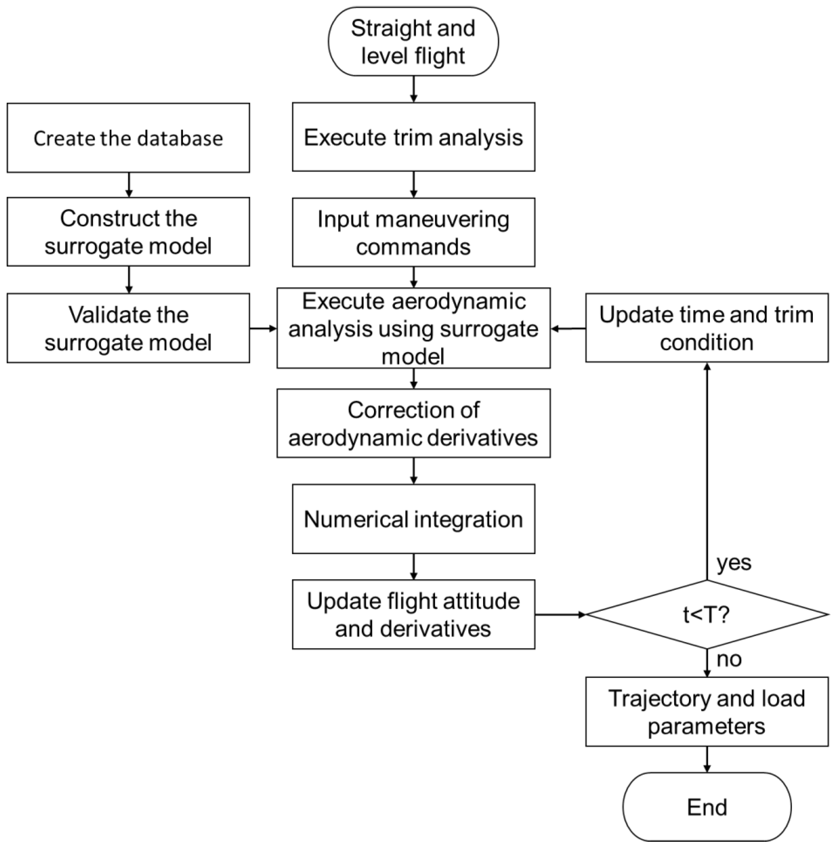
Based on elastic flight loads and the simulation of maneuvering flight in the time domain, aerodynamic derivative corrections can be solved through fast and efficient aerodynamic analysis using the GEK model. The analysis process of maneuvering flight loads based on the GEK model is summarized in the following steps, and the specific flowchart is shown in Figure 5.

• Calculate maneuvering flight loads using linear and nonlinear aerodynamic methods to obtain the range of changes in aerodynamic parameters during the maneuvers. Then, set input and output variables and prepare data for training and calibrating the model. Finally, build the surrogate model for aerodynamic analysis based on the GEK method and check its accuracy.
• Set the initial flight state as straight and level, carry out the trim analysis to obtain parameters, such as angle of attack and angular deflections of control surfaces, and set the initial values of the aerodynamic derivatives.
• Solve the input variables (maneuver commands) for the next moment according to the requirements of the maneuver and perform an aerodynamic analysis using the surrogate model.
• Solve the flight dynamics equations with elastic corrections using the Runge–Kutta method to obtain new aerodynamic derivatives.
• Update the flight attitude according to the new aerodynamic derivatives.
• Determine whether the cycle of the time step ends. If not, update the time, trim the conditions (flight attitude), update the maneuver commands, and repeat steps 3 to 6 in the next time step. If so, the flight trajectory and parameters of aerodynamic loads during the maneuvering flight are obtained.

3. Numerical Validation and Analysis

This section presents an example flight load analysis for a specific aircraft. We validate the accuracy of predicting maneuvering loads using GEK by comparing it with the aerodynamic/structural coupling results, in which we analyze the errors in the load predictions obtained by the surrogate model.

3.1. Models and Flight Conditions for Analysis

The model used for flight load analysis is a high-speed, highly maneuverable flying-wing aircraft with a takeoff weight of 20.1 tons, a wing area of 38.2 m², and a wingspan of 11.1 m. Its shape is illustrated in Figure 6. The aircraft model used in this paper has a tailless configuration. The ailerons on both sides are deflected in the same direction, acting as elevators. We define aileron deflection downward as positive.

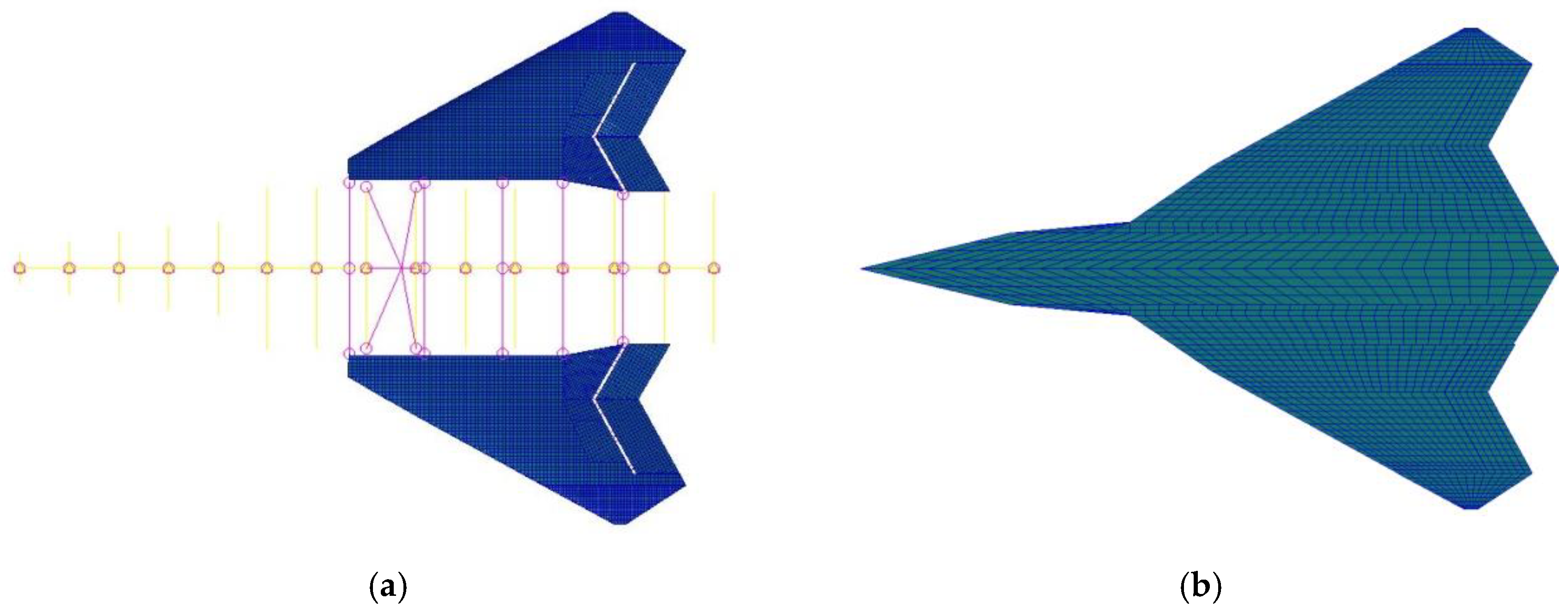
The flight load analysis is based on the static aeroelasticity module of MSC.NASTRAN. Further enhancement is achieved by integrating the Euler equations and incorporating nonlinear CFD with viscous drag correction through the MGAERO softwareV3.1. The structural mesh used in MSC.NASTRAN is a panel-bar model, the mesh number is 21,291, and the plane aerodynamic mesh number is 2114. The mesh number of the MGAERO model is 2,648,740 and the boundary conditions for subsonic and low supersonic are used. Figure 7 shows the structural finite element model and aerodynamic mesh grids of MSC.NASTRAN. Figure 8 shows the aerodynamic mesh grids of MGAERO. Combining MSC.NASTRAN and MGAERO on the flight load analysis, the aerodynamic data obtained by MGAERO are used as an external aerodynamic database and interpolated into aerodynamic mesh grids of MSC.NASTRAN. According to the data of flight conditions, Nastran performs static aeroelastic analysis by the interpolation fitting method; static aeroelastic analysis is used as a quasi-steady aerodynamic analysis method in the steady trim calculation, which can satisfy arbitrary overload conditions. The time effect is reflected by the Runge–Kutta method in the maneuvering process.

With the improvement of aircraft flight performance, the impact of the elastic deformation of aircraft structures on air flow cannot be ignored. Meanwhile, as the angle of attack and other flight parameters increase, the nonlinear characteristics of the aerodynamic force also increase greatly.

Table 2. Comparison of aerodynamic parameters and flight loads under rigid/elastic aerodynamic forces.

	N Factor	${\mathit{C}}_{\mathit{l}\mathit{\alpha }}$ (rad−1)	${\mathit{M}}_{\mathit{y}\mathit{\alpha }}$ (rad−1)	${\mathit{C}}_{\mathit{l}\mathit{\delta }}$ (rad−1)	${\mathit{M}}_{\mathit{y}\mathit{\delta }}$ (rad−1)	Shearing Force of Wing Root (kN)	Bending Moment of Wing Root (kN·m)
Rigid linear aerodynamics	9.04	−8.31 × 10−1	−3.48 × 10−2	−2.53 × 10−1	−6.00 × 10−2	451.8	63.8
Elastic linear aerodynamics	9.89	−8.66 × 10−1	−4.06 × 10−2	−1.95 × 10−1	−4.80 × 10−2	275.1	38.8
Rigid nonlinear aerodynamics	8.72	−7.86 × 10−1	−5.59 × 10−2	−1.94 × 10−1	−4.76 × 10−2	262.6	35.3
Elastic nonlinear aerodynamics	8.83	−7.70 × 10−1	−5.59 × 10−2	−1.39 × 10−1	−3.61 × 10−2	263.8	35.1

compares the results of rigid aerodynamics and elastic aerodynamics based on linear aerodynamics and nonlinear aerodynamics. The flight conditions are as follows: Ma = 0.85, flight height H = 0 km, angle of attack = 0.14 rad, aileron angle = −0.087 rad. In this case, the longitudinal overload of the aircraft is about 9g, which is already a large maneuver. It can be seen that the use of linear and nonlinear aerodynamic forces and the elastic correction of aerodynamic forces greatly affect the analysis of aerodynamic parameters and the calculation results of flight loads. According to the actual situation, the calculation results considering the effect of aeroelasticity and nonlinear aerodynamic characteristics should be more reliable. The following analysis and calculation are mainly carried out on the basis of considering the elastic aerodynamics considering aeroelasticity.

A GEK surrogate model is built using steady-state pitch and abrupt pitch as examples of common symmetrical aircraft maneuvering flight conditions.

The steady-state pitch surrogate model uses flight altitude H, Mach number Ma, and N factor n_z as input variables. The angle of attack α and aileron angle δ are chosen as output variables. In the abrupt pitch surrogate model, the flight altitude H, Mach number Ma, angle of attack α, and rudder angle δ are chosen as input variables. The N factor, pitching rate, the bending moment and shearing force of wing root, and the partial derivatives of lift coefficients and moments are chosen as output variables. Details are shown in

Table 3. Input and output variables for the steady-state pitch surrogate model.

Input Variables			Output Variables
Notation	Description	Unit	Notation	Description	Unit
H	Flight altitude	km	α	Angle of attack	rad
Ma	Mach number		δ	Aileron angle	rad
nz	N factor

and

Table 4. Input and output variables for the abrupt pitch surrogate model.

Input Variables			Output Variables
Notation	Description	Unit	Notation	Description	Unit
α	Angle of attack	rad	nz	N factor
δ	Aileron angle	rad	${\omega }_y$	Pitching rate	rad/s
			S-WR	Shearing force of wing root	kN
			BM-WR	Bending moment of wing root	kN·m
			$C_{l\alpha }$, $C_{l\delta }$	Partial derivatives of lift coefficients	rad−1
			$M_{y\alpha }$, $M_{y\delta }$	Partial derivatives of moments	kN·m/rad

.

3.2. Prediction of Flight Loads

(1)

Steady-state pitch conditions

Longitudinal maneuvering conditions are chosen for the validation, and both linear and nonlinear aerodynamic models are used. Flight load data for 81 states within the flight envelope were obtained as samples to build the GEK surrogate model.

The parameters of the predicted flight condition are as follows: Ma = 0.85, H = 0 km, and n_z = 9g. Two GEK surrogate models are established separately based on linear and nonlinear aerodynamics databases. A comparison of the results of trim calculation is presented in

Table 5. Trim calculation results.

	Linear Aerodynamic Model		Nonlinear Aerodynamic Model
	MSC.Nastran	GEK Model	MGAERO	GEK Model
Angle of attack (rad)	0.1346	0.1346	0.1683	0.1683
Aileron angle (rad)	−0.1126	−0.1126	−0.3370	−0.3370

.

(2)

Abrupt pitch conditions

Flight load data for 192 states within the flight envelope were obtained using linear and nonlinear aerodynamic models to build sample databases for the GEK surrogate models. Two GEK surrogate models are established to predict flight loads for 100 states during maneuvering.

The parameters of longitudinal abrupt pitch maneuver are Ma = 0.85, H = 0 km, and n_z = 1g. Assuming no lag in the control surface deflection, a trapezoidal command input from time t = 1.0–2.2 s (T₁ = 0.2 s, T₂ = 0.8 s, T₃ = 0.2 s) is applied to achieve a maximum longitudinal N factor of n_z = 9g. The trapezoidal control format is shown in Figure 9.

First, the linear flight load analysis is performed.

Table 6. Control surface deflection (based on linear aerodynamics).

Model	Initial Angle of Attack (°)	Initial Aileron Angle (°)	Max Aileron Angle (°)
MSC.Nastran	0.8567	−0.7168	−5.5759
GEK Model	0.8567	−0.7168	−5.5759

details the initial control surface deflection used during the maneuvering process, and Figure 10 illustrates the variations in the N factor, angle of attack, pitching rate, bending moment, and shearing force of the wing root of the example aircraft during the maneuvering process over a random flight time. A comparison of the peak values for various parameters in the load during the maneuvering process is shown in

Table 7. Comparison of peak value in flight load analysis during maneuvering process (based on linear aerodynamics).

Model	N factor	Angle of Attack (rad)	Pitching Rate (rad/s)	Bending Moment of Wing Root (kN·m)	Shearing Force of Wing Root (kN)	Flight Altitude (km)
MSC.NASTRAN	9.001	0.1299	0.6102	360.500	248.0	0.2208
GEK model	9.001	0.1299	0.6102	360.600	248.1	0.2195

.

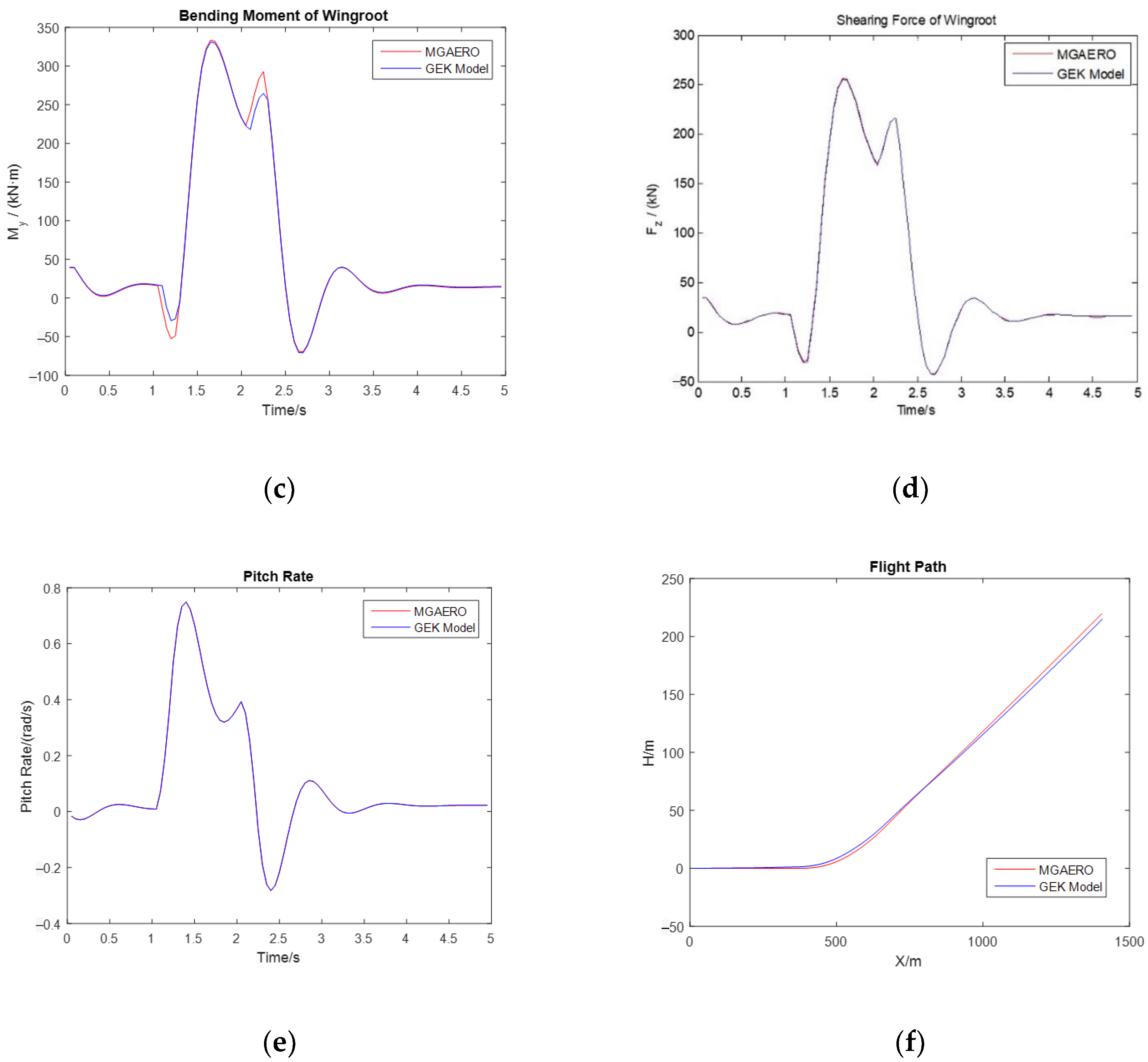
Then, the nonlinear flight load analysis is performed.

Table 8. Control surface deflection (based on nonlinear aerodynamics).

Model	Initial Angle of Attack (°)	Initial Aileron Angle (°)	Max Aileron Angle (°)
MGAERO	1.6764	−1.7685	−8.8808
GEK Model	1.6764	−1.7685	−8.8808

details the initial control surface deflection used during the maneuvering process, while Figure 11 illustrates the variations in the N factor, angle of attack, pitching rate, bending moment, and shearing force of the wing root of the example aircraft during the maneuvering process over a random flight time. A comparison of peak values for various parameters in the load during the maneuver is shown in

Table 9. Comparison of peak value in flight load analysis during maneuvering process (based on nonlinear aerodynamics).

Model	N Factor	Angle of Attack (rad)	Pitching Rate (rad/s)	Bending Moment of Wing Root (kN·m)	Shearing Force of Wing Root (kN)	Flight Altitude (m)
MGAERO	9.001	0.1546	0.5944	298.9	227.1	219.5
GEK Model	9.001	0.1546	0.5944	297.5	226.0	214.9

.

3.3. Accuracy of the GEK Model

In this section, an error analysis is conducted from two perspectives—numerical error and curve fitting—to assess the accuracy of the GEK surrogate model.

For m samples $\left(x_1,y_1\right),\left(x_2,y_2\right),\dots ,\left(x_m,y_m\right)$, with the predicted values from a certain model $\left(x_1,{\stackrel{⌢}{y}}_1\right),\left(x_2,{\stackrel{⌢}{y}}_2\right),\dots ,\left(x_m,{\stackrel{⌢}{y}}_m\right)$, we calculate the total sum of squares TSS for the samples:

$$TSS={\displaystyle \sum _{i=1}^m{\left(y_i-\overline{y}\right)}^2}$$

(21)

Next, we calculate the residual sum of squares RSS:

$$RSS={\displaystyle \sum _{i=1}^m{\left({\stackrel{⌢}{y}}_i-y_i\right)}^2}$$

(22)

We define $R^2=1-RSS/TSS$, that is,

$$R^2=1-\frac{{\displaystyle \sum _{i=1}^m{\left({\stackrel{⌢}{y}}_i-y_i\right)}^2}}{{\displaystyle \sum _{i=1}^m{\left(y_i-\overline{y}\right)}^2}}$$

(23)

The larger the value of $R^2$, the better the fitting effect. Taking $R^2$ as the curve fitting degree, we conduct an overall analysis of the variation curve of flight maneuvering loads during the maneuver.

In the steady-state pitching condition trim calculation, the GEK model predicts a very high aileron deflection angle.

In the abrupt pitching condition trim calculation,

Table 10. Fitting degree of flight load prediction curves during a maneuver.

	N Factor	Angle of Attack	Pitching Rate	Bending Moment of Wing Root	Shearing Force of Wing Root	Flight Path
GEK model (based on linear aerodynamics)	0.9999	0.9997	0.9999	0.9979	0.9977	0.9999
GEK model (based on nonlinear aerodynamics)	0.9999	0.9999	0.9999	0.9999	0.9999	0.9999

provides the fitting degree of the predicted flight loads during the maneuver. The prediction errors for longitudinal N factor, angle of attack, and pitching rate over time are small. In the curves of the bending moment and shearing force of wing root over time, only a few points have relatively large errors, typically near the turning points of the curves. Overall, the curve goodness of fit is above 95%.

Table 11. Peak error of GEK model in flight load prediction during maneuvering process.

	N Factor	Angle of Attack	Pitching Rate	Bending Moment of Wing Root	Shearing Force of Wing Root	Flight Path
GEK model (based on linear aerodynamics)	0.001%	0.008%	0.001%	0.28%	0.40%	0.57%
GEK model (based on nonlinear aerodynamics)	0	0	0	0.0047%	0.0048%	0.12%

compares the peak values of various parameters during the maneuvering process. The relative errors are all below 1%, and the absolute errors are minimal compared to the magnitude of the flight loads.

In the flight load analysis of the maneuver, under the requirement of recovering to level flight after achieving the same 9g longitudinal load, the predictive accuracy of the GEK surrogate model based on both linear and nonlinear aerodynamics is very high.

From the results, we obtain the following:

• Both the GEK surrogate models based on linear and nonlinear aerodynamics have a high prediction accuracy, enabling accurate trim calculations and predictions of flight load variation curves during maneuvers.
• Directly solving aerodynamic/structural coupling results in a time expenditure on the order of 100 s for a single load calculation, whereas using the GEK surrogate model for a single load calculation requires less than 1 s, showing a significantly improved computational efficiency.
• The trim calculation results based on nonlinear aerodynamics are superior to those with linear aerodynamics, and the difference between the two is significant. This indicates that conducting analyses based on nonlinear aerodynamics is necessary, especially in flight conditions with strong aerodynamic nonlinearity.

4. Conclusions

This study proposes an efficient flight load analysis method based on the GEK surrogate model. To validate the method, we use a numerical example to predict flight loads during longitudinal maneuvers of a flying-wing aircraft. The following conclusions can be drawn:

• The proposed method exhibits a good fitting accuracy that meets the requirements of flight load analysis and improves computational efficiency significantly.
• The variation in loads corresponds to the maneuvering flight processes. Because of the differences in aerodynamic force distribution, nonlinear aerodynamic forces and their surrogate models represent significant disparities or even inconsistencies in the variation trends of flight loads compared with linear aerodynamic forces. Hence, employing nonlinear aerodynamics for maneuvering flight process calculations is more rational.
• The GEK surrogate model relies on selecting sample databases and the accuracy of gradient calculations during model training. Compared to the Kriging surrogate model, the GEK model is more time-consuming and requires greater computational resources for model training and testing. However, it exhibits a higher fitting accuracy in strongly nonlinear scenarios.
• In future work, more complex maneuvers, such as rolling and other lateral maneuvers, will be analyzed. The existing elastic correction methods of aerodynamic forces will be improved, such as using the more accurate third-order surface panel method.

References

- Wang, Q.; Cai, J.S. Unsteady aerodynamic modeling and identification of airplane at high angles of attack. Acta Aeronaut. Astronaut. Sin. 1996, 17, 391–398. (In Chinese) [Google Scholar]
- Lin, G.-F.; Lan, C.; Brandon, J. A generalized dynamic aerodynamic coefficient model for flight dynamics applications. In Proceedings of the 22nd Atmospheric Flight Mechanics Conference, New Orleans, LA, USA, 11–13 August 1997. [Google Scholar]
- Goman, M.; Khrabrov, A. State-space representation of aerodynamic characteristics of an aircraft at high angles of attack. In Proceedings of the Astrodynamics Conference, Hilton Head Island, SC, USA, 10–12 August 1992; pp. 759–766. [Google Scholar]
- Wang, C.; Wang, G.D.; Bai, P. Machine learning method for aerodynamic modeling based on flight simulation data. Acta Aerodyn. Sin. 2019, 37, 488–497. (In Chinese) [Google Scholar]
- Zhang, W.; Wang, B.; Ye, Z.; Quan, J. Efficient Method for Limit Cycle Flutter Analysis Based on Nonlinear Aerodynamic Reduced-Order Models. AIAA J. 2012, 50, 1019–1028. [Google Scholar] [CrossRef]
- Kou, J.; Zhang, W. Reduced-order modeling for nonlinear aeroelasticity with varying Mach numbers. J. Aerosp. Eng. 2018, 31, 04018105. [Google Scholar] [CrossRef]
- Kou, J.; Zhang, W. Multi-kernel neural networks for nonlinear unsteady aerodynamic reduced-order modeling. Aerosp. Sci. Technol. 2017, 67, 309–326. [Google Scholar] [CrossRef]
- Han, Z.H. Kriging surrogate model and its application to design optimization: A review of recent progress. Acta Aeronaut. Astronaut. Sin. 2016, 37, 3197–3225. (In Chinese) [Google Scholar]
- Liu, Y.Z.; Wan, Z.Q.; Li, Q.; Zhang, Q.H. A Corrected Nearest Neighbor Transpotation Method of Aerodynamic Force for Fluid-Structure Interactions. Int. J. Numer. Anal. Model. 2020, 17, 746–765. [Google Scholar]
- Krige, D.G. A statistical approach to some basic mine valuation problems on the Witwatersrand. J. South. Afr. Inst. Min. Metall. 1951, 52, 119–139. [Google Scholar] [PubMed]
- Matheron, G. Principles of geostatistics. Econ. Geol. 1963, 58, 1246–1266. [Google Scholar] [CrossRef]
- Sacks, J.; Welch, W.J.; Mitchell, T.J.; Wynn, H.P. Design and Analysis of Computer Experiments. Stat. Sci. 1989, 4, 409–423, 415. [Google Scholar] [CrossRef]
- Liu, J.; Han, Z.-H.; Song, W.-P. Efficient kriging-based aerodynamic design of transonic airfoils: Some key issues. In Proceedings of the 50th AIAA Aerospace Sciences Meeting Including the New Horizons Forum and Aerospace Exposition, Nashville, TN, USA, 9–12 January 2012. [Google Scholar]
- Han, Z.H.; Zhang, K.S.; Song, W.P.; Liu, J. Surrogate-based aerodynamic shape optimization with application to wind turbine airfoils. In Proceedings of the 51st AIAA Aerospace Sciences Meeting Including the New Horizons Forum and Aerospace Exposition, Grapevine, TX, USA, 7–10 January 2013; p. 1108. [Google Scholar]
- Wang, X.F.; Xi, G. Aerodynamic optimization design for airfoil based on kriging model. Acta Aeronaut. Astronaut. Sin. 2005, 25, 545–549. (in Chinese). [Google Scholar]
- Zhang, K.S.; Han, Z.H.; Li, W.J.; Li, X. Multidisciplinary aerodynamic/structural design optimization for high subsonic transport wing using approximation technique. Acta Aeronaut. Astronaut. Sin. 2006, 27, 810–815. (In Chinese) [Google Scholar]
- Allen, M.J.; Dibley, R.P. Modeling Aircraft Wing Loads from Flight Data Using Neural Networks; NASA Dryden Flight Research Center: Edwards, CA, USA, 2003. [Google Scholar]
- Haas, D.J.; Milano, J.; Flitter, L. Prediction of Helicopter Component Loads Using Neural Networks. J. Am. Helicopter Soc. 1995, 40, 72–82. [Google Scholar] [CrossRef]
- Wallach, R.; de Mattos, B.S.; da Mota Girardi, R. Aerodynamic coefficient prediction of a general transport aircraft using neural network. In Proceedings of the 25th Congress of the International Council of the Aeronautical Sciences 2006, Hamburg, Germany, 3–8 September 2006; pp. 1199–1214. [Google Scholar]
- He, F.; Shu, C. Application of BP neural networks based on Bayesian regularization to aircraft wing loads analysis. Flight Dyn. 2009, 27, 85–88. [Google Scholar]
- Li, H.; Chen, X.; Zuo, L.; Zhao, Z. Surrogate model for flight load analysis based on random forest. Acta Aeronaut. ET Astronaut. Sin. 2022, 43, 309–318. (In Chinese) [Google Scholar]
- Jameson, A. Optimum aerodynamic design using CFD and control theory. In Proceedings of the 12th Computational Fluid Dynamics Conference, San Diego, CA, USA, 19–22 June 1995; pp. 926–949. [Google Scholar]
- Chung, H.-S.; Alonso, J.J. Using gradients to construct cokriging approximation models for high-dimensional design optimization problems. In Proceedings of the 40th AIAA Aerospace Sciences Meeting and Exhibit 2002, Reno, NV, USA, 14–17 January 2002. [Google Scholar]
- Chung, H.-S.; Alonsoy, J.J. Design of a low-boom supersonic business jet using cokriging approximation models. In Proceedings of the 9th AIAA/ISSMO Symposium on Multidisciplinary Analysis and Optimization 2002, Atlanta, GA, USA, 4–6 September 2002. [Google Scholar]
- Liu, W.; Batill, S.M. Gradient-enhanced response surface approximations using kriging models. In Proceedings of the 9th AIAA/ISSMO Symposium on Multidisciplinary Analysis and Optimization 2002, Atlanta, GA, USA, 4–6 September 2002. [Google Scholar]
- Laurenceau, J.; Sagaut, P. Building Efficient Response Surfaces of Aerodynamic Functions with Kriging and Cokriging. AIAA J. 2008, 46, 498–507. [Google Scholar] [CrossRef]
- Lu, W.; Wang, S.; Ma, Y. Static aeroelastic optimization of a high-aspect-ratio composite wing based on CFD/CSD and Kriging model. Chin. J. Appl. Mech. 2015, 32, 581–585+703–704. (In Chinese) [Google Scholar]
- Chen, L.; Qiu, H.; Gao, L.; Jiang, C.; Yang, Z. Optimization of expensive black-box problems via Gradient-enhanced Kriging. Comput. Methods Appl. Mech. Eng. 2020, 362, 112861. [Google Scholar] [CrossRef]
- MSC.Software. MSC Nastran 2001 Release Guide; MSC Software Corporation: Newport Beach, CA, USA, 2002. [Google Scholar]
- Liu, Y.; Wan, Z.; Yang, C. Quadratic programming equivalent mapping method for external aerodynamic force in flight load analysis. Beijing Hangkong Hangtian Daxue Xuebao/J. Beijing Univ. Aeronaut. Astronaut. 2020, 46, 541–547. (In Chinese) [Google Scholar]
- Butcher, J.C. A history of Runge-Kutta methods. Appl. Numer. Math. 1996, 20, 247–260. [Google Scholar] [CrossRef]
- Lophaven, S.N.; Nielsen, H.B.; Sondergaard, J.; Dace, A. A Matlab Kriging Toolbox; Technical University of Denmark, Informatics Math and Modelling TR 2002-12: Kongens Lyngby, Denmark, 2002. [Google Scholar]
- Dong, G.; Wang, X.; Liu, D. Metaheuristic Approaches to Solve a Complex Aircraft Performance Optimization Problem. Appl. Sci. 2019, 9, 2979. [Google Scholar] [CrossRef]
- Liu, W. Development of Gradient-Enhanced Kriging Approximations for Multidisciplinary Design Optimization; University of Notre Dame: Notre Dame, IN, USA, 2003. [Google Scholar]
- Laurenceau, J.; Meaux, M.; Montagnac, M.; Sagaut, P. Comparison of Gradient-Based and Gradient-Enhanced Response-Surface-Based Optimizers. AIAA J. 2010, 48, 981–994. [Google Scholar] [CrossRef]
Figure 1.
Coordinate axis and force analysis of symmetric maneuvering loads.
Figure 2.
Analysis of maneuvering loads.
Figure 3.
Prediction of nonlinear function using Kriging and GEK (20 samples).
Figure 4.
Prediction of nonlinear function using Kriging and GEK (40 samples).
Figure 5.
Analysis flowchart of maneuvering flight loads based on surrogate aerodynamic model.
Figure 6.
Illustration of the flying-wing aircraft.
Figure 7.
Structural finite element model and aerodynamic mesh grids of MSC.NASTRAN. (a) Structural finite element model. (b) Aerodynamic mesh grid.
Figure 8.
Aerodynamic mesh grids of MGAERO.
Figure 9.
Trapezoidal control input waveform.
Figure 10.
Variation curves of flight loads during a random dynamic process (based on linear aerodynamics). (a) N factor. (b) Angle of attack. (c) Bending moment of wing root. (d) Shearing force of wing root. (e) Pitching rate. (f) Flight path.
Figure 11.
Variation curves of flight loads during a random dynamic process (based on nonlinear aerodynamics). (a) N Factor. (b) Angle of attack. (c) Bending moment of wing root. (d) Shearing force of wing root. (e) Pitching rate. (f) Flight path.