Free and Forced Vibration of Laminated and Sandwich Plates by Zig-Zag Theories Differently Accounting for Transverse Shear and Normal Deformability


Dipartimento di Ingegneria Meccanica e Aerospaziale, Politecnico di Torino, Corso Duca degli Abruzzi 24, 10129 Torino, Italy
*
Author to whom correspondence should be addressed.
†
These authors contributed equally to this work.
Aerospace 2018, 5(4), 108; https://doi.org/10.3390/aerospace5040108
Submission received: 13 September 2018
/
Revised: 4 October 2018
/
Accepted: 8 October 2018
/
Published: 11 October 2018
(This article belongs to the Special Issue Adaptive/Smart Structures and Multifunctional Materials in Aerospace)
Abstract
:A number of mixed and displacement-based zig-zag theories are derived from the zig-zag adaptive theory (ZZA). As a consequence of their different assumptions on displacement, strain, and stress fields, and layerwise functions, these theories account for the transverse shear and normal deformability in different ways, but their unknowns are independent of the number of layers. Some have features that are reminiscent of ones that have been published in the literature for the sake of comparison. Benchmarks with different length-to-thickness ratios, lay-ups, material properties, and simply supported or clamped edges are studied with the intended aim of contributing toward better understanding the influence of transverse anisotropy on free vibration and the response of blast-loaded, multilayered, and sandwich plates, as well as enhancing the existing database. The results show that only theories whose layerwise contributions identically satisfy interfacial stress constrains and whose displacement fields are redefined for each layer provide results that are in agreement with elasticity solutions and three-dimensional (3D) finite element analysis (FEA) (mixed solid elements with displacements and out-of-plane stresses as nodal degrees of freedom (d.o.f.)) with a low expansion order of polynomials in the in-plane and out-of-plane directions. The choice of their layerwise functions is shown to be immaterial, while theories with fixed kinematics are shown to be strongly case-sensitive and often inadequate (even for slender components).

1. Introduction
Fibre-reinforced laminated and sandwich composites are fundamental to obtain a faster speed, longer range, larger payloads, less engine power, and a better operating economy of land, sea, and aerospace vehicles. Indeed, they possess excellent specific strength and stiffness properties along with many other advantages. However, their behaviour may be strongly influenced by local effects in their multi-phase structure, which can cause a relevant loss of strength and stiffness, and even lead to a possible catastrophic failure in service. To avert this, a three-dimensional description of their displacement and stress fields is required in the computer simulations. Displacements are no longer C1-continuous as in homogeneous non-layered materials, but instead they should be C0-continuous (zig-zag effect), this being the only way to guarantee the continuity of transverse shear and normal stresses and of the transverse normal stress gradient that is necessary to satisfy the fulfillment of local equilibrium equations in layered materials.
A multitude of theories is currently available for laminated and sandwich composites, which account for layerwise effects at varying degrees of accuracy and computational costs. The papers by Carrera et al. [1,2] and by Demasi [3] are cited wherein a broad discussion of this matter can be found. Theories can be summarily categorized into equivalent single-layer (ESL), discrete-layer (DL), and zig-zag (ZZ) formulations, and further into displacement-based and mixed theories, because displacements, strains, and stress fields can be chosen separately from one another.
Given the limited accuracy offered by ESL even to predict overall response quantities for certain loading, material properties, and stack-up [4,5], they still remain widespread by virtue of their low computational cost (see Burlayenko et al. [6] and by Jun et al. [7]), but nowadays, DL and ZZ are becoming more and more widespread in their applications. Indeed, they have the merit of accurately predicting the displacement and stress fields irrespective of lay-up, layer properties, and loading or boundary conditions. However, DL could overwhelm the computational capacity when structures of industrial interest are analysed (unless their use is limited to critical areas) due to having too many variables. Instead, ZZ having intermediate characteristics between ESL and DL can strike the right balance between accuracy and cost-saving, allowing designers’ demand of theories to be met in a simple, already accurate form. In particular, ZZ accounting for the transverse normal deformability effect has been proven to be suitable for carrying out ply-level stress analyses at a lower cost than DL.
Relevant examples of dynamic studies carried out by DL and ZZ that highlight their superior performance include the papers by [1,2,3,6,7] Boscolo and Banerjee [8], Khdeir and Aldraihem [9], Sayyad and Ghugal [10], Kazanci [11], Lin and Zhang [12], Vescovini et al. [13], and in addition to the previous ones, [14,15,16,17,18,19] are also cited. Moreover, papers [1,2,3,4,5,8,13,20] are examples that prove the limitations of ESL and the importance of the transverse normal deformability under static localised loading for certain boundary conditions and lay-ups [21] and even for accurately predicting the first free-vibration mode frequencies. Although ZZ theories are ultimately finding an ever-increasing number of applications thanks to their accuracy at an affordable cost, the literature shows that undeservedly Di Sciuva’s zig-zag-like fuction DZZ is less used than Murakami’s zig-zag-like fuction MZZ (for a definition of acronyms, see Table 1), despite their better accuracy with a low order of expansion of analytical solutions, as also demonstrated by the numerical results of this paper.
To contribute to the dissemination of DZZs and their further development, hereafter the typologies and specific characteristics of available ZZs are briefly reviewed. The intended aim is to explain the different behaviour of DZZ and MZZ as a consequence of their different layerwise contributions, namely Di Sciuva’s [22] (DZZ) or Murakami’s [23] (MZZ) zig-zag functions.
DZZ incorporates layerwise contributions as the product of assumed zig-zag functions and zig-zag amplitudes, the latter being computed to a priori satisfy the interfacial compatibility of out-of-plane stresses (for this reason, they are referred in literature as physically-based ZZ). Instead, MZZ assumes zig-zag functions that a priori feature a periodic change of the slope of displacements at interfaces, irrespective of the stack-up. As a consequence, stresses are assumed apart from the kinematics within the framework of Hellinger–Reissner variational theorem. For this reason, they are called kinematic-based ZZ. So, the development of MZZ is easier, and an efficient C0 formulation can more easily be generated, but they could not appropriately represent the displacement fields when the orientation angle of layers is aperiodic, as shown in the literature. According to findings by [1,2,5,24,25,26], it can be stated in general that MZZ are accurate only with a rather high expansion order of variables across the thickness and in the in-plane directions. As shown in [27,28,29,30,31,32,33], instead, DZZ accurately predict displacements and (very often but not in all cases) stresses with a lower expansion order.
As shown in the papers by Carrera et al. [1,2,24,25,26], Demasi [3], Mattei and Bardella [27], Icardi et al. [28,29], Li and Liu [30], Zhen and Wanji [31,32], and Shariyat [33], the transverse normal deformability, which is usually neglected because it is erroneously considered of little importance, on the contrary should be accounted for. Indeed, his contribution becomes of primary importance when boundary conditions other than simply-supported edges are considered, under a strong variation of mechanical properties across the thickness and for localised loading. However, a rather complex formulation of theories, i.e., with a sufficient number of parameters that can be defined in order to satisfy all of the relevant physical constraints, is required for these cases. Although very often power and Taylor’s series expansions are used across the thickness, hierarchic polynomials, and trigonometric and exponential functions, a combination of both or radial basis functions could be required to more efficiently represent variables [34,35,36,37,38,39].
The idea of separately hiring kinematics and stresses, so as to account for the transverse normal deformation without having to represent in a piecewise way the transverse displacement, was applied by Barut et al. to DZZ [40]. Other mixed DZZ that are based on a similar idea have a rather simple kinematics, but yet, the capability to quite accurately predict stresses has been formerly developed in HR form by Kim and Cho [41] and Tessler et al. [42]
Despite the notable contributions mentioned up to now, further research is required on ZZ because recent studies by Zhen and Wanji [43], Gherlone [44], and Groh and Weaver [45] have shown that MZZ could be less accurate than RZT [42], assuming the same degree of representation across the thickness, while [43] shows just the opposite for different cases. So, it is necessary to ascertain even whether three-dimensional (3D) DZZ can be as accurate as MZZ with a minor computational burden, so as to be effectively suitable for industrial purposes, considering also other theories in addition to those already examined in [44,45], especially those with a piecewise representation of the transverse displacement.
A massive amount of free vibration studies is currently found in the literature for cross-ply laminates, but other boundary conditions and lay-up that are equally interesting for practical applications need to be considered when testing the accuracy of theories (see, e.g., Li et al. [46]). It should be noted that for clamped edges, an incorrect vanishing transverse shear force resultant is predicted by ESL plate models; therefore, it is necessary to check on an adequate number of cases as to whether DZZ are immune from such mistakes. Also, lay-ups with a quite large variation of properties of layers, and in particular soft-core sandwiches, should be investigated to enhance the existing database. Another subject that needs further studies is what happens when zig-zag functions that are different from those commonly used [22,23] are assumed. It is also necessary to better clarify what effects have an a priori assumption of certain zig-zag amplitudes at certain interfaces, or even to all of the interfaces such as in MZZ, in order to save costs.
To contribute to this matter, in this paper, zig-zag theories in displacement-based and mixed form are particularized from the ZZA 3D zig-zag theory [29], assuming different layerwise functions. Consider that ZZA, here schematically defined as the adaptive zig-zag theory, assumes a variable kinematics with fixed degrees of freedom (d.o.f.) that consist of in-plane and transverse displacements , and transverse shear rotations at a middle reference plane. Moreover, it should be noticed that ZZA is capable of great accuracy, even with strong anisotropy at a cost that is still comparable to that of ESL.
The purpose of this paper is to test the accuracy of theories derived from ZZA under simplified hypotheses on displacement, deformations, and stress fields, so as to further reduce the computational cost, in order to assess whether and when the accuracy of ZZA can be preserved. The accuracy and the efficiency of these theories, which for the most part allow a redefinition of the coefficients layer-by-layer so as to satisfy all of the physical constraints and account for the normal transverse deformability effect (although in different ways), are assessed considering the free vibration and the response behaviour of blast-loaded multilayered and sandwich plates.
A new theory referred to as ZZA* is developed from ZZA in order to prove that once the coefficients of displacements are redefined across the thickness, the same accuracy degree can be achieved irrespective of the layerwise functions that are chosen. It will also be shown that as the coefficient is redefined, the same results are obtained even when zig-zag contributions do not explicitly appear. Other theories have been previously developed by the authors [47] in displacement-based and mixed form, either with Di Sciuva’s or Murakami’s zig-zag-like functions, and which also have characteristics similar to other theories that are already known in the literature, are considered for comparison.
Numerical applications aim to show the superiority of ZZA* over ZZA, including its lower computational costs with the same accuracy, for the quite large range of variation of lay-ups and boundary conditions that are considered. Benchmarks that are either retaken from the literature or new are considered, the former in order to enable a comparison of available theories, and the latter in order to enhance the existing database. The results by the present theories are compared to exact solutions whenever available or to 3D finite element analysis (FEA) [48]. The findings can be categorized as the new results of known benchmarks provided by the new theories and entirely new results for the new benchmarks, which could serve as test beds for future analytical and finite element models.
This study also aims to show the superiority of ZZA* over all of the other theories considered for most of the cases, since the use of simplified assumptions implies a loss of accuracy. It will be shown that the accuracy of the simplified theories, in particular those of Murakami, is strongly case-sensitive; therefore, they cannot be used interchangeably. Studies are carried out in closed form considering the free and forced vibrations of laminated and sandwich beams and plates, simply-supported and clamped edges, different lay-ups, and distinctly different material properties of constituent layers, so as to give rise to relevant 3D effects.
2. Preliminaries and Notations
Constituent layers are assumed to have a uniform arbitrary thickness and linear elastic properties. They are assumed to be perfectly bonded to each other and, as usual when the global-scale response is examined, the existing bonding resin interlayer is disregarded. For the same reason, sandwiches are described in homogenised form as multilayered structures with one or more thick soft intermediate layers as the cores, with the cell-scale effects being disregarded.
A rectangular, right-handed Cartesian coordinate reference system () is assumed as the reference frame, having () on the middle reference plane of the laminated plate (origin in the lower left edge) and as the thickness coordinate (, with being the overall thickness). Lx and Ly symbolise the plate side-length in the x and y-directions, while and represent the upper and lower positions of the layer interfaces, respectively. Subscripts k and superscripts k are used to indicate that a quantity belongs to the layer , while u and l mark the upper and lower faces of the laminate, and a comma is used to indicate spatial derivatives, e.g., , . The elastic in-plane and transverse displacement components are indicated as and , respectively. Strains are assumed to be infinitesimal and, to distinguish their origin, they are specified as , , respectively when they come from kinematic or stress-strain relations. Once assumed as primary variables, they are indicated as , , (; , ; ; ). Stresses from stress–strain constitutive relations are indicated as , while when they are assumed as primary variables, they are indicated as , , .
2.1. Recalls on Mixed Variational Theorems
Here a generalized version of Hu-Washizu theorem is used, whose primary displacement boundary condition link is weakened as and which generates the following variational statement:
Here represents the canonical functional, are the components of the external unit normal to the volume bounding surface, are the components of body forces (they will contain inertial forces, as explained in (4)) and , ensure the consistency of assumed strain and stress fields with their counterparts obtained from stress-strain and strain-displacement relations. As usual, the prismatic volume of the laminated plates is assumed to be bounded by a surface that is split into a surface on which surface tractions are prescribed and a surface on which surface displacements are prescribed. Body forces on , prescribed surface tractions on and prescribed displacements on are assumed to act.
Theories with displacements and out of plane stresses assumed separately are developed from the HR variational theorem:
where is the first variation of the HR canonical functional, and the following assumptions are made: ; , being ; .
Dynamic governing equations are obtained from the previous variational statements (1), (2), or from the principle of virtual work (PVW), for theories in displacement-based form, accounting for the work of inertial forces.
2.2. Construction of Analytical Solutions
Closed-form solutions to dynamic governing equations are obtained, irrespective of the theory examined, expressing functional d.o.f. as a truncated series expansion of unknown amplitudes and trial functions that individually satisfy the prescribed boundary conditions:
Then, we substitute these expressions within PVW, HR, or HW functionals and operating as specified immediately below. Here, symbolises in turns , , , , , because middle plane displacements and rotations of the normal are assumed as the only functional d.o.f. for each theory of this paper. Mechanical boundary conditions are accounted for by determining a number of unknown amplitudes , in proportion to the number of boundary conditions enforced, using the Lagrange multipliers method to account for the relationships resulting from each mechanical condition. The remaining amplitudes are determined deriving the governing functional with respect to still unknown amplitudes and equating to zero, having considered the work of inertial forces:
within the functionals. In this way, an algebraic system is obtained whose solution provides the numerical value of each amplitude; then, the displacement, strain, and stress fields can be computed.
Since symbolic calculus being used to construct the theories, the applied distributed loading can be conveniently defined as a continuous or discontinuous general function acting on upper and/or lower faces (or just on a part of them), so that energy contributions can be constructed in exact closed form. In this way, a series expansion representation with a large number of components is not necessary to represent discontinuous or otherwise complex loading distributions; then, the construction of the structural model in the numerical applications can be simplified, and at the same time made more accurate.
The trial functions have been adopted in individual applications are explicitly defined below and in Table 2 along with the expansion order used in each case. Note that although it is different for each benchmark, the order of expansion used is the same for all theories when a specific one is examined being equal to the minimum one that makes ZZA accurate. This is done to homogenise results and in order to compare theories under the same conditions.
At the clamped edge of cantilever beams, hereafter assumed at by way of example, the following conditions are enforced
the following further conditions are enforced:
to simulate that (5) holds identically across the thickness. To ensure that the transverse shear stress resultant force equals the constraint force, the following additional constraint
is enforced, while at the free edge x = L such resultant force is enforced to vanish
It should be noted that the boundary conditions in Equations (6) to (8) are enforced using Lagrange multipliers methods; no further conditions are enforced on bending moments, but if necessary, they could be coerced choosing the sufficient expansion order in Equation (3).
At the supported edge of the propped cantilever beams at x = L, the following support condition:
is enforced at the lower face , while the condition in Equation (8) is reformulated as:
At the simply supported edges, the following boundary conditions are enforced
on the reference mid-plane of plates at , , and , . Appropriate changes corresponding to the ones for simply supported beams are obtained. Table 2 provides the trial functions and expansion order that is assumed for each benchmark.
Any other boundary condition could be enforced in the same way, namely by choosing the trial functions that individually satisfy the prescribed boundary conditions. In the event of this not being possible and in order to satisfy the mechanical conditions, Lagrange multipliers method should be applied. In the numerical applications for cases g and h, the boundary condition to be further enforced is , because some of their first free vibration modes exhibit anti-symmetric displacements in the transverse direction. In this way, a closed-form solution can be obtained with a reduced computational effort, instead of resorting to FEA, as is often done for such cases.
3. Higher-Order Theories
The laminated plate theories that are used as structural models are thoroughly examined below. Here, they are grouped into higher-order and lower-order ones. The latter represent simplified versions of the former, having mostly features that are similar to those of the theories that have been previously proposed in the literature. In the following section, it will be specified which are new and which have been previously developed by the authors. Governing equations will not be reported in explicit form, as they can be obtained in a straightforward way using standard techniques.
3.1. Features of the ZZA Theory and the Higher Order Theories Derived from It
As it forms the basis of all theories considered in this paper, the theoretical framework of ZZA below is expounded first. The through-thickness displacement field is postulated as [29]:
Three kinds of contributions that are distinctly separated into lower-, higher- and layerwise are incorporated, whose specific purpose is described below.
- is a linear contribution and contains the five functional degrees of freedom of the theory.
- contains higher-order terms. Any combination of independent functions could be assumed to represent and ; however to include theory [28] as a particularization of ZZA [29], the following form is chosen:Higher-order contributions are characteristic of ZZA, while the terms , are the same as in the previous theory [28]. The closed-form expressions of coefficients , , to are obtained using symbolic calculus from enforcing the fulfilment of stress boundary conditionsHere, represents the distributed transverse loading acting on the upper and lower faces. Of course, also, non-homogeneous conditions could be enforced without any additional difficulty. For clarity, contributions from Equations (14) and (15) are rearranged in the following way:The lower-order contributions under the square brackets in Equation (17) are determined by enforcing the fulfilment of the boundary conditions in Equation (16) and the local equilibrium equations:at selected points across the thickness. Higher-order contributions , , which enable a variable-kinematics representation across the thickness, are computed for each fictitious computational layer in which the laminate is subdivided by imposing the fulfilment of Equation (18). However, except otherwise stated, a third/fourth-order representation that embraces the whole laminate is used in the applications which is adequate to obtain accurate results. Indeed, as shown in [21], this choice is a valuable combination of accuracy and cost-saving also when extreme variations of material properties give rise to very strong layerwise effects. A single computational layer is used for laminates, while two or three layers are used for sandwiches. Note that the in-plane position of equilibrium points can be chosen appropriately for each case.
- represents the layerwise contributions; the expressions of zig-zag amplitudes , and are determined so that the continuity of out-of-plane stresses and the transverse normal stress gradient at the layer interfaces is satisfied, as prescribed by the elasticity theory through the following stress compatibility conditions:at the physical and mathematical layer interfaces. Layerwise contributions and restore the continuity of displacements at the mathematical layer interfaces. The symbols and in the summation of Equations (12) and (13) are used to distinguish the number of physical interfaces from that of the mathematical layer interfaces, respectively. In detail, enables the continuity of transverse shear stresses, while , enable the continuity of the transverse normal stress and of its gradient at physical and mathematical layer interfaces. All together, these provide the right slope changes of displacements at the interfaces of layers with different material properties and/or orientations.
Elsewhere in this paper, the symbols − and + indicate the position just before and just after the interface, respectively. The term appearing in in Equations (12) and (13) is Di Sciuva’s zig-zag function [22], while is Icardi’s parabolic zig-zag function [28], with Hk being the Heaviside unit step function (Hk = 0 for z < zk, while Hk = 1 for z ≥ zk).
The enforcement of the equilibrium and stress compatibility conditions in Equations (18) and (19) yields to a system of algebraic equations at each interface that is solved in closed form once and for all using a symbolic calculus tool. Notice that if just the material properties and/or the orientation of layers change, but not their number, symbolic expressions representing the solution will remain the same.
It will be shown forward that and can be replaced with any other layerwise function keeping the results unchanged, provided that coefficients inside are re-computed for each computational layer, as outlined above. Layerwise functions can even be omitted if a sufficient number of coefficients are incorporated in whose expressions are determined by enforcing the fulfilment of the interfacial stress compatibility conditions in Equation (19). To show this, a new theory ZZA* is developed in Section 3.1.1, which is devoid of , but incorporates new unknown coefficients within , which will be indicated as . Since this choice speeds up the computations of the coefficients of each layer, it turns into a computational advantage that grows with the number of computational layers, so it is worth taking into consideration.
The expressions of and are determined in a straightforward way by enforcing the continuity of displacements at the mathematical layer interfaces
Notice that as no d.o.f. derivatives are involved, the computation of and is much easier and faster than those of , , and , which instead involve such derivatives. However, it must be considered that the computation of all of the above indicated zig-zag terms takes only an infinitesimal fraction of the overall calculation cost, and so remains compatible with that of ESL.
The strain energy updating technique (SEUPT) [29] can be used to obtain a C0 formulation of the ZZA theory, since derivatives of the d.o.f. are involved in the displacement field as a consequence of the enforcement of Equations (18) and (19).
3.1.1. ZZA* Displacement-Based Theory
This theory, which represents the new theoretical contribution brought by this paper, is developed with the intended aim to demonstrate that the choice of zig-zag functions is immaterial, provided that the coefficients of displacements are recomputed as indicated above.
For this purpose the displacement field of ZZA* is assumed to be similar to that of ZZA except for the layerwise functions. In numerical applications it will be shown that the same accuracy of ZZA can be achieved without explicitly incorporating contributions , and consequently obtaining a reduction of the computational burden.
It will be shown by the numerical results that the choice of zig-zag functions is immaterial if the coefficients are redefined layer-by-layer, so these functions do not even need to be explicitly incorporated in the displacement field. The same result wouldn’t be achieved by keeping the coefficients fixed across the thickness, in which case the accuracy depends on the choice of zig-zag functions.
The displacement field of ZZA* is conceived in the following way:
wherein the terms and serve the same purpose as and in Equation (12) inside ZZA, while and have the same function of and , and has the function of in Equation (13). In the same way of ZZA, , , , , and allow the stress boundary conditions in Equation (16) and the local equilibrium equations in Equation (18) to be met. More specifically, and enable the fulfillment of the stress boundary conditions concerning and over the lower bounding face, while they are cancelled in subsequent layers. Instead, , , , and allow satisfying the three equilibria (18) at two points for each intermediate layer. In the lower layer, such coefficients enable the two boundary conditions on to be enforced along with the three equilibrium equations at a single point. In this way, free variables still remain that allow meeting three equilibrium equations at a single point across the upper layer and the boundary conditions at the upper bounding surface. When more equilibrium points are desired, each layer can be subdivided into two or more computational layers. However, this doesn’t mean an increased expansion order or number of variables, since coefficients can be recomputed using the same order of representation for each computational layer, and the d.o.f. remain fixed. As for ZZA, closed-form expressions of all of the coefficients of ZZA* within contributions are determined once and for all for a specific lay-up using a symbolic calculus tool.
3.2. HWZZ Mixed Theory
Such a theory was developed in [47] in order to reduce the computational effort of ZZA by keeping only the essential contributions to the displacement, strain, and stress fields, and hopefully preserving its accuracy. Developed within the framework of the Hu–Washizu theorem, HWZZ forms the basis of another mixed theory here used and called HWZZM, which considers a different zig-zag layerwise function.
3.2.1. Master Displacements
The displacements of HWZZ are derived from those of ZZA neglecting the contributions of , because they are supposed to give imperceptible slope variations compared to those by , . Also higher-order and adaptive contributions and are neglected and no decomposition into mathematical layers is allowed. As a consequence, contributions by and are omitted. So, the displacement field of HWZZ is written:
3.2.2. Master Strains
Out-of-plane strains , , are constructed on the basis of the ZZA layer-by-layer representation of displacements as:
The symbol states that they refer to the computational layer . On the contrary, no decomposition into mathematical layers is allowed for the in-plane strains:
The expressions of membrane stresses , , and are obtained in a straightforward way from stress–strain relations and previous strains, while those of the out-of-plane counterparts are assumed as specified next.
3.2.3. Master Stresses
Out-of-plane stresses are obtained from membrane stresses by integrating local equilibrium equations:
and then
In this way, stress jumps resulting from the omission of contributions by are recovered. As a consequence of simplifying the assumptions that are made, HWZZ needs to be post-processed by ZZA in order to accurately represent displacements when very strong layerwise effects rise.
3.3. Other Mixed Theories
3.3.1. HWZZM Theory
Murakami’s zig-zag contributions are assumed [51], which are variations of the canonical form
where:
In fact, the displacement field of HWZZM is assumed as:
Differently to Murakami’s theories proposed in the literature, here, multiplier coefficients , , and are incorporated, which can be defined differently across the thickness to improve the accuracy. As has been done previously, their expressions are a priori determined by enforcing the continuity of the transverse shear and normal stress, and of the transverse normal stress gradient at layer interfaces, so that they are no longer uniform across the thickness. As before, and restore the continuity of displacements at interfaces of mathematical layers.
HWZZM is developed starting from the displacement field in Equations (29) and (30) in the same way as HWZZ; namely, the decomposition into fictitious computational layers is not allowed for the displacement and in-plane strain fields, while it is allowed for out-of-plane strains. Contributions to in-plane displacements over the third-order and to the transverse displacement over the fourth-order are neglected. Stress–boundary conditions are enforced at the top and bottom laminate faces, while local equilibrium equations are enforced at the inner layers. Membrane stresses , , and come from stress–strain relations, while out-of-plane master stresses are derived integrating local equilibrium equations. The numerical findings will show that although different zig-zag functions contradistinguish ZZA, HWZZ, and HWZZM, their results are indistinguishable, so there will be evidence that the choice of such functions is immaterial, provided that and are recomputed at each interface.
3.3.2. HWZZM* New Theory and Theories Derived from It
In order to assess the effect of the choice of different zig-zag functions, a new theory called HWZZM* is derived from ZZA*, similar to how HWZZ was derived from ZZA. Then, other theories are particularized from HWZZM, assuming , , and are equal to those at a specific interface, which differ from one another.
3.3.2.1. HWZZM* Theory
The displacement field of HWZZM* is assumed in the following form
whose amplitudes are computed at each interface from the enforcement of the stress compatibility conditions in Equation (19). In this case, terms only serve to satisfy the stress–boundary conditions and local equilibrium equations, while the satisfaction of stress compatibility conditions is demanded to .
It should be noted that Equations (31) and (32) imply a little reduction of the processing time, which is equal to 10% per each layer with respect to ZZA and to a somewhat lesser extent equal to 6% with respect to HWZZ. Of course, such an advantage will become more consistent as soon as the number of computational/constituent layers increase.
3.3.2.2. Theories with a Priori Chosen Zig-Zag Amplitudes
Several theories are particularized assuming a priori zig-zag amplitudes as the ones by HWZZM competing at a specific interface and then keeping them unchanged across the thickness, which is something similar to what is done using Murakami’s zig-zag functions, whose amplitudes are assumed a priori.
The amplitudes of HWZZMA are assumed to be coincident with those of HWZZM at the first interface from below, while the and of HWZZMB are assumed to be the same as those of HWZZMA at the first interface from below, but instead, is calculated as in HWZZM theory. In HWZZMC, only is assumed to be uniform across the thickness and coincident with that of HWZZM at the first interface from below, while the remaining are computed at each interface. are neglected in HWZZM0 theory, while and are assumed in the same way as HWZZMB.
The HWZZMB2 and HWZZMC2 theories are the same as those of HWZZMB and HWZZMC, respectively, but currently, the amplitudes are assumed to be coincident with those of HWZZM at the first interface from above. Since zig-zag amplitudes are assumed, discontinuous out-of-plane stress may result; hence, the integration of local equilibrium equations is required to obviate this discontinuity, with a corresponding increase in costs by 0.9%. However, it must be considered that zig-zag amplitudes are not being computed at each interface, so a processing time saving of 10% is obtained, and in the end, a positive balance is achieved. However, applications will show a loss of accuracy, making it vain.
4. Lower-Order Theories
Lower-order theories are particularized from ZZA through limiting assumptions that take features that are reminiscent to those of the theories in the literature.
4.1. MHR Theory
MHR considers piecewise cubic in-plane displacements, wherein Murakami’s zig-zag function in Equation (28) is incorporated as the layerwise function, alongside a fourth-order polynomial transverse displacement [47]:
Coefficients , , , , and are still calculated by enforcing the fulfilment of the stress boundaries conditions in Equation (16), while is calculated by enforcing the fulfilment of the first and second equilibrium in Equation (18) at the middle plane of the laminate. Since out-of-plane stresses may be still discontinuous at layer interfaces, and since is assumed to be uniform across the thickness, the expressions of out-of-plane stresses are derived integrating local equilibrium equations within the framework of an HR variational theorem (2). A refined version that is referred as MHR±, is obtained by determining the right sign of Murakami’s zig-zag function (28) on a physical basis, instead of being forced to reverse at interfaces by the coefficient . The right slope is determined at each interface without a cost burden evaluating what sign attain the lowest residual force norm from three local equilibrium equations.
4.2. MHR4, MHWZZA and MHWZZA4 Theories
A refined variant MHR4 of MHR is obtained assuming the in-plane displacement field by Equation (31), and a fourth-order piecewise variation of the transverse displacement [47]:
Coefficients to are determined by enforcing the fulfillment of the stress boundary conditions in Equation (16), whereas is calculated by enforcing the fulfilment of the third local equilibrium equation at the middle plane.
MHWZZA is developed assuming the same master displacement field as that of MHR in Equation (33) and the same master strain and stress fields as those of the HWZZ model, in Equations (25) and (26), respectively. To improve the accuracy, the displacement, strain, and stress fields of MHWZZA are recovered using ZZA as the post-processor.
Similarly to MHR±, a refined theory MHR4± is obtained from MHR4 determining the sign of Murakami’s zig-zag functions on a physical basis.
A further theory MHWZZA4 is derived assuming the in-plane displacement field in Equation (31) by MHR, the transverse displacement in Equation (13) by ZZA, and as the master strain and stress fields those by HWZZ in Equations (25) and (26), respectively. The only substantial difference of MHWZZA4 with respect to HWZZ and ZZA is a different zig-zag function; the just-mentioned theories along with ZZA* and HWZZM* make it possible to verify whether the accuracy is sensitive to the choice of zig-zag functions.
4.3. HRZZ and HRZZ4
HRZZ theory is developed postulating a uniform transverse displacement and a third-order zig-zag representation of in-plane displacements [47]:
Within the framework of the HR theorem, the transverse normal stress is assumed to be the same as that of the ZZA model, while the transverse shear stresses are derived from the equilibrium equations assuming kinematic relations in Equation (25) to define membrane stresses. However, currently, second and higher-order derivatives of the d.o.f. are neglected, and a unique computational layer is assumed. Since a uniform transverse displacement is chosen and transformed, reduced stiffness properties are assumed. Then, , is the inverse of ; ; ; ; , and .
In order to increase the accuracy of HRZZ, the ZZA theory will be used as the post-processor and the results obtained in this way will be indicated as HRZZ PP in the figures.
HRZZ4 assumes the same in-plane representation of HRZZ, the following fourth-order polynomial approximation of the transverse displacement [47]:
and the same stress fields of HRZZ. In this case, being no longer null, it is unnecessary to use transformed, reduced stiffness properties. Similar to in the previous theories, coefficients b to e of Equation (36) are determined by enforcing the stress boundary conditions at the upper and lower faces (16). The out-of-plane master shear stresses are obtained through integrating local equilibrium equations, while the appearing in Equation (2) is assumed to be the same as that of ZZA.
5. Numerical Assessments and Discussion
The accuracy of previous theories is assessed, analysing free vibration modes and the transient dynamic behaviour under impulsive loading of simply supported and clamped, laminated, and sandwich beams and plates.
The lay-up, geometric, and material properties of each case are grouped in Table 3 and Table 4; the trial functions and the expansion order that are used in each study are reported in Table 2; the normalization of quantities is brought in Table 5; while the results are carried in Table 6, Table 7, Table 8, Table 9, Table 10, Table 11, Table 12, Table 13, Table 14, Table 15, Table 16, Table 17, Table 18, Table 19 and Table 20 and the computational cost is reported in Table 21 and Table 22.
5.1. Propped Cantilever Sandwich Plate in Cylindrical Bending under Uniform Static Loading
Firstly, a static analysis of two propped cantilever sandwich plates in cylindrical bending under a uniform load on the top face are considered, in order to preliminary assess the accuracy of the theories in predicting the displacement and stress fields. The structure is clamped at x = 0 and restrained on the lower face at x = Lx; the elastic moduli of faces and core are assumed to be Eu/El = 1.6 and Eu/Ec = 166.6, respectively, and with a Poisson’s ratio ; the lower (l) and upper (u) faces are tl = c/2 and tu = c/4 thick, respectively, where c is the core thickness. The results of the theories are compared to the ones by 3D FEA [48], whose elements are formulated in order to fulfil Equations (16) and (18), and the displacements and out-of-plane stresses are assumed as nodal d.o.f. The length-to-thickness ratios Lx/h = 5.714 (case a1) and 20 (case a2) are considered.
Regarding case a1, according to Mattei and Bardella [27] and Icardi and Sola [21], its through-thickness displacement and stress fields are very challenging, and require a very accurate description of the transverse shear force resultant at the clamped (7) and at the simply supported edges (10), and a very accurate description of the transverse normal stress; otherwise, incorrect stress predictions are obtained. Moreover, what makes this a tough case is the opposite sign that is assumed at the upper and lower faces by the transverse shear stress at the supported edge. Figure 1 shows the results for the thickest case (Lx/h = 5.714). It can be seen that, contrary to what was postulated by Murakami’s zig-zag function, at the supported edge, the slope of never reverses, while doesn’t reverse near the upper interface, so MHR and MHR4 obtain inaccurate results. Even MHR± and MHR4±, whose interfacial displacement slope is determined on a physical basis, are not adequate, because their kinematics are too poor. MHWZZA4 and MHWZZA, incorporating strain and stress fields from HWZZ, obtain better results than MHR and MHR4, while HRZZ calculates an incorrect null transverse displacement at the supported edge. Summarizing, all of the lower-order theories obtain inaccurate results. Since the results of HWZZM are in good agreement with those of the adaptive theories ZZA, ZZA*, HWZZ, and 3D FEA, it is proven that the choice of layerwise functions is immaterial as long as higher-order coefficients are defined as in Section 3.1 and Section 3.3. HWZZMB, HWZZMB2, and HWZZM0 assuming arbitrarily zig-zag amplitudes can accurately predict the axial displacement but not the transverse one, while HWZZMC and HWZZMC2 calculate precise displacements, whereas HWZZMA always provides wrong results (so they are not reported in the figures). It should be noticed that the behaviour of theories arbitrarily assuming zig-zag amplitudes is very case-dependent, and only some are quite accurate.
The results for the slender case Lx/h = 20 are reported in Figure 2; the calculations show that a still significant difference between the predictions of theories exists, and differs from that which is expected for the rather thin sandwich structures. Again, only higher-order theories obtain a good degree of accuracy, and HWZZMA is so inaccurate that results cannot be reported. The obvious conclusion is that even for a length-to-thickness ratio of 20, an accurate description of kinematics is of primary importance in the present case.
On the basis of the processing time required (see Table 21 and Table 22 and Section 5.10), it can be concluded that the adaptive theories ZZA, ZZA*, HWZZ, HWZZM, and HWZZM* are the most efficient ones, as they combine accuracy and low cost. It should be remembered that the same representation with the same low expansion order (Section 2.2) dictated by industrial needs is used for all of the theories. Since the results in the literature for MZZ have shown that greatly increasing the expansion order along with that of the representation across the thickness obviously produces more accurate results, prior statements are valid only for the conditions that are examined here. Below, dynamic tests are carried out that consider progressively more challenging benchmarks that highlight the need for sophisticated theories.
5.2. Free Vibration Modes of Simply Supported Laminated and Sandwich Plates in Cylindrical Bending
First, the analysis of simply supported cross-ply [0/90/0] (case b1) and [0/90]2 (case b2) plates in cylindrical bending is presented, which primarily serves as a preliminary test of the accuracy of 3D FEA [48] in solving dynamics problems, this having yet been tested. Then, a [0/core/0] simply supported sandwich plate in cylindrical bending (cases b3) is studied, which has more marked layerwise effects.
The first fundamental frequency predicted by the present theories for case b1 is given in Table 6 considering a length-to-thickness ratio of 10. Comparisons are carried out with the exact solution and the results of EFSDT and EHSDT theories by Kim [49].
It can be seen that only ZZA, HWZZ, HWZZM, ZZA*, and HWZZM* higher-order theories provide very accurate results, but a sufficient accuracy is obtained by the HRZZ, HRZZ4, MHWZZA, MHWZZA4, MHR, MHR4, MHR±, MHR4±, and HWZZMC simplified theories. Instead, HWZZMA, HWZZMB, HWZZMB2, and HWZZM0 give an inaccurate prediction of it. However, case b1 does not appear to be severe, as many theories prove adequate. Although they have dissimilar characteristics, it is noted that HSDT and FSDT (shear correction factor of 5/6 chosen to minimize the error) calculate even the fundamental frequency inaccurately. The same considerations apply for case b2, with the same length-to-thickness ratio of 10, as shown in Table 6; therefore, the previous considerations are not repeated.
The fundamental frequency for a [0/core/0] simply supported sandwich plate constituting case b3 [49] is reported in Table 7 for three different length-to-thickness ratios (four, 10 and 20). Contrary to what one would expect, errors don’t dramatically decrease as Lx/h increases, and the behaviour of theories remains quite diversified. In particular, MHWZZA, MHWZZA4, and HWZZMA, HSDT, and FSDT (shear correction factor is 5/6) prove to be inaccurate irrespective of the length-to-thickness ratio.
Modal displacements and stresses are reported In Figure 3, Figure 4 and Figure 5, where the results are normalized as shown in Table 5, and show that the axial displacement and the in-plane stress are accurately calculated except by MHWZZA and MHWZZA4, while the transverse shear stress is inaccurately calculated by MHR, MHR4, MHR±, MHR4±, MHWZZA, and MHWZZA4 for the thickest case. An even bigger scattering is shown for , which is accurately calculated only by ZZA, HWZZ, HWZZM, ZZA*, and HWZZM*, while on the contrary, the transverse normal stress is accurately calculated by all of the theories. Note that the results by HWZZMA are never reported in Figure 3 and Figure 4 as being too wrong. For the same reason, the stress and displacement distributions are not reported for FSDT and HSDT. Such big errors highlight the inapplicability of the most simplified theories even for slender cases, which is contrary to what is often claimed in the literature.
5.3. Fundamental Frequency and Modal Displacements and Stresses of a Simply Supported, Anti-Symmetric Cross-Ply Plate
The fundamental frequency of [0/90/0/90], simply supported, cross-ply square plates with a length-to-thickness ratio of five [4], is examined in Table 8 for increasing the values of the degree of orthotropy E1/E2 ranging from three to 40 (case c1).
Comparisons are given with the results by a global–local higher-order theory [4] and by Matsunaga [56], which were obtained using a higher-order ESL. It can be seen that all of the theories of this paper provide fairly accurate predictions of the fundamental frequency in correspondence with the lowest orthotropy ratios, while quite dispersed results are shown as this ratio reaches the value of 20. In particular, very incorrect results are given by ESL, FSDT (shear correction factor ), and HSDT for E1/E2 values greater than 30 and by theories MHR, MHR4, MHWZZA, MHWZZA4, HWZZM0, HWZZMB2, and HWZZMC2. Adaptive theories ZZA, ZZA*, HWZZ, HWZZM, and HWZZM* instead always provide results that are in very well agreement with the exact solution, irrespective of the orthotropy ratio.
The through-thickness variation of modal displacement , transverse shear , and transverse normal modal stresses are reported in Figure 6 and Figure 7 for ratios E1/E2 of 3 and 40, respectively. Note that is correctly captured by all of the theories only for E1/E2 = 3, so just the results for this highest ratio are reported. The results by HWZZMB2 and by HWZZM0 are only reported for E1/E2 = 40, as they are inaccurate for all of the other cases. All of the other theories provide a quite accurate prediction of the in-plane displacement as well as of , with the only exceptions being MHR and MHR4, while there is a bigger scattering of results regarding .
The fundamental frequencies for case c2 with an orthotropy ratio E1/E2 of 30 and a length-to-thickness ratio of 10/3 are reported in Table 9. Modal displacements and modal in-plane and transverse shear and normal stresses for this case are shown in Figure 8, along with the results by 3D FEA, Zhen and Wanji [4], and Matsunaga [56]. These results show that MHWZZA, MHWZZA4, MHR, and MHR4 overestimate the fundamental frequency, while MHWZZA, MHWZZA4, MHR, and MHR4 incorrectly predict the in-plane displacement and stress, while MHR± and MHR4±, whose slope is defined on a physical basis, obtain better results than their counterparts MHR and MHR4 with the slope assumed a priori.
A rather large dispersion of results is shown for and for the transverse normal stress, while the transverse shear stress is erroneously provided by HRZZ, HRZZ4, MHWZZA, MHWZZA4, MHR, and MHR4 only across the first layer. Again, in this case, with the slope being defined on a physical basis, HSDT and FSDT (the latter uses π2/12 as the shear correction factor in order to improve the accuracy of the results) appear inadequate to perform the analysis.
5.4. Fundamental Frequency of a Cross-Ply Plate with Different Thickness Ratios and Boundary Conditions
The fundamental frequency of a [0/90/0] cross-ply square plate with a thickness ratio ranging from 4 to 100 and simply supported (case d1), all clamped, or simply supported edges and clamped on opposite sides (case d2), are reported in Table 10 and Table 11, respectively. The results are compared to those by Di Sciuva and Icardi [50] (RFSDT, RHSDT, theories and RHQ40 elements) and to 3D FEA [48], as well as to those by FSDT and HSDT.
The results of case d1 show a very well agreement among the theories each other, as well as with 3D FEA reference solutions when the length-to-thickness ratio increases, because the layerwise effects become less important, while remarkable differences are shown for the thickest cases. All of the theories appear to be accurate except for HWZZM0, MHWZZA, and MHWZZA4 (even for moderately thin plates), FSDT (shear correction factor 5/6), and HSDT (the latter two are accurate only for the lengths-to-thickness greater than 10).
The results for the different boundary conditions considered (case d2), namely clamped and simply supported edges (CSCS) and all-clamped edges (CCCC), are reported in Table 11 for a length-to-thickness ratio Lx/h = 10, along with the results for simply supported edges (SSSS).
It is noted that only ZZA, ZZA*, HWZZ, HWZZM and HWZZM* give predictions of the fundamental frequency that are always very well in agreement with 3D FEA, while all of the other theories are less accurate.
It is also noted that the errors are greater for CSCS and CCCC, which therefore prove more problematic than SSSS because the mechanical boundary constraints are more difficult to satisfy identically for clamped edges. In this case, FSDT (shear correction factor 5/6) and HSDT do not provide valid results for any boundary condition. Therefore, it is deduced that for cases d1 and d2 FSDT and HSDT are unsuitable, similarly to other theories with a fixed representation.
So, it is confirmed also in this case that only adaptive theories whose coefficients can be redefined across the thicknesses (ZZA, ZZA*, HWZZ, HWZZM, and HWZZM*) obtain always accurate results with low computational cost (see Section 5.10), and then, they should be preferred in the applications.
5.5. First and Higher-Order Free Vibration Frequencies of Potpourri Cases
Here, the vibration behaviour of plates made of different materials and with different boundary conditions is discussed. Table 12, Table 13 and Table 14 report the first five frequencies for a [0/90/0] square plate (the intermediate layer has a thickness of h/2, while the outer ones have a thickness of h/4) here referred to as case e1, which is retaken from Kapuria et al. [5] (ZIGT and TOT theories). This plate is simply supported along the edges parallel to the y-axis and free at the other two edges (SFSF). Length-to-thickness ratios of 5, 10 and 20 are considered.
Again, adaptive theories ZZA, HWZZ, ZZA*, HWZZM, ZZA*, and HWZZM* appear as the most accurate among those considered, irrespective of the mode examined. On the contrary, the other theories exhibit errors that grow with the frequency order and with the increasing thickness. Only ZZA, HWZZ, ZZA*, HWZZM, ZZA*, HWZZM*, HRZZ, HRZZ4, and MHWZZA4 obtain quite accurate results for length-to-thickness ratios of 5, while MHR, MHR4, MHR±, MHR4±, HWZZMA, and HWZZM0 can’t get the fourth and the fifth frequencies for the intermediate length-to-thickness ratio of 10. Instead, for Lx/h = 20, all of the theories except FSDT (shear correction factor ) and HSDT give accurate predictions of frequencies, as the layerwise effects tend to wears off, even if contrary to what is claimed in the literature, this does not always occur in all of the examined cases.
The first eight frequencies for a [0/90/0] square plate with clamped edges (CCCC), which is retaken from Zhen and Wanji [4] and Liew [52], and is here referred to as case e2, are reported in Table 15. In this case, in addition to 3D FEA, comparisons can be carried out with results obtained assuming a linear in-plane displacement across the thickness and a uniform transverse displacement. Errors less than 2% are shown by adaptive theories ZZA, ZZA*, HWZZ, HWZZM, and HWZZM* with respect to 3D FEA, whereas the other theories exhibit larger errors that increase with the order of frequency that is considered. However, guessing the shear correction factor, accurate results can be achieved by FSDT (in the current case with a shear correction factor of 5/6), as also shown in [56], despite the very simple kinematics. This gives a reason at least for the case that is currently examined, to those who consider ESL suitable for dynamic analysis. However, it could be argued that an appropriate shear correction factor could not easily be chosen in the industrial applications.
Table 16 reports the first six frequencies of case e3, which concerns a simply supported (SSSS) [0/90/core/0/90] soft-core sandwich plate with a length-to-thickness ratio of 10. It should be noted that for this case, it is necessary to enforce two additional conditions across the upper layer in the adaptive theories, which means the first two local equilibrium equations; otherwise, the accuracy drops. Having done this, again, all of the higher-order adaptive theories obtain accurate results for all of the frequencies.
Also HRZZ, HRZZ4, HWZZMB, HWZZMC, and HWZZMC2 provide quite accurate results, while other lower-order theories are inaccurate. As in many other cases, MHR and MHR4 are not adequate, because Murakami’s rule is not respected, so MHR± and MHR4±, whose slope sign is determined on a physical basis, obtain better results. Also, in this case, FSDT (shear correction factor 5/6) and HSDT (no need of shear correction factor) obtain inaccurate results.
5.6. Through-Thickness Mode of a Simply Supported, Cross-Ply Plate in Cylindrical Bending
A simply supported cylindrically bent [0/90] plate (case f) is now studied, which is retaken from Pagani et al. [53], who analysed it via finite elements. The interesting aspect of this case is that great cross-section deformations are already involved by the first four frequencies, which could undermine the concept of the plate on which the theories that are considered in this paper are based. Indeed, deformations from the first to the fourth frequency are respectively: a bending mode, a bending/torsional mode, a torsional mode, and finally an axial/shear mode.
The structure is 200-mm thick, while its length-to-thickness and length-to-side ratios are 10. In this case, a suited choice of even and odd trial functions should be made to obtain accurate results by the present theories, and a sufficiently high expansion order of the representation must also be considered, as indicated in Table 2.
The results for this case, which are reported in Table 17, where they are compared to the present FEA results and the ones from [53], show that adaptive ZZA, ZZA*, HWZZ, HWZZM, and HWZZM* theories only commit an error of the order of 2% or less, albeit their representation order across the thickness and their number of unknowns are lower of those of the theory that was used to construct finite elements in [53]. Since there is only one interface, HWZZMA, HWZZMB, HWZZMB2, HWZZMC, and HWZZMC2 achieve the same accuracy of HWZZM, whereas all of the other lower-order theories predict wrong frequencies, which is a sign that a refined kinematics is required. In this case, the results by FSDT and HSDT aren’t reported as being totally wrong.
5.7. First Five Free Vibration Frequencies of a Soft-Core Sandwich with Strong Transverse Normal and Shear Deformability Effects
For the purpose of checking which theory is able to effectively capture strong 3D effects related to transverse normal and shear deformability, case g is examined. It concerns a simply supported cylindrically bent sandwich plate with stiff faces and a compliant core that has not yet been considered in the literature. Each face has a thickness of 0.2 h, and is made of three layers having different thickness and properties, as indicated in Table 3, while the core is 0.6-h thick. The first and the third face layers proceeding from the outside toward the inside are made of the same very stiff material (m2), while the interposed layer is made of a more compliant material in tension, compression, and shear (m1); finally, the core is made of the most compliant material (m3), as indicated in Table 4. A length-to-thickness ratio of five is considered.
Table 18 reports the first five free vibration frequencies for this case, as predicted by the theories of this paper and by 3D FEA. The results indicate that the first, second, and fifth frequencies represent the bending modes, while the third and fourth ones represent more interesting motions that occur across the thickness in a symmetrical manner with respect to the mid-plane. So, specific boundary conditions should be enforced to get rid of these modes.
Moreover, the fulfillment of local equilibrium equations should be enforced near the core interfaces in the adaptive theories, the only ones where it is possible to do it; otherwise, poor results similar to those of other theories are obtained. The results demonstrate the superior accuracy of the adaptive theories ZZA, ZZA*, HWZZA, HWZZM, and HWZZM*, which were obtained thanks to the imposition of these constraints, irrespective of whether they directly considered a piecewise transverse displacement or recovered the effects of the normal transverse deformation differently. Naturally, in this case, the gap with other theories is much more marked than in the previous cases because of the greater importance assumed by the transverse normal deformation, it being the one that was less accurately reproduced. In this case, HWZZMC and HWZZMC2 obtain inaccurate results, with their errors increasing with the frequency order, i.e., the third and fourth frequencies are progressively more inaccurate.
From Figure 9, which reports the in-plane modal displacement, in-plane and transverse shear modal stresses for the first mode, and a minor subject to errors, it can be seen that all of the theories except HWZZMA, MHR, MHR4, MHR±, and MHR4± obtain quite accurate results, which is a sign that Murakami’s theories are inappropriate for this case. However, it is noted that the greatest errors occur on the transverse modal displacement and the normal modal stress. Figure 10 reports the modal stresses and displacements for the third frequency by ZZA, ZZA*, HWZZA, HWZZM, HWZZM*, HWZZMC, and HWZZMC2, while the results by other theories are not reported as being too wrong.
5.8. Free Vibration of a Thick Simply Supported [0/90/Core/0/90] Sandwich Plate
The first six free vibration modes of a simply supported sandwich plate having the same thickness of faces and core of case e3 and the same orientation is studied assuming a thicker length-to-thickness ratio of five. With the same purpose, stiffer faces are considered, as indicated in Table 3, while the core has the same properties as case e3. These choices, which are distinctive of a benchmark that has never been investigated before, here called case h, enhance the layerwise effects, and consequently they should highlight the quite different behaviours of the theories.
Table 19 reports the first six free vibration frequencies predicted by the present theories and by 3D FEA for this new case. Similar to the previous case g, the first five frequencies are bending modes, while the sixth represents a motion that occurs in a symmetrical manner in the thickness direction. So, the same considerations about the constraints that must be imposed apply again, and consequently, it is still demonstrated that the material properties and thickness of constituent layers constitutes a strong discriminatory effect on the accuracy of the theories.
Considerations that are similar to those of the previous case g apply, because only adaptive theories are always in well agreement with 3D FEA results. All of the other theories, except HWZZMC and HWZZMC2, which obtain results accurate enough, give inaccurate predictions, especially for the sixth mode.
5.9. Blast Pulse Loading
In this section, two square plates with a different lay-up and subject to step and exponential blast pulse loadings are analysed. The first is a sandwich plate that is subject to a step pulse (case i1), which has a length Lx of 609.6 mm, its core is 25.4-mm thick, and its two faces, each one being a five-layer laminate, have a total thickness of 1.905 mm. The second is a laminated [0/90/0] square plate whose central layer is two times thicker than the outer ones, whose length is 2540 mm and whose overall thickness is 170 mm (case i2), which is subject to an exponential blast pulse. Such case studies are retaken respectively from Hause and Librescu [54], where the step blast pulse overpressure loading is described as:
and from Librescu and Noisier [55], where the exponential blast pulse overpressure is considered as:
where tp is 0.1 s.
The results for the first case i1 are reported in Figure 11 as the central plate deflection at the mid-plane normalized to the plate thickness. It can be seen that also in this case, only theories ZZA, ZZA*, HRZZ, HRZZ4, and HRZZ4* provide a correct time-variation of the deflection, which is in good agreement with 3D FEA. Notice that the results by [54] differ from the FEM results because of the lower-order model used therein. However, we see a similar behaviour where errors tend to disappear with respect to the present theories if a single half-wave in the x and y directions is considered instead of the expansion order that is reported in Table 2.
As for the other cases considered previously, again, MHR and MHR4 appear to be inadequate because Murakami’s rule is not respected, while their counterparts MHR± and MHR4±, whose slopes are computed on a physical basis, appear to be more accurate.
The results for the case i2 are reported in Figure 12, where again the transverse displacement is reported at z = 0 and at the center of the plate, and is still normalized to the plate thickness. Since now the layer has the same material properties and a symmetric stack-up, the layerwise effects fade, so the discrepancies between the results by theories also fade.
Anyway, MHWZZA4, MHR4, MHR4±, HWZZMA, and HWZZM0 still appear inaccurate, whereas the adaptive theories once again obtain results that are in very good agreement with 3D FEA. Table 20, which reports results for specific instants (0.9 ms, 4.5 ms, 5.6 ms, 6.5 ms, and 7.4 ms for i1 and 3.9 ms, 8.0 ms, 19.96 ms, and 24.08 ms for i2) show that the erroneous predictions (both frequency and amplitude of response are wrong) given by HRZZ, HRZZ4, HWZZMB, HWZZMB2, and HWZZMC2 are erroneous, which had not been noticed for the initial instant (0.9 ms for i1 and 3.9 ms for i2, which corresponded to the occurrence of the first peak of ZZA in each of the two cases) considered in Figure 11 and Figure 12).
It is worth noting that in both cases i1 and i2, there is no detectable difference when the transverse displacement is evaluated in points across the thickness other than at the middle plane as reported in the tables and figures, because both structures are thin. However, splitting the core into two halves whose upper half is much more compliant than the lower one (case i3), similar as to when a face is damaged, and assuming Lx/h = 10 and a different orientation of layers of faces, the results of Figure 13 are obtained, which show visible differences between the results of the theories. Those assuming a uniform or a polynomial transverse displacement in this case don’t account properly for this effect, so less accurate results are obtained, see e.g., MHR±, MHWZZA, MHWZZA4, HRZZ, HRZZ4, FSDT, and HSDT.
It is specified that a Newmark implicit time integration scheme was adopted for solving transient dynamic equations, since alternative explicit time integration schemes need extremely small time steps to be stable. However, for reasons of the stability of the algorithm, small time-steps are still required (30 ) to limit the convergence and rounding errors. Since geometrical and material non-linearity are disregarded, the system to solve is a linear system, and the computational burden isn’t adversely affected by such a small time step.
5.10. Computational Effort of Theories
Table 21 and Table 22 reports the calculation times that are necessary to solve each of the benchmarks considered by the examined theories, which being based on the same five d.o.f., therefore have a memory storage occupation that is practically indistinguishable from one another. As closed-form solutions are considered even when other researchers recoursed to FEA due to the complexity of the solutions in the cases examined, calculation times are very short for all of the theories; that is, they remain comparable to those of FSDT and HSDT.
This testifies to the efficiency of the present adaptive and higher-order, because they require just a reduced expansion order, both with regard to the in-plane and through-thickness representation to achieve accurate results for all of the challenging benchmarks examined. So, it can be said that a level of accuracy that is comparable to that of the FEA has been obtained with a lower computational burden. However, FEA remains indispensable for solving the problems of industrial complexity, while the preliminary parametric studies can be performed as in this paper.
It appears that the MHR and MRH4 theories have the lowest processing time out of all of the theories, but this advantage is totally negated because they provide inaccurate results whenever strong layerwise effects rise, because in these cases, the slope varies differently from what is expected by Murakami’s rule. Although slightly more expensive, MHR± and MHR4± obtain often rather accurate results, since their slope sign of displacements is decided on a physical basis. HRZZ and HRZZ4 result in slower processing times than the adaptive theories for static cases whenever stresses must be computed through time-consuming procedures, but if this is not required, that is only global quantities are required, they result in faster processing times than the adaptive theories. However, this advantage nullified the results of HRZZ and HRZZ4, which were inaccurate in almost all of the cases that were considered.
Higher-order theories HWZZ, HWZZM, ZZA*, and HWZZM* provided rather more accurate results in all of the cases examined, and required a little longer processing time than HRZZ and HRZZ4. However, it is noted that HWZZM* with a priori assumed zig-zag amplitudes requires 20% less processing time than HWZZ, but they don’t appear to be the most accurate theories. In particular, HWZZMA, HWZZMB, HWZZMB2, HWZZMC, and HWZZMC2 appear to be inadequate in many cases. ZZA, HWZZ, HWZZM, ZZM*, and HWZZM* don’t qualify for the lowest calculation time between all of the theories, appear to be the most efficient theories, and thus are preferred in the applications, which are always very accurate and still have affordable costs. However, the best of such adaptive theories from this point of view turns out to be ZZA*, which has a slightly lower calculation cost.
6. Concluding Remarks
Various displacement-based and mixed zig-zag theories, which differ in the layerwise functions and in the scheme of the through-thickness representation of the displacements that are used, have been applied to investigate the free vibration behaviour and the response of blast-loaded laminated and sandwich plates with different length-to-thickness ratios, lay-ups, constituent materials, and boundary conditions. To homogenise the results, they are compared using the same type and order of representation as closed-form solutions, with the appropriate trial functions being selected for each benchmark to minimize the expansion order. The intended aim is to evaluate the merits and drawbacks of theories in order to establish which are significantly much more accurate and efficient.
The numerical applications show the importance of very accurately accounting for the transverse normal deformability whenever the layers have non-uniform mechanical properties and a different thickness. Indeed, adaptive zig-zag theories whose layerwise contributions identically satisfy interfacial stress constrains and whose displacement fields are redefined for each layer prove superiority. ZZA* theory shows that the choice of zig-zag functions is immaterial whenever the coefficients of displacements are recomputed across the computational layers. In this context, zig-zag functions can even be omitted, as the stress continuity constraints can be enforced in order to define the coefficients of displacement fields in a more computationally efficient way.
The accuracy of results is shown to be independent of the choice of zig-zag functions for ZZA*, but this result is extensible to all of the theories that in the same way provide a redefinition of the coefficients of displacements across the thickness, so as to satisfy the physical constraints. Vice versa, the theories whose coefficients of displacements are fixed fail to be accurate whenever strong layerwise effects rise or there is a strong transverse anisotropy, since finding a kind of fixed representation that is always suitable is impossible, unless a very high order of representation is used. That is the opposite of what this paper sets out, which is wanting to find accurate solutions at a low cost. Indeed, the accuracy of theories with a fixed representation appears to be largely case-dependent. Mixed theories such as MHWZZA and MHWZZA4 based on Murakami’s zig-zag function (as well as all those for which zig-zag amplitudes are a priori assumed) are often proven inaccurate, although not in all cases, even though they benefit from strain and stress fields by adaptive theories. The same happens even when the slope sign of displacements at interfaces is established on a physical basis, at least for the low orders of the in-plane and through-thickness representation that are considered in this paper, which however allow the adaptive theories to be already very accurate. Anyhow, it is not easy to discern for which cases the limiting assumptions of such theories do not have weight. Therefore, it is not possible to establish a general rule, although the results undoubtedly show that the theories accounting for layerwise effects without the determination of zig-zag amplitudes on a physical basis cannot provide an adequate level of accuracy with the low expansion orders that are considered in this paper.
A simplified uniform or polynomial representation of the transverse displacement is shown to be ineffective even when the strain and stress fields are retaken from other more accurate structural models, such as for MHWZZA. In particular, FSDT and HSDT theories are proven to be inaccurate in the majority of the examined cases.
Although the adaptive theories whose coefficients of displacements are redefined across the thickness do not get the lowest processing time, they were proven to be the efficient ones, since they always achieve the best accuracy with a processing time that is still short, while the other theories have lower calculation times, but also a much lower accuracy.
Author Contributions
Conceptualization, U.I. and A.U.; Data curation, U.I. and A.U.; Formal analysis, U.I. and A.U.; Methodology, U.I. and A.U.; Project administration, U.I. and A.U.; Software, U.I. and A.U.; Supervision, U.I.; Validation, U.I. and A.U.; Visualization, U.I. and A.U.; Writing—original draft, U.I. and A.U.; Writing—review & editing, U.I. and A.U.
Funding
This research received no external funding.
Conflicts of Interest
The authors declare no conflict of interest.
References
- Carrera, E. A study of transverse normal stress effects on vibration of multilayered plates and shells. J. Sound Vib. 1999, 225, 803–829. [Google Scholar] [CrossRef]
- Carrera, E.; Ciuffreda, A. Bending of composites and sandwich plates subjected to localized lateral loadings: A comparison of various theories. Compos. Struct. 2005, 68, 185–202. [Google Scholar] [CrossRef]
- Demasi, L. Refined multilayered plate elements based on Murakami zig-zag functions. Compos. Struct. 2004, 70, 308–316. [Google Scholar] [CrossRef]
- Zhen, W.; Wanji, C. Free vibration of laminated composite and sandwich plates using global–local higher-order theory. J. Sound Vib. 2006, 298, 333–349. [Google Scholar] [CrossRef]
- Kapuria, S.; Dumir, P.C.; Jain, N.K. Assessment of zig-zag theory for static loading, buckling, free and forced response of composite and sandwich beams. Compos. Struct. 2004, 64, 317–327. [Google Scholar] [CrossRef]
- Burlayenko, V.N.; Altenbach, H.; Sadowski, T. An evaluation of displacement-based finite element models used for free vibration analysis of homogeneous and composite plates. J. Sound Vib. 2015, 358, 152–175. [Google Scholar] [CrossRef]
- Li, J.; Hu, X.; Li, X. Free vibration analyses of axially loaded laminated composite beams using a unified higher-order shear deformation theory and dynamic stiffness method. Compos. Struct. 2016, 158, 308–322. [Google Scholar] [CrossRef]
- Boscolo, M.; Banerjee, J.R. Layer-wise dynamic stiffness solution for free vibration analysis of laminated composite plates. J. Sound Vib. 2014, 333, 200–227. [Google Scholar] [CrossRef]
- Khdeir, A.A.; Aldraihem, O.J. Free vibration of sandwich beams with soft core. Compos. Struct. 2016, 154, 179–189. [Google Scholar] [CrossRef]
- Sayyad, A.S.; Ghugal, Y.M. On the free vibration analysis of laminated composite and sandwich plates: A review of recent literature with some numerical results. Compos. Struct. 2015, 129, 177–201. [Google Scholar] [CrossRef]
- Kazancı, Z. A review on the response of blast loaded laminated composite plates. Prog. Aerosp. Sci. 2016, 81, 49–59. [Google Scholar] [CrossRef]
- Lin, T.R.; Zhang, K. An analytical study of the free and forced vibration response of a ribbed plate with free boundary conditions. J. Sound Vib. 2018, 422, 15–33. [Google Scholar] [CrossRef]
- Vescovini, R.; Dozio, L.; D’Ottavio, M.; Polit, O. On the application of the Ritz method to free vibration and buckling analysis of highly anisotropic plates. Compos. Struct. 2018, 192, 460–474. [Google Scholar] [CrossRef]
- Rekatsinas, C.S.; Nastos, C.V.; Theodosiou, T.C.; Saravanos, D.A. A time-domain high-order spectral finite element for the simulation of symmetric and anti-symmetric guided waves in laminated composite strips. Wave Mot. 2015, 53, 1–19. [Google Scholar] [CrossRef]
- Valisetty, R.R.; Rehfield, L.W. Application of ply level analysis to flexural wave vibration. J. Sound Vib. 1988, 126, 183–194. [Google Scholar] [CrossRef]
- Cho, K.N.; Bert, C.W.; Striz, A.G. Free vibration of laminated rectangular plates analyzed by higher-order individual-layer theory. J. Sound Vib. 1991, 145, 429–442. [Google Scholar] [CrossRef]
- Noiser, A.; Kapania, R.K.; Reddy, J.N. Free vibration analysis of laminated plates using a layer-wise theory. AIAA J. 1993, 31, 2335–2346. [Google Scholar] [CrossRef]
- Wu, C.P.; Chen, W.Y. Vibration and stability of laminated plates based on a local higher-order plate theory. Sound Vib. 1994, 177, 503–520. [Google Scholar] [CrossRef]
- Carrera, E. Layerwise mixed models for accurate vibration analysis of multilayered plates. Int. J. Appl. Mech. 1998, 65, 820–828. [Google Scholar] [CrossRef]
- Rao, M.K.; Desai, Y.M.; Chitnis, M.R. Free vibrations of laminated beams using mixed theory. Compos. Struct. 2001, 52, 149–160. [Google Scholar] [CrossRef] [Green Version]
- Icardi, U.; Sola, F. Assessment of recent zig-zag theories for laminated and sandwich structures. Compos. Part B 2016, 97, 26–52. [Google Scholar] [CrossRef]
- Di Sciuva, M. A refinement of the transverse shear deformation theory for multilayered orthotropic plates. In Proceedings of the AIDAA National Congress, Napoli, Italy, 25–28 October 1983; pp. 84–92. [Google Scholar]
- Murakami, H. Laminated composite plate theory with improved in-plane responses. ASME Appl. Mech. 1986, 53, 661–666. [Google Scholar] [CrossRef]
- Carrera, E. An assessment of mixed and classical theories on global and local response of multilayered orthotropic plates. Compos. Struct. 2000, 50, 183–198. [Google Scholar] [CrossRef]
- Carrera, E. On the use of the Murakami’s zig-zag function in the modeling of layered plates and shells. Compos. Struct. 2004, 82, 541–554. [Google Scholar] [CrossRef]
- Brischetto, S.; Carrera, E.; Demasi, L. Improved response of asymmetrically laminated sandwich plates by using Zig-Zag functions. J. Sand. Struct. Mat. 2009, 11, 257–267. [Google Scholar] [CrossRef]
- Mattei, O.; Bardella, L. A structural model for plane sandwich beams including transverse core deformability and arbitrary boundary conditions. Eur. J. Mech. Part A Solids 2016, 58, 172–186. [Google Scholar] [CrossRef]
- Icardi, U. Higher-order zig-zag model for analysis of thick composite beams with inclusion of transverse normal stress and sublaminates approximations. Compos. Part B 2001, 32, 343–354. [Google Scholar] [CrossRef]
- Icardi, U.; Sola, F. Development of an efficient zig-zag model with variable representation of displacements across the thickness. J. Eng. Mech. 2014, 140, 531–541. [Google Scholar] [CrossRef]
- Li, X.Y.; Liu, D. Generalized laminate theories based on double superposition hypothesis. Int. J. Numer. Meth. Eng. 1997, 40, 197–212. [Google Scholar] [CrossRef]
- Zhen, W.; Wanji, C. An efficient higher-order theory and finite element for laminated plates subjected to thermal loading. Compos. Struct. 2006, 73, 99–109. [Google Scholar] [CrossRef]
- Zhen, W.; Wanji, C. A study of global–local higher-order theories for laminated composite plates. Compos. Struct. 2007, 79, 44–54. [Google Scholar] [CrossRef]
- Shariyat, M. A generalized global-local high-order theory for bending and vibration analyses of sandwich plates subjected to thermo-mecanical loads. Compos. Struct. 2010, 92, 130–143. [Google Scholar] [CrossRef]
- Surana, K.; Nguyen, S. Two-dimensional curved beam element with higher order hierarchical transverse approximation for laminated composites. Compos. Struct. 1990, 36, 499–511. [Google Scholar] [CrossRef]
- Karama, M.; Afaq, K.; Mistou, S. Mechanical behaviour of laminated composite beam by the new multi-layered laminated composite structures model with transverse shear stress continuity. Int. J. Solids Struct. 2003, 40, 1525–1546. [Google Scholar] [CrossRef]
- Jun, L.; Hongxing, H. Dynamic stiffness analysis of laminated composite beams using trigonometric shear deformation theory. Compos. Struct. 2009, 89, 433–442. [Google Scholar] [CrossRef]
- Vidal, P.; Polit, O. Assessment of the refined sinus model for the non-linear analysis of composite beams. Compos. Struct. 2009, 87, 370–381. [Google Scholar] [CrossRef] [Green Version]
- Rodrigues, J.D.; Roque, C.M.C.; Ferreira, A.J.M.; Carrera, E.; Cinefra, M. Radial basis functions-finite differences collocation and a unified formulation for bending, vibration and buckling analysis of laminated plates, according to Murakami’s zig-zag theory. Compos. Struct. 2011, 93, 1613–1620. [Google Scholar] [CrossRef]
- Mantari, J.; Oktem, A.; Soares, C.G. A new higher order shear deformation theory for sandwich and composite laminated plates. Compos. Part B 2012, 43, 1489–1499. [Google Scholar] [CrossRef]
- Barut, A.; Madenci, E.; Tessler, A. A refined zigzag theory for laminated composite and sandwich plates incorporating thickness stretch deformation. In Proceedings of the 53rd AIAA/ASME/ASCE/AHS/ACS Structures, Structural Dynamics and Materials Conference, Honolulu, HI, USA, 23–26 April 2012; p. 1705. [Google Scholar]
- Kim, J.S.; Cho, M. Enhanced first-order theory based on mixed formulation and transverse normal effect. Int. J. Solids Struct. 2007, 44, 1256–1276. [Google Scholar] [CrossRef]
- Tessler, A.; Di Sciuva, M.; Gherlone, M. A refined zigzag beam theory for composite and sandwich beams. J. Compos. Mat. 2009, 43, 1051–1081. [Google Scholar] [CrossRef]
- Zhen, W.; Wanji, C. A global higher-order zig-zag model in terms of the HW variational theorem for multi-layered composite beams. Compos. Struct. 2016, 158, 128–136. [Google Scholar] [CrossRef]
- Gherlone, M. On the use of zigzag functions in equivalent single layer theories for laminated composite and sandwich beams: A comparative study and some observations on external weak layers. ASME Appl. Mech. 2013, 80, 1–19. [Google Scholar] [CrossRef]
- Groh, R.M.J.; Weaver, P.M. On displacement-based and mixed-variational equivalent single layer theories for modeling highly heterogeneous laminated beams. Int. J. Solids Struct. 2015, 59, 147–170. [Google Scholar] [CrossRef]
- Li, R.; Wang, P.; Zheng, X.; Wang, B. New benchmark solutions for free vibration of clamped rectangular thick plates and their variants. Appl. Math. Lett. 2018, 78, 88–94. [Google Scholar] [CrossRef]
- Icardi, U.; Urraci, A. Novel HW mixed zig-zag theory accounting for transverse normal deformability and lower-order counterparts assessed by old and new elastostatic benchmarks. Aerosp. Sci. Technol. 2018, 80, 541–571. [Google Scholar] [CrossRef]
- Icardi, U.; Atzori, A. Simple, efficient mixed solid element for accurate analysis of local effects in laminated and sandwich composites. Adv. Eng. Soft. 2004, 35, 843–859. [Google Scholar] [CrossRef]
- Kim, J.S. Free vibration of laminated and sandwich plates using enhanced plate theories. J. Sound Vib. 2007, 308, 268–286. [Google Scholar] [CrossRef]
- Di Sciuva, M.; Icardi, U. Numerical studies on bending, free vibration and buckling of multilayered anisotropic plates. L’Aerot. Miss. Spaz. 1993, 72, 1–2. [Google Scholar]
- Icardi, U.; Urraci, A. Dipartimento di Ingegneria Meccanica e Aerospaziale, Politecnico di Torino, Torino, Italy. Unpublished work. 2018. [Google Scholar]
- Liew, K.M. Solving the vibration of thick symmetric laminates by Reissner/Mindlin plate theory and the P-Ritz method. J. Sound Vib. 1996, 198, 343–360. [Google Scholar] [CrossRef]
- Pagani, A.; Carrera, E.; Boscolo, M.; Banerjee, J.R. Refined dynamic stiffness elements applied to free vibration analysis of generally laminated composite beams with arbitrary boundary conditions. Compos. Struct. 2014, 110, 305–316. [Google Scholar] [CrossRef]
- Hause, T.; Librescu, L. Dynamic response of anisotropic sandwich flat panels to explosive pressure pulses. Int. J. Imp. Eng. 2005, 31, 607–628. [Google Scholar] [CrossRef]
- Librescu, L.; Nosier, A. Response of laminated composite flat panels to sonic boom and explosive blast loadings. AIAA J. 1990, 28, 345–352. [Google Scholar] [CrossRef]
- Matsunaga, H. Vibration and stability of cross-ply laminated composite plates according to a global higher-order plate theory. Compos. Struct. 2000, 48, 231–244. [Google Scholar] [CrossRef]
Figure 1.
Case a1: Propped cantilever sandwich plate in cylindrical bending (Lx/h = 5.714) under a uniform loading on the top layer.
Figure 1.
Case a1: Propped cantilever sandwich plate in cylindrical bending (Lx/h = 5.714) under a uniform loading on the top layer.

Figure 2.
Case a2: Propped cantilever sandwich plate in cylindrical bending (Lx/h = 20) under a uniform loading on the top layer.
Figure 2.
Case a2: Propped cantilever sandwich plate in cylindrical bending (Lx/h = 20) under a uniform loading on the top layer.

Figure 3.
Case b3: Normalized modal displacements and stresses of a simply supported sandwich plate in cylindrical bending (Lx/h = 4).
Figure 3.
Case b3: Normalized modal displacements and stresses of a simply supported sandwich plate in cylindrical bending (Lx/h = 4).

Figure 4.
Case b3: Normalized modal displacements and stresses of a simply supported sandwich plate in cylindrical bending (Lx/h = 10).
Figure 4.
Case b3: Normalized modal displacements and stresses of a simply supported sandwich plate in cylindrical bending (Lx/h = 10).

Figure 5.
Case b3: Normalized modal displacements and stresses of a simply supported sandwich plate in cylindrical bending (Lx/h = 20).
Figure 5.
Case b3: Normalized modal displacements and stresses of a simply supported sandwich plate in cylindrical bending (Lx/h = 20).


Figure 6.
Case c1: Normalized modal displacements and stresses of a simply supported laminated plate (Lx/h = 5, E1/E2 = 3).
Figure 6.
Case c1: Normalized modal displacements and stresses of a simply supported laminated plate (Lx/h = 5, E1/E2 = 3).

Figure 7.
Case c1: Normalized modal displacements and stresses of a simply supported laminated plate (Lx/h = 5, E1/E2 = 40).
Figure 7.
Case c1: Normalized modal displacements and stresses of a simply supported laminated plate (Lx/h = 5, E1/E2 = 40).


Figure 8.
Case c2: Normalized modal displacements and stresses of a simply supported laminated plate (Lx/h = 10/3).
Figure 8.
Case c2: Normalized modal displacements and stresses of a simply supported laminated plate (Lx/h = 10/3).

Figure 9.
Case g: Normalized modal displacements and stresses of a simply supported sandwich plate in cylindrical bending (Lx/h = 5, first mode).
Figure 9.
Case g: Normalized modal displacements and stresses of a simply supported sandwich plate in cylindrical bending (Lx/h = 5, first mode).


Figure 10.
Case g: Normalized modal displacements and stresses of a simply supported sandwich plate in cylindrical bending (Lx/h = 5, third mode).
Figure 10.
Case g: Normalized modal displacements and stresses of a simply supported sandwich plate in cylindrical bending (Lx/h = 5, third mode).

Figure 11.
Case i1: Normalized transverse displacement of a simply supported sandwich plate under a step blast pulse loading (Lx/h = 20.8696).
Figure 11.
Case i1: Normalized transverse displacement of a simply supported sandwich plate under a step blast pulse loading (Lx/h = 20.8696).

Figure 12.
Case i2: Normalized transverse displacement of a simply supported laminated plate under an exponential blast pulse loading (Lx/h = 14.941).
Figure 12.
Case i2: Normalized transverse displacement of a simply supported laminated plate under an exponential blast pulse loading (Lx/h = 14.941).

Figure 13.
Case i3: Normalized transverse displacement of a simply supported sandwich plate under a step blast pulse loading (Lx/h = 10).
Figure 13.
Case i3: Normalized transverse displacement of a simply supported sandwich plate under a step blast pulse loading (Lx/h = 10).


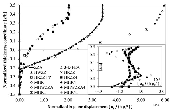
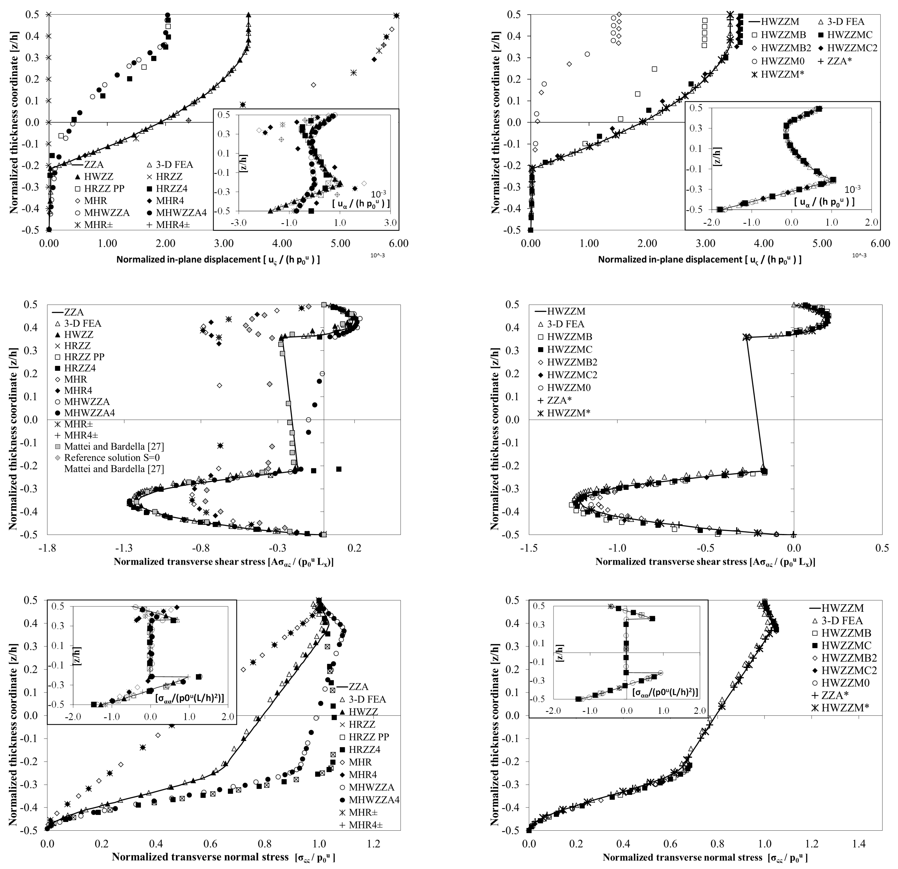
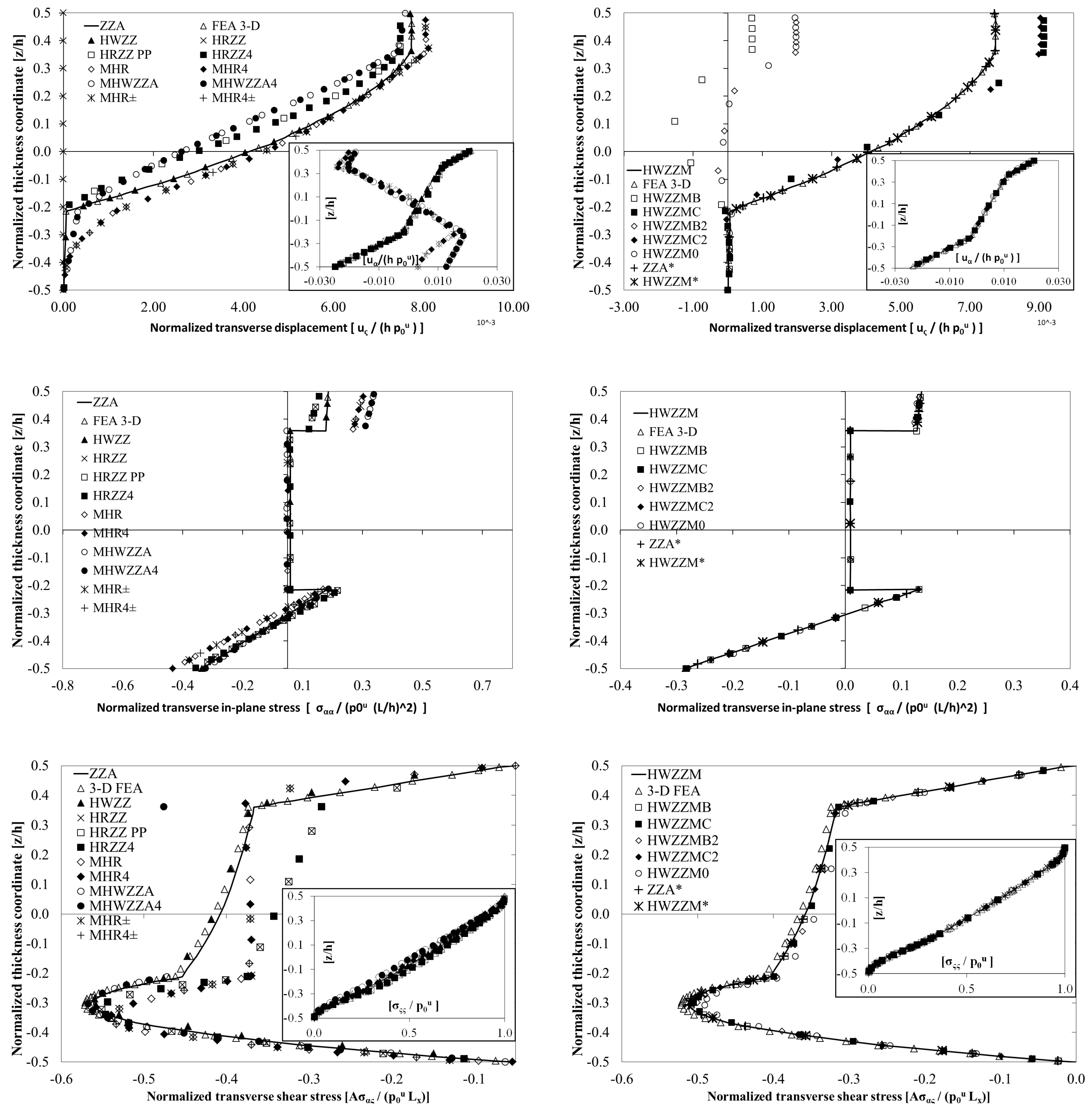
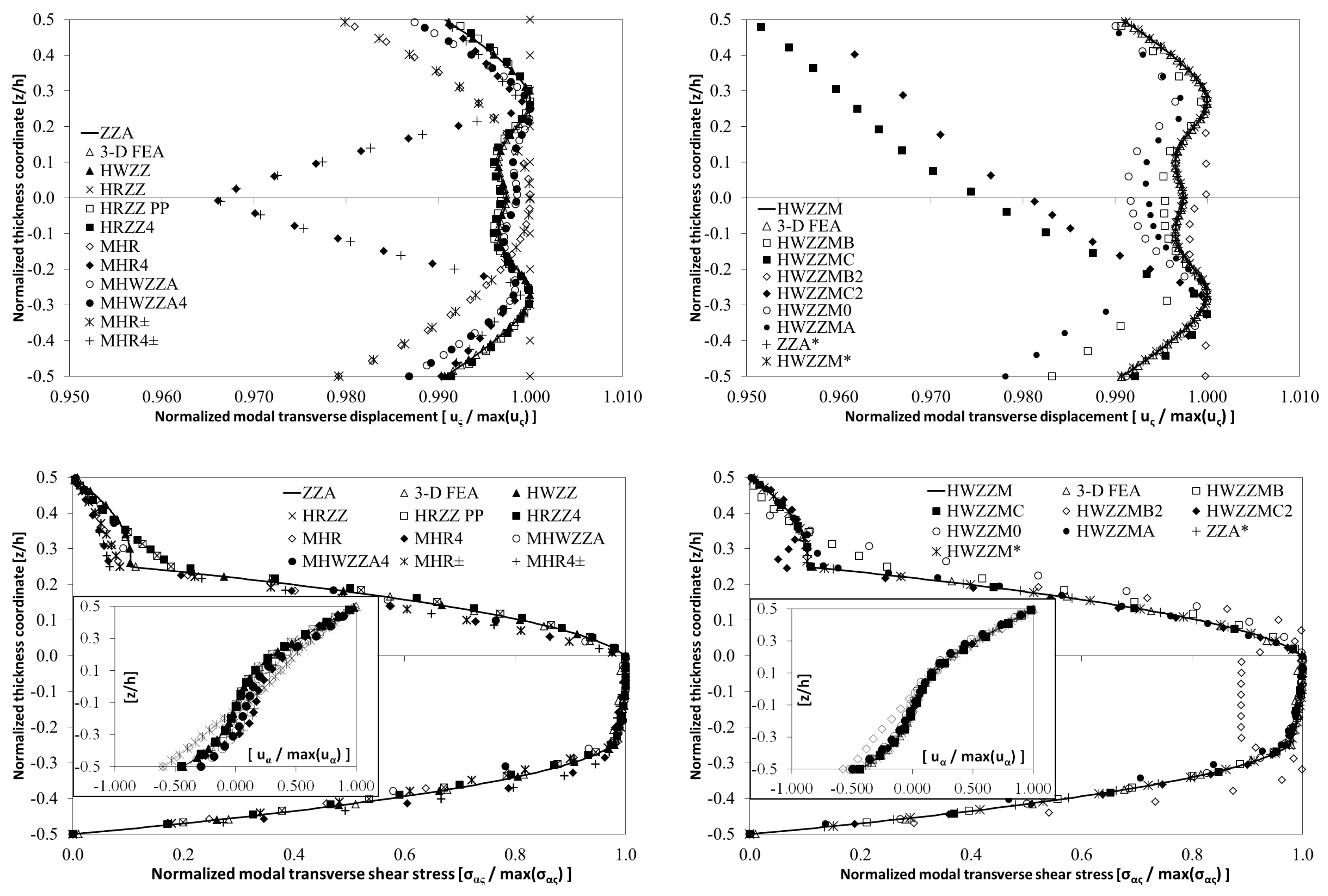
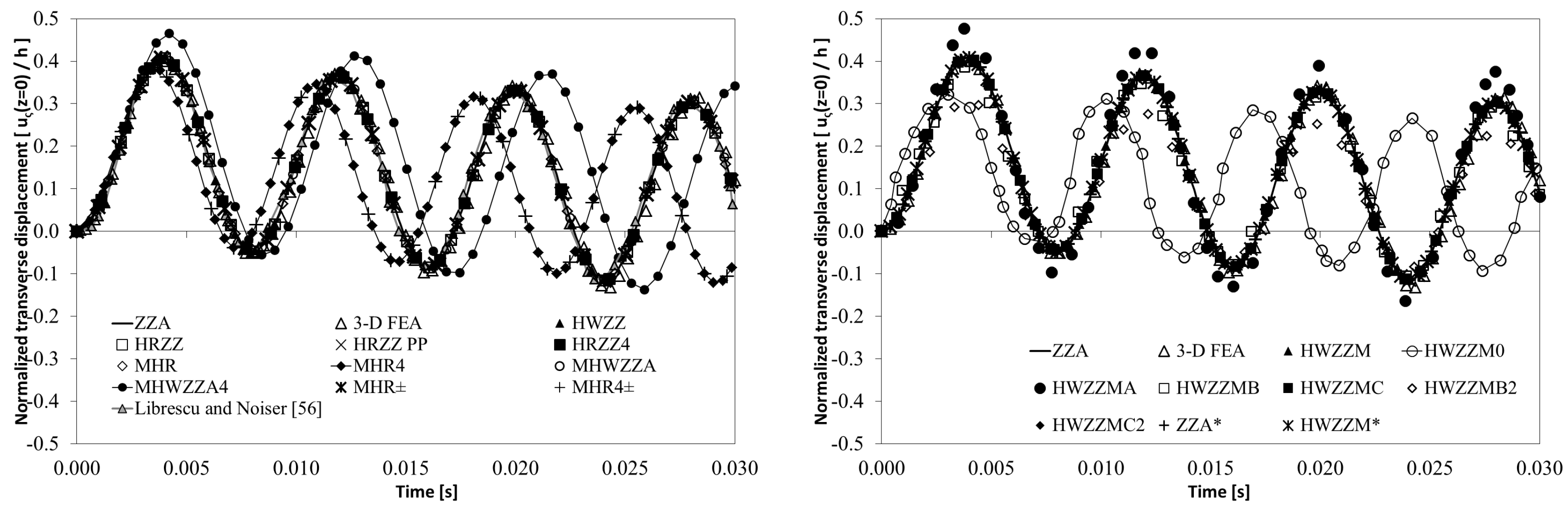
Table 1.
Acronyms.
| Acronym | Meaning | Acronym | Meaning |
|---|---|---|---|
| 3D FEA | Mixed solid 3D elements (Ref. [48]). | MHR | HR mixed theory with Murakami’s zig-zag function (see Section 4.1, Ref. [47]). |
| DL | Discrete-layer theories. | MHR± | MHR with slope defined on a physical basis (see Section 4.1). |
| DZZ | Di Sciuva’s zig-zag theory (Ref. [22]). | MHR4 | MHR with fourth-order polynomial transverse displacement (see Section 4.2, Ref. [47]). |
| EFSDT | Theory from Ref. [49]. | MHR4± | MHR4 with slope defined on a physical basis (see Section 4.2). |
| EHSDT | Theory from Ref. [49]. | MHWZZA | Modified HWZZ theory, type A (see Section 4.2, Ref. [47]). |
| ESL | Equivalent single-layer. | MHWZZA4 | Modified MHWZZA theory, with fourth-order piecewise polynomial transverse displacement (see Section 4.2, Ref. [47]). |
| FSDT | First-order shear deformation theory. | MZZ | Murakami’s like zig-zag theory (Ref. [23]). |
| HR | Hellinger–Reissner variational theorem. | PVW | Principle of virtual work. |
| HRZZ | HR zig-zag theory (see Section 4.3, Ref. [47]). | RFSDT | Theory from Ref. [50]. |
| HRZZ PP | Post-processed HRZZ (see Section 4.3). | RHQ40 | Finite element from Ref. [50]. |
| HRZZ4 | HRZZ with fourth-order polynomial transverse displacement (see Section 4.3, Ref. [47]). | RHSDT | Theory from Ref. [50]. |
| HSDT | Higher-order shear deformation theory. | RZT | Theory from Ref. [42]. |
| HW | Hu–Washizu variational theorem. | SEUPT | Strain energy update technique (Ref. [29]). |
| HWg | Hu–Washizu canonical functional (see Section 2.1). | TOT | Theory from Ref. [5]. |
| HWZZ | HW zig-zag mixed theory (see Section 3.2, Ref. [47]). | ZIGT | Theory from Ref. [5]. |
| HWZZM | Modified HWZZ theory, type M, (see Section 3.3.1). | ZZ | Plate theories with zig-zag contributions. |
| HWZZM* | Modified HWZZ theory, type M*, (see Section 3.3.2). | ZZA | Zig-zag adaptive theory (see Section 3.1, Ref. [29]). |
| HWZZM(†) | Modified HWZZM theories, type † (see Section 3.3.2.2). | ZZA* | Modified ZZA theory (see Section 3.1.1). |
† = A, B, B2, C, C2, 0 (variants of theory).
Table 2.
Trial functions.
| Case | Expansion Order | Mesh (xa·yb·zh) (+) | Trial Function |
|---|---|---|---|
| b1 | 1 | 16·2·60 | |
| b2 | 1 | 16·2·60 | |
| b3 | 1 | 16·2·60 | |
| e1 | 5 | 16·2·60 | |
| g | 3 | 16·2·60 | |
| c1 | 1 | 10·10·28 | |
| c2 | 1 | 10·10·28 | |
| d1 | 1 | 10·10·28 | |
| d2 | 1 | 10·10·28 | |
| e3 | 6 | 10·10·28 | |
| h | 5 | 10·10·28 | |
| i1 | 11 | 10·10·28 | |
| i2 | 11 | 10·10·28 | |
| i3 | 11 | 10·10·28 | |
| a1 | 9 | 16·2·60 | |
| a2 | 9 | 16·2·60 | |
| d2 | 4 | 10·10·28 | |
| e2 | 10 | 10·10·28 | |
| f | 6 | 10·10·28 |
(+) A uniform mesh is used; xa and yb represent the number of elements in x and y directions, respectively, zh is the number of elements across the thickness.
Table 3.
Data of cases.
| Case | Lay-Up | Layer Thickness | Material | BCS | Lx/h | Ly/Lx |
|---|---|---|---|---|---|---|
| a1 [27] | [0/0/0] | [(2h/7)/(4h/7)/(h/7)] | [n/n/n] | CS | 5.714 | - |
| a2 | [0/0/0] | [(2h/7)/(4h/7)/(h/7)] | [n/n/n] | CS | 20 | - |
| b1 [49] | [0/90/0] | [h/3]3 | [p]3 | SS | 10 | - |
| b2 [49] | [0/90/0/90] | [0.25h]4 | [p]4 | SS | 10 | - |
| b3 [49] (†) | [0/0/0] | [0.1h/0.8h/0.1h] | [p/mc/p] | SS | 4, 10, 20 | - |
| c1 [4] | [0/90/0/90] | [0.25h]4 | [a]4 | SSSS | 5 | 1 |
| c2 [4] | [90/0/90/0] | [0.25h]4 | [b]4 | SSSS | 10/3 | 1 |
| d1 [5] | [0/90/0] | [h/3]3 | [c]3 | SSSS | 4, 10, 20, 30, 50, 100 | 1 |
| d2 [50] | [0/90/0] | [h/3]3 | [c]3 | SSSS, CCCC, CSCS | 10 | 1 |
| e1 [5] | [0/90/0] | [0.25h/0.5h/0.25h] | [d]3 | SFSF | 5, 10, 20 | - |
| e2 [52] | [0/90/0] | [h/3]3 | [e]3 | CCCC | 10 | 1 |
| e3 [4] | [0/90/0/0/90] | [(h/24)2/(5h/12)]S | [f2/g]S | SSSS | 10 | 1 |
| f [53] | [0/90] | [h/2]2 | [h]2 | SS | 10 | 0.1 |
| g (*†) | [0]8 | [0.025h/0.05h/0.125h/0.3h]S | [m2/m1/m2/m3]S | SS | 5 | - |
| h (*†) | [0/90/0/0/90] | [(h/24)2/(5h/12)]S | [l1/l2/g/l1/l2] | SSSS | 5 | 1 |
| i1 [54] | [(45/−45)2/45/0]S | [(0.381mm)5/(12.7mm)]S | [o15/o2]S | SSSS | 20.8696 | 1 |
| i2 [55] | [0/90/0] | [(h/4)/(h/2)/(h/4)] | [q]3 | SSSS | 14.941 | 1 |
| i3 (*†) | [(0/90)2/02]S | [(0.381mm)5/(12.7mm)]S | [o15/o2/o3/o15] | SSSS | 10 | 1 |
* Transverse anisotropy; † Strong layerwise effects; (BCS: boundary conditions name; SS simply supported, C clamped).
Table 4.
Mechanical Properties.
| Material Name | a | b | c | d | e | f | g | h | l1 | l2 | m1 | m2 | m3 | mc | n [iso] | o1 | o2 | o3 | p | q |
|---|---|---|---|---|---|---|---|---|---|---|---|---|---|---|---|---|---|---|---|---|
| E1 [GPa] | M1 | 30E2 | 25E2 | 181 | 40E2 | 131 | 6.89 × 10⁻³ | 25E2 | 33.5 | 139 | 1 | 33 | 0.05 | 0.1 | - | 206.84 | 0.138 | 0.0138 | 172.4 | 132.4 |
| E2 [GPa] | - | - | - | 10.3 | - | 10.34 | 6.89 × 10⁻³ | - | 8 | 3.475 | 1 | 1 | 0.05 | 0.1 | - | 5.171 | 0.138 | 0.0138 | 6.9 | 10.8 |
| E3 [GPa] | E2 | E2 | E2 | 10.3 | E2 | 10.34 | 6.89 × 10⁻³ | E2 | 8 | 3.475 | 1 | 1 | 0.02 | 0.1 | M2 | 5.171 | 0. 138 | 0. 0138 | 6.9 | 10.8 |
| G12 [GPa] | 0.6E2 | 0.6E2 | 0.5E2 | 7.17 | 0.6E2 | 6.205 | 3.45 × 10⁻³ | 0.5E2 | 2.26 | 1.7375 | 0.02 | 8 | 0.0217 | 0.04 | - | 2.551 | 0.1027 | 0.01027 | 3.45 | 5.6 |
| G13 [GPa] | 0.6E2 | 0.6E2 | 0.5E2 | 7.17 | 0.6E2 | 6.895 | 3.45 × 10⁻³ | 0.2E2 | 2.26 | 1.7375 | 0.02 | 8 | 0.0217 | 0.04 | - | 2.551 | 0.1027 | 0.01027 | 3.45 | 5.6 |
| G23 [GPa] | 0.5E2 | 0.5E2 | 0.2E2 | 2.87 | 0.5E2 | 6.895 | 3.45 × 10⁻³ | 0.2E2 | 3 | 0.695 | 0.02 | 8 | 0.0217 | 0.04 | - | 2.551 | 0.06205 | 0.006205 | 1.38 | 5.6 |
| υ12 | 0.25 | 0.25 | 0.25 | 0.25 | 0.25 | 0.22 | 0 | 0.25 | 0.35 | 0.25 | 0.25 | 0.25 | 0.15 | 0.25 | 0.33 | 0.25 | 0.35 | 0.35 | 0.25 | 0.24 |
| υ13 | 0.25 | 0.25 | 0.25 | 0.25 | 0.25 | 0.22 | 0 | 0.25 | 0.35 | 0.25 | 0.25 | 0.25 | 0.15 | 0.25 | 0.33 | 0.25 | 0.35 | 0.35 | 0.25 | 0.24 |
| υ23 | 0.25 | 0.25 | 0.25 | 0.33 | 0.25 | 0.49 | 0 | 0.25 | 0.33 | 0.25 | 0.25 | 0.25 | 0.15 | 0.25 | 0.33 | 0.25 | 0.02 | 0.02 | 0.25 | 0.24 |
| Density [kg/m3] | ρ | ρ | ρ | 1587 | ρ | 1627 | 97 | ρ | 1627 | 1627 | 1558.35 | 1558.35 | 16.3136 | ρ | ρ | 1558.35 | 16.3136 | 16.3136 | ρ | 1443 |
M1 E1/E2 = 3, 10, 20, 30, 40; M2 Eu/El = 1.6, Eu/Ec = 166.66; [iso] = isotropic E1 = E2 = E3 G12 = G13 = G23.
Table 5.
Normalization of displacements, stresses and frequencies.
| Case | Normalization |
|---|---|
| a1 | |
| a2 | |
| b1 b2 b3 | |
| c1 | |
| c2 | |
| d1 d2 | |
| e1 | |
| e2 | |
| e3 | |
| f | |
| g | |
| h | |
| i1 i2 | |
| i3 | , |
Table 6.
Normalized fundamental frequencies, cases b1 and b2.
| Theory | 0/90/0 (b1) | 0/90/0/90 (b2) | Theory | 0/90/0 (b1) | 0/90/0/90 (b2) |
|---|---|---|---|---|---|
| 3D [49] | 0.1462 | 0.1095 | HWZZMC | 0.1463 | 0.1095 |
| EFSDT [49] | 0.1448 | 0.1125 | HWZZMC2 | 0.1465 | 0.1095 |
| EHSDT [49] | 0.1460 | 0.1090 | HWZZM0 | 0.1550 | 0.1220 |
| HSDT [49] | 0.1505 | 0.1139 | HRZZ | 0.1462 | 0.1094 |
| FSDT [49] | 0.1616 | 0.1186 | HRZZ4 | 0.1462 | 0.1095 |
| 3D FEA [48] | 0.1464 | 0.1096 | MHWZZA | 0.1460 | 0.1095 |
| ZZA | 0.1463 | 0.1095 | MHWZZA4 | 0.1461 | 0.1094 |
| ZZA* | 0.1463 | 0.1095 | MHR | 0.1463 | 0.1115 |
| HWZZ | 0.1463 | 0.1095 | MHR4 | 0.1463 | 0.1162 |
| HWZZM | 0.1463 | 0.1095 | MHR± | 0.1463 | 0.1115 |
| HWZZM* | 0.1463 | 0.1095 | MHR4± | 0.1463 | 0.1162 |
| HWZZMA | 0.2499 | 0.1130 | HSDT | 0.1511 | 0.1157 |
| HWZZMB | 0.2199 | 0.1095 | FSDT | 0.1565 | 0.1162 |
| HWZZMB2 | 0.1518 | 0.1124 |
Table 7.
Normalized fundamental frequencies, case b3.
| Lx/h | 4 | 10 | 20 | Lx/h | 4 | 10 | 20 |
|---|---|---|---|---|---|---|---|
| 3D [49] | 0.1011 | 0.0343 | 0.0155 | HWZZMC | 0.1017 | 0.0343 | 0.0156 |
| EFSDT [49] | 0.0848 | 0.0332 | 0.0153 | HWZZMC2 | 0.1017 | 0.0343 | 0.0155 |
| EHSDT [49] | 0.0972 | 0.0341 | 0.0155 | HWZZM0 | 0.1016 | 0.0343 | 0.0155 |
| FSDT [49] | 0.3325 | 0.1005 | 0.0316 | HRZZ | 0.0992 | 0.0342 | 0.0155 |
| 3D FEA [48] | 0.1011 | 0.0343 | 0.0155 | HRZZ4 | 0.0995 | 0.0342 | 0.0155 |
| ZZA | 0.1015 | 0.0343 | 0.0155 | MHWZZA | 0.1107 | 0.0373 | 0.0170 |
| ZZA* | 0.1015 | 0.0343 | 0.0155 | MHWZZA4 | 0.1083 | 0.0374 | 0.0170 |
| HWZZ | 0.1015 | 0.0343 | 0.0155 | MHR | 0.1015 | 0.0343 | 0.0155 |
| HWZZM | 0.1015 | 0.0343 | 0.0155 | MHR4 | 0.1015 | 0.0343 | 0.0155 |
| HWZZM* | 0.1015 | 0.0343 | 0.0155 | MHR± | 0.1015 | 0.0343 | 0.0155 |
| HWZZMA | 0.1250 | 0.0357 | 0.0159 | MHR4± | 0.1015 | 0.0343 | 0.0155 |
| HWZZMB | 0.1019 | 0.0343 | 0.0155 | HSDT | 0.1384 | 0.0503 | 0.0213 |
| HWZZMB2 | 0.1016 | 0.0343 | 0.0155 | FSDT | 0.3055 | 0.0956 | 0.0310 |
Table 8.
Normalized fundamental frequencies, case c1.
| Theory | E1/E2 = 3 | 10 | 20 | 30 | 40 |
|---|---|---|---|---|---|
| Exact [4] | 2.6182 | 3.2578 | 3.7622 | 4.0660 | 4.2719 |
| Zhen and Wanji [4] | 2.6127 | 3.2513 | 3.7523 | 4.0532 | 4.2568 |
| Matsunaga [56] | 2.6021 | 3.2380 | 3.7400 | 4.0425 | 4.2477 |
| 3D FEA [48] | 2.6118 | 3.2492 | 3.7500 | 4.0509 | 4.2546 |
| ZZA | 2.6026 | 3.2387 | 3.7406 | 4.0430 | 4.2481 |
| ZZA* | 2.6026 | 3.2387 | 3.7406 | 4.0430 | 4.2481 |
| HWZZ | 2.6026 | 3.2387 | 3.7406 | 4.0430 | 4.2481 |
| HWZZM | 2.6026 | 3.2387 | 3.7406 | 4.0430 | 4.2481 |
| HWZZM* | 2.6026 | 3.2387 | 3.7406 | 4.0430 | 4.2481 |
| HWZZMA | 2.6158 | 3.2591 | 3.7664 | 4.0716 | 4.2783 |
| HWZZMB | 2.6121 | 3.2529 | 3.7572 | 4.0603 | 4.2653 |
| HWZZMB2 | 3.1157 | 4.3980 | 5.7265 | 6.7186 | 7.4660 |
| HWZZMC | 2.6064 | 3.2468 | 3.7537 | 4.0601 | 4.2681 |
| HWZZMC2 | 2.6277 | 3.3004 | 3.8541 | 4.1970 | 4.4252 |
| HWZZM0 | 2.8890 | 3.4550 | 3.9188 | 4.2047 | 4.4024 |
| HRZZ | 2.5977 | 3.2289 | 3.7250 | 4.0230 | 4.2247 |
| HRZZ4 | 2.5980 | 3.2293 | 3.7255 | 4.0238 | 4.2256 |
| MHWZZA | 2.0844 | 4.0468 | 3.3020 | 3.1347 | 2.9820 |
| MHWZZA4 | 2.0639 | 4.0052 | 3.2626 | 3.1124 | 2.9785 |
| MHR | 2.6101 | 3.3696 | 4.1243 | 4.6940 | 5.1627 |
| MHR4 | 2.6265 | 3.3970 | 4.1616 | 4.7389 | 5.2142 |
| MHR± | 2.6038 | 3.2915 | 3.9165 | 4.3440 | 4.6645 |
| MHR4± | 2.6312 | 3.3774 | 4.0187 | 4.4254 | 4.7118 |
| HSDT | 2.6003 | 3.2781 | 3.8505 | 4.2139 | 4.4686 |
| FSDT | 2.5986 | 3.2836 | 3.8651 | 4.2342 | 4.4919 |
Table 9.
Normalized fundamental frequencies (NFQ), case c2.
| c2 | NFQ | Theory | NFQ | Theory | NFQ |
|---|---|---|---|---|---|
| 3D FEA [48] | 0.7041 | HWZZMB2 | 0.7268 | MHWZZA4 | 0.7652 |
| ZZA | 0.7044 | HWZZMC | 0.7043 | MHR | 0.9394 |
| ZZA* | 0.7044 | HWZZMC2 | 0.7199 | MHR4 | 0.7596 |
| HWZZ | 0.7044 | HWZZM0 | 0.7047 | MHR± | 0.7609 |
| HWZZM | 0.7044 | HRZZ | 0.6860 | MHR4± | 0.7674 |
| HWZZM* | 0.7044 | HRZZ4 | 0.6855 | HSDT | 0.7432 |
| HWZZMA | 0.7094 | MHWZZA | 0.7505 | FSDT | 0.7451 |
| HWZZMB | 0.7084 |
Table 10.
Normalized fundamental frequencies, case d1.
| Lx/h | 4 | 10 | 20 | 30 | 50 | 100 |
|---|---|---|---|---|---|---|
| RFSDT [50] | 7.1630 | 11.7000 | 14.0120 | 14.6450 | 15.0090 | 15.1720 |
| RHSDT [50] | 7.0270 | 11.4620 | 13.8880 | 14.5790 | 14.9830 | 15.1650 |
| 3D FEA [48] | 6.8436 | 11.4306 | 13.9231 | 14.6593 | 15.0696 | 15.2550 |
| ZZA | 6.9254 | 11.4583 | 13.8889 | 14.5800 | 14.9833 | 15.1654 |
| ZZA* | 6.9254 | 11.4583 | 13.8889 | 14.5800 | 14.9833 | 15.1654 |
| HWZZ | 6.9254 | 11.4583 | 13.8889 | 14.5800 | 14.9833 | 15.1654 |
| HWZZM | 6.9254 | 11.4583 | 13.8889 | 14.5800 | 14.9833 | 15.1654 |
| HWZZM* | 6.9254 | 11.4583 | 13.8889 | 14.5800 | 14.9833 | 15.1654 |
| HWZZMA | 9.0597 | 14.2814 | 15.0815 | 15.0371 | 15.0748 | 15.1730 |
| HWZZMB | 8.3007 | 15.9403 | 18.0802 | 15.8433 | 15.1554 | 15.1760 |
| HWZZMB2 | 7.6251 | 12.6836 | 13.9248 | 14.5871 | 14.9843 | 15.1655 |
| HWZZMC | 6.9999 | 11.4660 | 13.8897 | 14.5802 | 14.9834 | 15.1654 |
| HWZZMC2 | 7.1409 | 11.4823 | 13.8915 | 14.5806 | 14.9834 | 15.1654 |
| HWZZM0 | 7.2859 | 12.5356 | 17.7326 | 21.7236 | 27.4298 | 33.3973 |
| HRZZ | 6.3896 | 11.4502 | 13.8862 | 14.5787 | 14.9828 | 15.1653 |
| HRZZ4 | 6.9104 | 11.4569 | 13.8888 | 14.5799 | 14.9833 | 15.1654 |
| MHWZZA | 9.9632 | 9.1000 | 12.3099 | 13.8952 | 14.7385 | 15.1043 |
| MHWZZA4 | 9.9815 | 9.1054 | 12.3100 | 13.8952 | 14.7385 | 15.1043 |
| MHR | 6.9913 | 11.4647 | 13.8896 | 14.5802 | 14.9834 | 15.1654 |
| MHR4 | 7.4725 | 11.6644 | 14.0961 | 14.7437 | 15.0712 | 15.1924 |
| MHR± | 6.9913 | 11.4647 | 13.8896 | 14.5802 | 14.9834 | 15.1654 |
| MHR4± | 7.4725 | 11.6644 | 14.0961 | 14.7437 | 15.0712 | 15.1924 |
| HSDT | 7.1160 | 11.7900 | 14.0600 | 14.6700 | 15.0190 | 15.1750 |
| FSDT | 7.4130 | 12.1630 | 14.2300 | 14.7570 | 15.0530 | 15.1830 |
Table 11.
Normalized fundamental frequencies, case d2.
| Theory | SSSS | CSCS | CCCC | Theory | SSSS | CSCS | CCCC |
|---|---|---|---|---|---|---|---|
| RHQ40 [50] | 11.4000 | 15.9550 | 17.4810 | HWZZM0 | 12.5356 | 17.1426 | 18.2727 |
| 3D FEA [48] | 11.4306 | 15.3895 | 16.6658 | HRZZ | 11.4502 | 16.1304 | 17.5659 |
| ZZA | 11.4583 | 15.1875 | 16.4575 | HRZZ4 | 11.4569 | 16.1481 | 17.6134 |
| ZZA* | 11.4583 | 15.1875 | 16.4575 | MHWZZA | 9.1000 | 6.0313 | 20.8865 |
| HWZZ | 11.4583 | 15.1875 | 16.4575 | MHWZZA4 | 9.1054 | 6.3368 | 21.0304 |
| HWZZM | 11.4583 | 15.1875 | 16.4575 | MHR | 11.4647 | 16.6145 | 18.0505 |
| HWZZM* | 11.4583 | 15.1875 | 16.4575 | MHR4 | 11.6644 | 16.9713 | 18.4802 |
| HWZZMA | 14.2814 | 17.4395 | 19.2037 | MHR± | 11.4647 | 16.6145 | 18.0505 |
| HWZZMB | 15.9403 | 20.8031 | 20.9520 | MHR4± | 11.6644 | 16.9713 | 18.4802 |
| HWZZMB2 | 12.6836 | 16.8409 | 17.8968 | HSDT | 11.7900 | 17.4157 | 18.5237 |
| HWZZMC | 11.4660 | 14.5666 | 14.7679 | FSDT | 12.1630 | 16.4436 | 17.5603 |
| HWZZMC2 | 11.4823 | 16.5033 | 18.0240 |
Table 12.
Normalized fundamental frequencies, case e1.
| Lx/h = 5 | Mode 1 | Mode 2 | Mode 3 | Mode 4 | Mode 5 |
|---|---|---|---|---|---|
| Exact [5] | 6.8060 | 16.5150 | 26.6880 | 37.2550 | 48.0350 |
| Zhen and Wanji [4] | 6.8161 | 16.6154 | 27.4212 | 39.8230 | 54.1984 |
| ZIGT [5] | 6.8128 | 16.7297 | 27.8623 | 40.9060 | 56.1529 |
| TOT [5] | 6.9762 | 16.8783 | 27.1417 | 38.1864 | 50.3407 |
| FSDT [5] | 7.4458 | 18.2491 | 28.7697 | 41.1668 | 49.2839 |
| 3D FEA [48] | 6.8115 | 16.5343 | 26.7475 | 37.3746 | 48.3752 |
| ZZA | 6.8116 | 16.5253 | 26.7123 | 37.2801 | 49.1224 |
| ZZA* | 6.8116 | 16.5253 | 26.7123 | 37.2801 | 49.1224 |
| HWZZ | 6.8116 | 16.5253 | 26.7123 | 37.2801 | 49.1224 |
| HWZZM | 6.8116 | 16.5253 | 26.7123 | 37.2801 | 49.1224 |
| HWZZM* | 6.8116 | 16.5253 | 26.7123 | 37.2801 | 49.1224 |
| HWZZMA | 6.8351 | 17.5435 | 27.2260 | 39.0876 | 55.4790 |
| HWZZMB | 6.8136 | 16.5504 | 26.8150 | 37.5666 | 49.9111 |
| HWZZMB2 | 6.8165 | 16.5876 | 26.9680 | 37.9747 | 50.6078 |
| HWZZMC | 6.8153 | 16.5795 | 26.9446 | 37.9232 | 50.5189 |
| HWZZMC2 | 6.8150 | 16.5769 | 26.9400 | 37.9217 | 50.5219 |
| HWZZM0 | 6.8136 | 16.6907 | 27.1274 | 38.0196 | 50.2967 |
| HRZZ | 6.8140 | 16.5026 | 26.6062 | 37.0322 | 48.7296 |
| HRZZ4 | 6.8080 | 16.4870 | 26.6057 | 37.1091 | 48.9903 |
| MHWZZA | 6.4175 | 15.5732 | 25.2021 | 35.8711 | 46.9424 |
| MHWZZA4 | 6.8271 | 16.5673 | 26.8199 | 37.4702 | 49.4131 |
| MHR | 6.8198 | 16.6463 | 27.2066 | 38.5180 | 51.6381 |
| MHR4 | 6.8202 | 16.6614 | 27.2706 | 38.6497 | 51.8742 |
| MHR± | 6.8198 | 16.6463 | 27.2066 | 38.5180 | 51.6381 |
| MHR4± | 6.8202 | 16.6614 | 27.2706 | 38.6497 | 51.8742 |
| HSDT | 6.9828 | 16.8828 | 27.1485 | 38.1713 | 51.2504 |
| FSDT | 7.4237 | 18.1565 | 28.5888 | 38.7856 | 50.1428 |
Table 13.
Normalized fundamental frequencies, case e1.
| Lx/h = 10 | Mode 1 | Mode 2 | Mode 3 | Mode 4 | Mode 5 |
|---|---|---|---|---|---|
| Exact [5] | 9.3434 | 27.2240 | 46.4190 | 66.0580 | 86.1690 |
| Zhen and Wanji [4] | 9.3748 | 27.3267 | 46.6609 | 66.6898 | 87.7990 |
| ZIGT [5] | 9.3434 | 27.2512 | 46.6511 | 66.9168 | 88.4094 |
| TOT [5] | 9.4742 | 27.9046 | 47.6259 | 67.5113 | 87.7200 |
| FSDT [5] | 9.7639 | 29.7831 | 51.4787 | 72.9941 | 94.1827 |
| 3D FEA [48] | 9.3534 | 27.1962 | 46.4747 | 66.3024 | 86.8487 |
| ZZA | 9.3556 | 27.2463 | 46.4492 | 66.0544 | 87.6999 |
| ZZA* | 9.3556 | 27.2463 | 46.4492 | 66.0544 | 87.6999 |
| HWZZ | 9.3556 | 27.2463 | 46.4492 | 66.0544 | 87.6999 |
| HWZZM | 9.3556 | 27.2463 | 46.4492 | 66.0544 | 87.6999 |
| HWZZM* | 9.3556 | 27.2463 | 46.4492 | 66.0544 | 87.6999 |
| HWZZMA | 9.3634 | 27.3403 | 46.9501 | 70.1202 | 89.1944 |
| HWZZMB | 9.3561 | 27.2544 | 46.4856 | 66.1550 | 88.2045 |
| HWZZMB2 | 9.3568 | 27.2661 | 46.5389 | 66.3042 | 88.5122 |
| HWZZMC | 9.3561 | 27.2612 | 46.5239 | 66.2718 | 88.4563 |
| HWZZMC2 | 9.3560 | 27.2598 | 46.5189 | 66.2615 | 88.4411 |
| HWZZM0 | 9.3562 | 27.4362 | 46.8354 | 66.7382 | 89.0772 |
| HRZZ | 9.3589 | 27.2560 | 46.4346 | 65.9635 | 87.7726 |
| HRZZ4 | 9.3549 | 27.2320 | 46.3866 | 65.9012 | 87.7148 |
| MHWZZA | 7.4987 | 20.7918 | 42.6638 | 65.0068 | 87.5899 |
| MHWZZA4 | 9.3733 | 27.3067 | 46.5481 | 66.2214 | 88.3184 |
| MHR | 9.3577 | 27.2792 | 46.6134 | 66.5364 | 89.1480 |
| MHR4 | 9.3577 | 27.2808 | 46.6293 | 66.5962 | 89.3332 |
| MHR± | 9.3577 | 27.2792 | 46.6134 | 66.5364 | 89.1480 |
| MHR4± | 9.3577 | 27.2808 | 46.6293 | 66.5962 | 89.3332 |
| HSDT | 9.4832 | 27.9312 | 47.6368 | 67.4822 | 89.5987 |
| FSDT | 9.7608 | 29.6950 | 51.2648 | 72.5723 | 95.7078 |
Table 14.
Normalized fundamental frequencies, case e1.
| Lx/h = 20 | Mode 1 | Mode 2 | Mode 3 | Mode 4 | Mode 5 |
|---|---|---|---|---|---|
| Exact [5] | 10.6400 | 37.3740 | 71.7440 | 108.8900 | 147.0400 |
| Zhen and Wanji [4] | 10.6897 | 37.6810 | 72.6193 | 110.5376 | 149.6296 |
| ZIGT [5] | 10.6400 | 37.3740 | 71.7440 | 108.9989 | 147.4811 |
| TOT [5] | 10.6932 | 37.8972 | 73.2506 | 111.6123 | 150.8630 |
| FSDT [5] | 10.7890 | 39.0558 | 77.0531 | 119.1257 | 162.4792 |
| 3D FEA [48] | 10.6527 | 37.3755 | 71.5020 | 108.9389 | 147.0909 |
| ZZA | 10.6575 | 37.4222 | 71.8164 | 108.9263 | 149.6777 |
| ZZA* | 10.6575 | 37.4222 | 71.8164 | 108.9263 | 149.6777 |
| HWZZ | 10.6575 | 37.4222 | 71.8164 | 108.9263 | 149.6777 |
| HWZZM | 10.6575 | 37.4222 | 71.8164 | 108.9263 | 149.6777 |
| HWZZM* | 10.6575 | 37.4222 | 71.8164 | 108.9263 | 149.6777 |
| HWZZMA | 10.6601 | 37.4536 | 71.9498 | 109.2996 | 150.7192 |
| HWZZMB | 10.6577 | 37.4243 | 71.8267 | 108.9586 | 149.7543 |
| HWZZMB2 | 10.6580 | 37.4272 | 71.8418 | 109.0057 | 149.8559 |
| HWZZMC | 10.6575 | 37.4246 | 71.8334 | 108.9862 | 149.8207 |
| HWZZMC2 | 10.6575 | 37.4242 | 71.8312 | 108.9804 | 149.8098 |
| HWZZM0 | 10.6583 | 37.6355 | 72.2589 | 109.6109 | 150.6415 |
| HRZZ | 10.6589 | 37.4357 | 71.8491 | 108.9650 | 149.2023 |
| HRZZ4 | 10.6574 | 37.4197 | 71.7993 | 108.8690 | 149.2281 |
| MHWZZA | 10.5652 | 37.1202 | 71.2611 | 108.0743 | 146.5888 |
| MHWZZA4 | 10.6719 | 37.4952 | 71.9809 | 109.1660 | 148.0695 |
| MHR | 10.6581 | 37.4306 | 71.8579 | 109.0565 | 150.0877 |
| MHR4 | 10.6581 | 37.4307 | 71.8588 | 109.0624 | 150.1300 |
| MHR± | 10.6581 | 37.4306 | 71.8579 | 109.0565 | 150.0877 |
| MHR4± | 10.6581 | 37.4307 | 71.8588 | 109.0624 | 150.1300 |
| HSDT | 10.7061 | 37.9327 | 73.3318 | 111.6654 | 153.6012 |
| FSDT | 10.8047 | 39.0433 | 76.9153 | 118.7217 | 164.5034 |
Table 15.
Normalized fundamental frequencies, case e2.
| Theory | Mode 1 | Mode 2 | Mode 3 | Mode 4 | Mode 5 | Mode 6 | Mode 7 | Mode 8 |
|---|---|---|---|---|---|---|---|---|
| Liew [54] | 4.4470 | 6.6420 | 7.7000 | 9.1850 | 9.7380 | 11.3990 | 11.6440 | 12.4660 |
| Zhen and Wanji [4] | 4.5400 | 6.5240 | 8.1780 | 9.4730 | 9.4920 | 11.7690 | 12.3950 | 12.9040 |
| 3D FEA [48] | 4.4815 | 6.4637 | 7.9938 | 9.3025 | 9.3507 | 11.3722 | 11.5329 | 12.3221 |
| ZZA | 4.4682 | 6.5561 | 8.1065 | 9.3271 | 9.3371 | 11.1756 | 11.7574 | 12.1556 |
| ZZA* | 4.4682 | 6.5561 | 8.1065 | 9.3271 | 9.3371 | 11.1756 | 11.7574 | 12.1556 |
| HWZZ | 4.4682 | 6.5561 | 8.1065 | 9.3271 | 9.3371 | 11.1756 | 11.7574 | 12.1556 |
| HWZZM | 4.4682 | 6.5561 | 8.1065 | 9.3271 | 9.3371 | 11.1756 | 11.7574 | 12.1556 |
| HWZZM* | 4.4682 | 6.5561 | 8.1065 | 9.3271 | 9.3371 | 11.1756 | 11.7574 | 12.1556 |
| HWZZMA | 5.8520 | 7.5208 | 8.1724 | 10.4894 | 11.1722 | 11.2569 | 12.0353 | 13.1691 |
| HWZZMB | 4.9570 | 6.9202 | 8.1959 | 9.6129 | 10.7028 | 11.1675 | 11.9800 | 13.0014 |
| HWZZMB2 | 6.0808 | 7.7635 | 8.8739 | 10.0492 | 10.8949 | 11.2114 | 12.6851 | 13.2650 |
| HWZZMC | 4.4859 | 6.6243 | 8.1606 | 9.6488 | 9.8538 | 11.1884 | 11.8340 | 13.2442 |
| HWZZMC2 | 4.5001 | 6.6668 | 8.0939 | 9.6464 | 10.3489 | 11.1834 | 11.8285 | 13.6387 |
| HWZZM0 | 4.4380 | 6.4692 | 8.6268 | 9.6356 | 10.2157 | 11.1670 | 11.9858 | 12.6024 |
| HRZZ | 4.4780 | 6.5756 | 8.6593 | 9.0735 | 9.5258 | 10.9819 | 11.6335 | 12.1995 |
| HRZZ4 | 4.4923 | 6.5622 | 8.6120 | 9.4418 | 9.4418 | 10.9114 | 11.6410 | 12.2389 |
| MHWZZA | 5.7704 | 12.5575 | 12.8292 | 14.2568 | 15.3680 | 18.8049 | 21.7441 | 28.1598 |
| MHWZZA4 | 5.8917 | 11.1227 | 12.9126 | 14.1157 | 15.2158 | 18.6187 | 21.5288 | 27.8810 |
| MHR | 4.6236 | 6.4996 | 9.0278 | 9.5643 | 9.7380 | 12.2893 | 12.3381 | 14.5644 |
| MHR4 | 5.7578 | 10.8328 | 12.8328 | 14.3956 | 14.4156 | 19.1566 | 19.9439 | 20.5045 |
| MHR± | 4.6236 | 6.4996 | 9.0278 | 9.5643 | 9.7380 | 12.2893 | 12.3381 | 14.5644 |
| MHR4± | 5.7578 | 10.8328 | 12.8328 | 14.3956 | 14.4156 | 19.1566 | 19.9439 | 20.5045 |
| HSDT | 4.2424 | 6.4851 | 9.0818 | 9.6084 | 10.3515 | 11.5880 | 14.3931 | 13.3191 |
| FSDT | 4.1816 | 6.5979 | 8.5147 | 9.3171 | 10.2948 | 11.3770 | 11.5306 | 13.1945 |
Table 16.
Normalized fundamental frequencies, case e3.
| Theory | Mode 1 | Mode 2 | Mode 3 | Mode 4 | Mode 5 | Mode 6 |
|---|---|---|---|---|---|---|
| Zhen and Wanji [4] | 1.9445 | 3.3796 | 4.5914 | 5.5268 | 6.5128 | 8.4311 |
| 3D FEA [48] | 1.8497 | 3.2308 | 4.3091 | 5.2810 | 6.1583 | 7.7796 |
| ZZA | 1.8566 | 3.2341 | 4.3215 | 5.2778 | 6.1782 | 7.8258 |
| ZZA* | 1.8566 | 3.2341 | 4.3215 | 5.2778 | 6.1782 | 7.8258 |
| HWZZ | 1.8566 | 3.2341 | 4.3215 | 5.2778 | 6.1782 | 7.8258 |
| HWZZM | 1.8566 | 3.2341 | 4.3215 | 5.2778 | 6.1782 | 7.8258 |
| HWZZM* | 1.8566 | 3.2341 | 4.3215 | 5.2778 | 6.1782 | 7.8258 |
| HWZZMA | 2.9945 | 8.2464 | 13.0020 | 23.1893 | 27.6448 | 29.3959 |
| HWZZMB | 1.8699 | 3.2238 | 4.4780 | 6.4664 | 7.0973 | 8.4051 |
| HWZZMB2 | 2.5594 | 3.3902 | 4.4765 | 6.7477 | 7.1172 | 19.0397 |
| HWZZMC | 4.3268 | 3.2572 | 4.3669 | 5.3203 | 6.2311 | 7.8900 |
| HWZZMC2 | 1.8603 | 3.3297 | 4.4768 | 5.4447 | 6.3394 | 8.0418 |
| HWZZM0 | 3.0133 | 7.4920 | 10.3910 | 11.3215 | 15.1346 | 21.7804 |
| HRZZ | 1.8359 | 3.1546 | 4.1342 | 4.9488 | 5.6326 | 6.5177 |
| HRZZ4 | 1.8375 | 3.1628 | 4.1541 | 4.9832 | 5.6931 | 6.6864 |
| MHWZZA | 4.5991 | 6.3956 | 2.5602 | 2.9859 | 55.0032 | 35.4337 |
| MHWZZA4 | 4.5536 | 6.3323 | 2.5349 | 2.9563 | 54.4586 | 35.0828 |
| MHR | 13.9456 | 29.5039 | 41.6109 | 68.7426 | 65.8617 | 71.6472 |
| MHR4 | 13.9456 | 29.5039 | 41.6109 | 68.7426 | 65.8617 | 71.6472 |
| MHR± | 1.8542 | 3.2453 | 4.3281 | 5.2674 | 6.1564 | 7.7888 |
| MHR4± | 11.0690 | 14.1130 | 14.9723 | 15.2744 | 16.5324 | 18.4374 |
| HSDT | 6.5797 | 12.7968 | 14.5661 | 22.9323 | 26.7542 | 30.9263 |
| FSDT | 13.9752 | 31.0136 | 42.0946 | 51.7209 | 59.2477 | 72.5151 |
Table 17.
Normalized fundamental frequencies, case f.
| Theory | Mode 1 | Mode 2 | Mode 3 | Mode 4 |
|---|---|---|---|---|
| 3D FEA [53] | 5.7720 | 8.7220 | 17.8210 | 95.3190 |
| N = 3 (30 DOFS) [53] | 5.7976 | 8.8428 | 19.5380 | 98.1640 |
| 3D FEA [48] | 5.7769 | 8.7914 | 17.8705 | 95.3828 |
| ZZA | 5.7770 | 8.8424 | 17.7962 | 97.1215 |
| ZZA* | 5.7770 | 8.8424 | 17.7962 | 97.1215 |
| HWZZ | 5.7770 | 8.8424 | 17.7962 | 97.1215 |
| HWZZM | 5.7770 | 8.8424 | 17.7962 | 97.1215 |
| HWZZM* | 5.7770 | 8.8424 | 17.7962 | 97.1215 |
| HWZZMA | 5.7770 | 8.8424 | 17.7962 | 97.1215 |
| HWZZMB | 5.7770 | 8.8424 | 17.7962 | 97.1215 |
| HWZZMB2 | 5.7770 | 8.8424 | 17.7962 | 97.1215 |
| HWZZMC | 5.7770 | 8.8424 | 17.7962 | 97.1215 |
| HWZZMC2 | 5.7770 | 8.8424 | 17.7962 | 97.1215 |
| HWZZM0 | 5.7791 | 8.8522 | 17.7800 | 101.5429 |
| HRZZ | 5.7722 | 8.8389 | 18.4970 | 101.6298 |
| HRZZ4 | 5,7767 | 8,8087 | 18,4986 | 101,6402 |
| MHWZZA | 6.1101 | 9.8335 | 22.2173 | 99.8945 |
| MHWZZA4 | 5.8063 | 9.8330 | 22.2071 | 99.2816 |
| MHR | 5.8766 | 9.6492 | 20.5639 | 97.0202 |
| MHR4 | 5.8955 | 9.6492 | 20.2339 | 105.1698 |
| MHR± | 5.8766 | 9.6492 | 20.5639 | 97.0202 |
| MHR4± | 5.8955 | 9.6492 | 20.2339 | 105.1698 |
Table 18.
Normalized fundamental frequencies, case g.
| Theory | Mode 1 | Mode 2 | Mode 3 | Mode 4 | Mode 5 |
|---|---|---|---|---|---|
| 3D FEA [48] | 4.1785 | 10.4238 | 14.6587 | 16.4979 | 19.0105 |
| ZZA | 4.1788 | 10.4263 | 14.6864 | 16.5272 | 19.0239 |
| ZZA* | 4.1788 | 10.4263 | 14.6864 | 16.5272 | 19.0239 |
| HWZZ | 4.1788 | 10.4263 | 14.6864 | 16.5272 | 19.0239 |
| HWZZM | 4.1788 | 10.4263 | 14.6864 | 16.5272 | 19.0239 |
| HWZZM* | 4.1788 | 10.4263 | 14.6864 | 16.5272 | 19.0239 |
| HWZZMA | 14.6663 | 51.8295 | 82.2952 | 171.8208 | 89.6849 |
| HWZZMB | 4.2350 | 33.5909 | 91.3964 | 157.6279 | 68.3833 |
| HWZZMB2 | 4.3790 | 24.8306 | 91.5540 | 159.3091 | 58.0426 |
| HWZZMC | 4.1790 | 10.4292 | 14.6857 | 16.5275 | 19.1303 |
| HWZZMC2 | 4.1790 | 10.4288 | 14.6860 | 16.5276 | 19.0365 |
| HWZZM0 | 4.2300 | 11.5140 | 91.2793 | 157.4339 | 41.1479 |
| HRZZ | 4.1373 | 9.9206 | 88.7309 | 151.5792 | 16.6322 |
| HRZZ4 | 4.1380 | 9.9266 | 88.6647 | 151.2531 | 16.6531 |
| MHWZZA | 3.0776 | 5.0099 | 20.3131 | 29.1520 | 6.3628 |
| MHWZZA4 | 4.1977 | 11.3344 | 21.3343 | 24.6261 | 21.2708 |
| MHR | 15.2050 | 42.4682 | 77.9566 | 154.7082 | 70.0325 |
| MHR4 | 15.2011 | 42.2872 | 65.2275 | 65.4027 | 66.8219 |
| MHR± | 15.2050 | 42.4682 | 77.9566 | 154.7082 | 70.0325 |
| MHR4± | 15.0620 | 32.3678 | 17.9254 | 26.7157 | 57.4925 |
| HSDT | 14.1892 | 37.7022 | *** | *** | 61.7475 |
| FSDT | 16.3886 | 49.9499 | *** | *** | 87.0203 |
*** Not provided by the theory.
Table 19.
Normalized fundamental frequencies, case h.
| Theory | Mode 1 | Mode 2 | Mode 3 | Mode 4 | Mode 5 | Mode 6 |
|---|---|---|---|---|---|---|
| 3D FEA [48] | 1.6882 | 2.8796 | 3.4723 | 4.3033 | 4.6899 | 5.7441 |
| ZZA | 1.6898 | 2.8855 | 3.4777 | 4.3171 | 4.7030 | 5.7500 |
| ZZA* | 1.6898 | 2.8855 | 3.4777 | 4.3171 | 4.7030 | 5.7500 |
| HWZZ | 1.6898 | 2.8855 | 3.4777 | 4.3171 | 4.7030 | 5.7500 |
| HWZZM | 1.6898 | 2.8855 | 3.4777 | 4.3171 | 4.7030 | 5.7500 |
| HWZZM* | 1.6898 | 2.8855 | 3.4777 | 4.3171 | 4.7030 | 5.7500 |
| HWZZMA | 5.3141 | 7.2110 | 11.3333 | 19.3264 | 21.7117 | 46.2461 |
| HWZZMB | 1.7010 | 2.8913 | 3.5605 | 4.3693 | 4.7101 | 34.1888 |
| HWZZMB2 | 1.7651 | 4.7210 | 3.5473 | 5.0578 | 10.6544 | 34.7002 |
| HWZZMC | 1.6898 | 2.8855 | 3.4778 | 4.3171 | 4.7030 | 5.7500 |
| HWZZMC2 | 1.6898 | 2.8855 | 3.4778 | 4.3171 | 4.7030 | 5.7500 |
| HWZZM0 | 2.5169 | 5.6364 | 5.9019 | 8.8827 | 11.3106 | 34.3120 |
| HRZZ | 1.6823 | 2.8517 | 3.3940 | 4.1648 | 4.5907 | 34.3046 |
| HRZZ4 | 1.6821 | 2.8525 | 3.3965 | 4.1720 | 4.5948 | 34.1832 |
| MHWZZA | 11.7654 | 2.7153 | 2.7264 | 3.7526 | 6.8737 | 1.4635 |
| MHWZZA4 | 1.1776 | 3.9325 | 4.3165 | 4.3950 | 4.5656 | 5.6519 |
| MHR | 12.7147 | 15.1380 | 16.4288 | 27.1626 | 27.6009 | 64.6322 |
| MHR4 | 12.7626 | 16.6121 | 22.2689 | 27.7771 | 27.8687 | 75.2673 |
| MHR± | 1.6959 | 2.9097 | 3.4919 | 4.3405 | 4.7643 | 61.7387 |
| MHR4± | 5.1510 | 5.8356 | 6.7704 | 7.2618 | 7.2672 | 66.5689 |
| HSDT | 16.5610 | 28.7206 | 37.7283 | 44.0301 | 44.2319 | *** |
| FSDT | 11.0783 | 17.6361 | 20.9784 | 25.0619 | 25.3697 | *** |
*** Not provided by the theory.
Table 20.
Normalized fundamental frequencies, cases i1 and i2.
| Case | i1 | i2 | |||||||
|---|---|---|---|---|---|---|---|---|---|
| t [s] | 0.0009 | 0.0045 | 0.0056 | 0.0065 | 0.0074 | 0.0039 | 0.0080 | 0.01996 | 0.02408 |
| 3D FEA [48] | 2.0268 | 2.0165 | −1.3291 | 1.3278 | −1.3174 | 0.4064 | -0.0467 | 0.3316 | −0.1147 |
| ZZA | 2.0399 | 2.0179 | −1.3298 | 1.3286 | −1.3181 | 0.4079 | −0.0468 | 0.3319 | −0.1147 |
| ZZA* | 2.0399 | 2.0179 | −1.3298 | 1.3286 | −1.3181 | 0.4079 | −0.0468 | 0.3319 | −0.1147 |
| HWZZ | 2.0399 | 2.0179 | −1.3298 | 1.3286 | −1.3181 | 0.4079 | −0.0468 | 0.3319 | −0.1147 |
| HWZZM | 2.0399 | 2.0179 | −1.3298 | 1.3286 | −1.3181 | 0.4079 | −0.0468 | 0.3319 | −0.1147 |
| HWZZM* | 2.0399 | 2.0179 | −1.3298 | 1.3286 | −1.3181 | 0.4079 | −0.0468 | 0.3319 | −0.1147 |
| HWZZMA | 1.5226 | 1.2548 | −0.2519 | 0.2502 | −0.1867 | 0.4774 | −0.0963 | 0.3901 | −0.1635 |
| HWZZMB | 0.8607 | 0.8663 | −0.5765 | 0.5915 | −0.5914 | 0.3870 | −0.0420 | 0.3162 | −0.0798 |
| HWZZMB2 | 0.0000 | 0.0001 | −0.0001 | −0.0001 | −0.0001 | 0.3097 | −0.0357 | 0.2522 | −0.0870 |
| HWZZMC | 0.6718 | 0.5765 | −0.4677 | 0.1563 | −0.2202 | 0.4080 | −0.0468 | 0.3320 | −0.1147 |
| HWZZMC2 | 1.0741 | 0.9654 | −0.5935 | 0.9727 | −1.0830 | 0.4064 | −0.0466 | 0.3308 | −0.1142 |
| HWZZM0 | 0.8562 | 0.8598 | −0.5746 | 0.5855 | −0.5822 | 0.2912 | 0.0232 | −0.0443 | 0.2659 |
| HRZZ | 2.0219 | 1.9176 | −1.6341 | 1.4543 | −1.5171 | 0.4079 | −0.0468 | 0.3320 | −0.1147 |
| HRZZ4 | 2.0212 | 1.9175 | −1.6332 | 1.4540 | −1.5169 | 0.4076 | −0.0468 | 0.3317 | −0.1146 |
| MHWZZA | 1.6544 | 1.1687 | −0.0994 | 0.1028 | −0.0331 | 0.4080 | −0.0468 | 0.3320 | −0.1147 |
| MHWZZA4 | 1.7847 | 1.7135 | −0.8618 | 0.8970 | −0.8344 | 0.4600 | −0.0362 | 0.2485 | 0.0311 |
| MHR | 0.7774 | 0.9828 | −0.4954 | −0.0765 | 0.7464 | 0.4077 | −0.0466 | 0.3319 | −0.1146 |
| MHR4 | 0.7320 | 1.0386 | −0.2750 | −0.2267 | 0.5604 | 0.3737 | 0.0019 | 0.1197 | 0.1580 |
| MHR± | 1.9734 | 1.9659 | −1.2595 | 1.2568 | −1.2586 | 0.4077 | −0.0466 | 0.3319 | −0.1146 |
| MHR4± | 1.2527 | 0.0008 | −0.6226 | 0.8942 | −1.0796 | 0.3737 | 0.0019 | 0.1197 | 0.1580 |
Table 21.
Processing time[s].
| Case | a1 | a2 | b1 | b2 | b3 | c1 | c2 | d1 | d2 |
|---|---|---|---|---|---|---|---|---|---|
| ZZA | 15.0671 | 15.9719 | 5.3866 | 6.8790 | 5.1194 | 29.6992 | 30.6735 | 26.4457 | 27.3202 |
| HRZZ | 18.2312 | 18.2261 | 4.6117 | 6.1888 | 4.8988 | 27.7977 | 28.4370 | 24.2019 | 25.0022 |
| HRZZ4 | 18.2237 | 18.4891 | 5.0138 | 5.0387 | 5.0302 | 34.1087 | 36.4426 | 26.3526 | 27.2240 |
| HWZZ | 12.4271 | 12.8490 | 4.9640 | 6.2761 | 4.8679 | 27.3591 | 28.5739 | 24.5286 | 25.3396 |
| MHR | 6.9574 | 6.6258 | 2.8107 | 4.8288 | 2.7918 | 22.1087 | 23.6429 | 17.3712 | 17.9456 |
| MHR4 | 6.4946 | 6.9702 | 2.9093 | 5.1452 | 2.6853 | 23.0599 | 24.0987 | 17.8493 | 18.4395 |
| MHWZZA | 7.2359 | 7.6952 | 3.7606 | 5.2613 | 3.6640 | 25.6959 | 25.6960 | 20.5304 | 21.2093 |
| MHWZZA4 | 7.8365 | 7.5861 | 3.7602 | 5.2608 | 3.6636 | 25.7012 | 25.8412 | 20.5553 | 21.2350 |
| HWZZM | 11.5344 | 11.7059 | 4.1887 | 5.5954 | 4.0014 | 27.2368 | 27.1604 | 22.0831 | 22.8133 |
| HWZZMA | 11.5265 | 11.6018 | 4.1595 | 5.4061 | 3.9401 | 26.7922 | 26.4161 | 21.6381 | 22.3536 |
| HWZZMB | 11.5307 | 11.6289 | 4.1817 | 5.5216 | 3.9819 | 26.5349 | 26.8692 | 21.8242 | 22.5459 |
| HWZZMC | 11.5314 | 11.6457 | 4.1869 | 5.5926 | 3.9198 | 26.5605 | 26.8951 | 21.8288 | 22.5506 |
| HWZZMB2 | 11.5310 | 11.6389 | 4.1659 | 5.5490 | 3.9905 | 26.5797 | 26.9146 | 21.8544 | 22.5770 |
| HWZZMC2 | 11.5317 | 11.6401 | 4.1849 | 5.5951 | 3.8996 | 26.5905 | 26.9255 | 21.8184 | 22.5399 |
| HWZZM0 | 11.4287 | 11.5912 | 4.1554 | 5.5079 | 3.7994 | 26.2617 | 26.3411 | 21.4596 | 22.1692 |
| MHR± | 6.9574 | 6.6258 | 3.0388 | 4.8770 | 2.8197 | 22.1087 | 23.6429 | 17.4648 | 18.0423 |
| MHR4± | 6.4946 | 6.9702 | 3.0384 | 5.1967 | 2.7122 | 23.0599 | 24.0987 | 17.9451 | 18.5385 |
| ZZA* | 11.4951 | 11.6125 | 3.8722 | 5.1722 | 3.8378 | 25.3302 | 25.2592 | 20.7581 | 21.6727 |
| HWZZM* | 10.9577 | 11.0035 | 3.9374 | 5.3156 | 3.8013 | 24.0637 | 24.5123 | 19.5104 | 20.3723 |
| FSDT | - | - | 3.0397 | 3.8151 | 2.6100 | 8.7624 | 8.8968 | 11.7092 | 12.0963 |
| HSDT | - | - | 3.2507 | 4.1839 | 2.6134 | 11.5608 | 11.6764 | 13.1811 | 13.6169 |
Processing time of 3D FEA is always about 12 times longer than that of ZZA, excluding meshing preparation.
Table 22.
Processing time[s].
| Case | e1 | e2 | e3 | f | g | h | i1 | i2 | i3 |
|---|---|---|---|---|---|---|---|---|---|
| ZZA | 15.2146 | 49.8998 | 52.3788 | 20.9916 | 20.4415 | 57.4363 | 147.6859 | 76.1909 | 143.1814 |
| HRZZ | 13.9237 | 45.6660 | 57.0334 | 19.2106 | 18.7072 | 52.5631 | 135.1555 | 69.7264 | 130.4250 |
| HRZZ4 | 15.1610 | 49.7241 | 53.0857 | 20.9177 | 20.3696 | 57.2341 | 147.1661 | 75.9227 | 150.2565 |
| HWZZ | 14.1116 | 46.2823 | 37.5954 | 19.4698 | 18.9596 | 53.2725 | 136.9795 | 70.6674 | 138.1438 |
| MHR | 9.9939 | 32.7772 | 38.6301 | 13.7886 | 13.4273 | 37.7277 | 97.0092 | 50.0468 | 93.0318 |
| MHR4 | 10.2689 | 33.6793 | 44.4327 | 14.1681 | 13.7968 | 38.7660 | 99.6791 | 51.4242 | 100.9251 |
| MHWZZA | 11.8114 | 38.7383 | 44.4865 | 16.2963 | 15.8692 | 44.5891 | 114.6519 | 59.1487 | 117.1169 |
| MHWZZA4 | 11.8257 | 38.7852 | 47.7931 | 16.3160 | 15.8884 | 44.6430 | 114.7906 | 59.2202 | 116.9716 |
| HWZZM | 12.7047 | 41.6680 | 46.8301 | 17.5287 | 17.0694 | 47.9613 | 123.3228 | 63.6220 | 119.6847 |
| HWZZMA | 12.4487 | 40.8284 | 47.2328 | 17.1755 | 16.7254 | 46.9949 | 120.8379 | 62.3400 | 117.8773 |
| HWZZMB | 12.5558 | 41.1795 | 47.2427 | 17.3232 | 16.8693 | 47.3990 | 121.8770 | 62.8761 | 122.6692 |
| HWZZMC | 12.5584 | 41.1881 | 47.2981 | 17.3269 | 16.8728 | 47.4089 | 121.9025 | 62.8892 | 121.4148 |
| HWZZMB2 | 12.5731 | 41.2365 | 47.2202 | 17.3472 | 16.8926 | 47.4645 | 122.0455 | 62.9630 | 125.2797 |
| HWZZMC2 | 12.5524 | 41.1686 | 46.4436 | 17.3186 | 16.8648 | 47.3864 | 121.8446 | 62.8594 | 125.6217 |
| HWZZM0 | 12.3460 | 40.4915 | 37.7979 | 17.0338 | 16.5874 | 46.6071 | 119.8407 | 61.8256 | 114.0284 |
| MHR± | 10.0477 | 32.9538 | 38.8376 | 13.8629 | 13.4996 | 37.9309 | 97.5317 | 50.3164 | 93.58166 |
| MHR4± | 10.3241 | 33.8602 | 47.7931 | 14.2442 | 13.8709 | 38.9742 | 100.2145 | 51.7004 | 98.46074 |
| ZZA* | 12.0695 | 38.7513 | 44.4886 | 16.4770 | 16.2159 | 44.6040 | 114.6902 | 59.8047 | 112.7978 |
| HWZZM* | 11.2246 | 37.2096 | 41.8193 | 15.4866 | 14.7633 | 42.3786 | 106.6619 | 56.2164 | 106.5141 |
| FSDT | 6.7364 | 22.0938 | 25.3415 | - | 9.0508 | 25.4307 | 65.3900 | 33.7345 | 64.1452 |
| HSDT | 7.5832 | 24.8711 | 28.5271 | - | 10.1885 | 28.6275 | 73.6099 | 37.9752 | 75.5128 |
Processing time reported include symbolic computation. For calculation, a laptop computer with quad-core [email protected] GHz. 64-bit operating system and 8.00 GB RAM was used.
© 2018 by the authors. Licensee MDPI, Basel, Switzerland. This article is an open access article distributed under the terms and conditions of the Creative Commons Attribution (CC BY) license (http://creativecommons.org/licenses/by/4.0/).
Share and Cite
MDPI and ACS Style
Icardi, U.; Urraci, A. Free and Forced Vibration of Laminated and Sandwich Plates by Zig-Zag Theories Differently Accounting for Transverse Shear and Normal Deformability. Aerospace 2018, 5, 108. https://doi.org/10.3390/aerospace5040108
AMA Style
Icardi U, Urraci A. Free and Forced Vibration of Laminated and Sandwich Plates by Zig-Zag Theories Differently Accounting for Transverse Shear and Normal Deformability. Aerospace. 2018; 5(4):108. https://doi.org/10.3390/aerospace5040108
Chicago/Turabian StyleIcardi, Ugo, and Andrea Urraci. 2018. "Free and Forced Vibration of Laminated and Sandwich Plates by Zig-Zag Theories Differently Accounting for Transverse Shear and Normal Deformability" Aerospace 5, no. 4: 108. https://doi.org/10.3390/aerospace5040108
Note that from the first issue of 2016, this journal uses article numbers instead of page numbers. See further details here.