Average Load Definition in Random Wireless Sensor Networks: The Traffic Load Case †


Department of Informatics, Ionian University, Tsirigoti Square 7, 49100 Corfu, Greece
*
Author to whom correspondence should be addressed.
†
This paper is an extended version of our paper published in Proceedings of the 11th International Conference on PErvasive Technologies Related to Assistive Environments (PETRA 2018), Corfu, Greece, 26–29 June 2018; ACM: New York, NY, USA, 2018; pp. 17–22.
Technologies 2018, 6(4), 112; https://doi.org/10.3390/technologies6040112
Submission received: 29 October 2018
/
Revised: 17 November 2018
/
Accepted: 23 November 2018
/
Published: 28 November 2018
(This article belongs to the Special Issue The PErvasive Technologies Related to Assistive Environments (PETRA))
Abstract
:Load is a key magnitude for studying network performance for large-scale wireless sensor networks that are expected to support pervasive applications like personalized health-care, smart city and smart home, etc., in assistive environments (e.g., those supported by the Internet of Things). In these environments, nodes are usually spread at random, since deliberate positioning is not a practical approach. Due to this randomness it is necessary to use average values for almost all networks’ magnitudes, load being no exception. However, a consistent definition for the average load is not obvious, since both nodal load and position are random variables. Current literature circumvents randomness by computing the average value over nodes that happen to fall within small areas. This approach is insufficient, because the area’s average is still a random variable and also it does not permit us to deal with single points. This paper proposes a definition for the area’s average load, based on the statistical expected value, whereas a point’s average load is seen as the load of an area that has been reduced (or contracted) to that point. These new definitions are applied in the case of traffic load in multi-hop networks. An interesting result shows that traffic load increases in steps. The simplest form of this result is the constant step, which results in an analytical expression for the traffic load case. A comparison with some real-world networks shows that most of them are accurately described by the constant step model.
1. Introduction
Wireless sensor networks have seen a significant growth, since their early introduction almost two decades ago [1], with applications in various areas of everyday life. Seen as part of the Internet of Things (IoT) (e.g., [2]) it is expected to be further expanded both in numbers of devices and categories of supported applications, particularly under the upcoming 5G mobile technology [3]. These modern environments support pervasive applications for assistive environments, like personalized health-care (e.g., [4,5]), smart home and smart city applications (e.g., [6]), disaster management (e.g., [7]), etc. Considering also the large-scale nature of these systems where scalability is inherently a concern, in order to meet these challenges, key attributes of these technologies need to be studied under a new light in order for the assumptions and the evaluation process to be as realistic as possible. For the case of wireless sensor networks’ environments, which is the focus of this work, traffic load is one of the key issues that needs to be analyzed given its crucial impact on the network’s lifetime and therefore, on the applications for the particular assistive environments.
Large-scale wireless sensor networks have usually random deployment, i.e., some thousands of small sensors are spread randomly over a geographical area [1,8]. One or more base stations (or sinks) are positioned at some predefined points with the purpose of collecting the sensed data. Sensors (or nodes in network terminology) form a network by means of wireless communication and deliver all sensed data to the sink(s). Many designs have been proposed, with multi-hop dissemination, direct transmission or a combination between single and multi-hop, flat or hierarchical routing, mobile or stationary sink, etc., [9,10]. This work focuses on wireless sensor networks with uniformly random spatial probability distribution, i.e., all network positions have the same probability to accommodate a node. This is the most common and the only feasible solution for large-scale wireless sensor networks [11,12].
The term load has been widely used to describe some task or duty carried out by nodes. For example, in single-hop wireless sensor networks, distant nodes consume more energy than close ones, since they have to transmit over longer distances. In this case, the term load may be assigned to the energy consumption rate. On the other hand, in multi-hop wireless sensor networks, the nodes closer to the sink consume more energy because they have to transmit more packets than the distant ones [13,14]. In this case, the load can be defined as the number of packets transmitted by a node. In cases where nodes have a computational duty on the received packets, e.g., compression or computation of an average value, load can be defined as the number of received packets.
Due to the random deployment, most network magnitudes, including load, become random variables. They are completely unknown before network formation and immediately known after. Only probabilistic values of these magnitudes may be described by mathematical relations. However, due to the spatial randomness, the definition of the “average” is not always obvious or straightforward. For example, in multi-hop networks where data packets are transferred uncompressed, nodes’ load is the number of packets they transmit. Intuitively, it is expected to encounter larger loads close to the sink, although, there is always a considerable probability of encountering an individual node with very low load. It seems almost straightforward to define the “average” by taking into account a small adjacent area around each node. However, this approach does not solve any problems. The average over a small adjacent area is the area’s average, not the node’s. Even worse, the average over an area is still a random variable, unknown before the network formation. It may also be meaningless for small areas, since small areas may not contain any nodes at all (apart from a pre-chosen node).
It is common in the relevant literature to use the adjective “average” in order to circumvent load randomness, without a consistent or rigorous definition. In most cases, average load is considered as the average over an area, usually a ring centered at the sink [15,16]. Other works propose analytical relations for the average load as a function of the distance from the sink [17,18], implying that individual nodes have some average value.
This paper is an enhanced version of a previous one [19]. It introduces a consistent and strict definition of both average load of an area and a single point. The basic idea is to see the area’s average load as the expected value (or expectation) over many different network constructions, instead of the average over a single network instance. The expected value is unique and independent from any specific network, therefore, it might be possible to estimate it empirically or analytically. Still, this method is not suitable when there is a need to deal with single points. The probability for having a node upon a specific point is zero, therefore, the expected value for point load is meaningless. However, the average load of a point can be seen as the load of an area that has been reduced until it only occupies one point. Based on this observation, a sequence of nested areas is introduced in order to formally describe the corresponding reduction process. The average area load is closely related to the average point load. Specifically, the summation of average point loads upon all areas’ points correspond to the average area load, normalized by the given area. Finally, the above definitions are applied for the case of the traffic load. Especially in circular networks, the analysis elaborates further into the problem, resulting in an analytical expression regarding traffic load.
The rest of the paper is structured as follows. Section 2 presents the past related work in the area. Section 3 describes the random experiment that produces the load values and Section 4 introduces the definition of the average area load. Section 5 proves the additivity property of average area loads and Section 6 defines the average point load and proves its relation with the average area load. In Section 7, Section 8 and Section 9 the previous definitions are applied for the case of traffic load. Section 8 considers the special case of a circular network and Section 9 investigates the traffic load of a simplified and ideal routing. Section 10 compares the traffic load of some real-world routing policies with the ideal one and, finally, the conclusions are drawn in Section 11.
2. Related Work
In [20], average load of a node is defined as the average value over the nodes within one sensing range around the node, including the node itself. Consequently, the average load exists only at points occupied by a node. In addition, the term “geographical average” is used in the derivation of an expression of load as a function of the distance from the sink, meaning that a small area around a node is taken into account in the computation of the average value.
An expression for the “expected traffic load” for a node is proposed in [21]. In the simulations section, this value is approximated as the average load of the nodes within a narrow ring centered at the sink. Similarly, [17] defines the average traffic load of a node as “the average number of data packets transmitted by a sensor” and proposes an analytical expression as a function of the distance from the sink. In simulations, the above magnitude is calculated as the average traffic load of nodes with almost the same distance from the sink. The calculation takes into account many network constructions, i.e., intuitively the expected value of the average load is used. This approach is very close to the proposed definition of “average” in this work. Note that the work presented here is an extended version of a previous work [19] that has been enhanced and additional material has been included.
In [22], an expression for the average traffic load is proposed. Average is calculated over small regions with almost the same distance from the sink. Nodes within a region have to have almost the same load. Therefore, regions have to be small, but not that small so as to not contain any nodes at all. As a result, the proper region’s size is calculated by an elaborate method.
Frequently, analysis of load is premised on the concept of rings [18,21,23]. The network is conceptually divided into concentric rings, centered at the sink. Nodes within a ring have almost the same distance from the sink and therefore approximately the same load with each other. Thus, the average load of a ring represents the average load of each node within the ring. However, the ring’s average load is still a random variable. Therefore, a suitable approach is to represent the ring’s average load as the expected value of the average, i.e., the mean value of the average over (almost infinite) different networks.
3. Load of an Individual Point
Let us assume a planar network that occupies an area . The area is bounded by a finite contour, it is connected and has no boundaries (the finite contour is not included in ). A finite number of holes (e.g., obstacles) is allowed, as long as the area remains connected. The following random experiment is performed over the network area .
- Step 1:
- N points are randomly selected within the area . The selection follows the uniform probability distribution, i.e., all points of have the same probability to be selected. The coordinates of these nodes will be denoted by , , assuming that nodes are named for . Each one of the N selected points host one node. This process is known as homogeneous two-dimensional Poisson Point Process [24].
- Step 2:
- Adjacent nodes are connected one to another by some rule. Usually, two nodes are considered as connected if the distance between them is less than a predefined radio-range (or simply range). If range is the same for all nodes then the resulting network is known as Gilbert’s random disk graph [24,25].
- Step 3:
- One sink is positioned at some predetermined point . Its purpose is to collect the sensed data from the entire network.
- Step 4:
- The flow of data along the links is determined by the applied routing policy. The routing policy specifies the exact path of packets from each node to the sink. After this step every node has knowledge of the number of packets it transmits (and towards which particular neighbor) and the number of packets it receives (and from which particular neighbor). Based on this information every node is now capable of computing its own load. Let us denote the load of node at point .
Step 4 can be seen as a mapping function that takes as input the nodes’ positions along with the sink’s position and gives as output the load values , ,
This function will be referred to as the routing function henceforth.
Load definition, as introduced here, is flexible enough to fit in different network scenarios. For example, a widely used network model is the circular network [20,26]. N identical nodes are spread randomly over a circular area and one sink is positioned at the center. With the sink as a root, a shortest path tree is constructed by some proper algorithm, e.g., by Bellman-Ford or Dijkstra’s algorithm. If edge cost corresponds to the euclidean distance between nodes then the resulting tree is unique, since all possible paths have unique total length (due to the random positions). Packets are traveling along the branches of that tree in a multi-hop manner.
If the sensed data are delivered uncompressed then the nodes closer to the sink transmit many more packets than the distant ones; therefore, they quickly run out of energy (also known as energy hole problem [9]). In that case (of the uncompressed transfer), we are interested in the number of packets transmitted by each node, given that the energy consumption is proportional to the number of transmissions. This type of load is known in the literature as traffic load [17].
In other network scenarios, packets may be delivered fully compressed (or 100% fused in the related terminology), e.g., only the maximum value of the sensed data is transferred to the next node. In that case the energy hole is due to the different number of receptions (e.g., the more receptions the more the computational effort for a node). This type of load is known in the literature as receptions load [27,28]. In either case or in situations where the delivered data are partly compressed, we may also be interested in the energy consumption rate. This type of load is known as energy consumption load [29].
In all the above examples routing function is deterministic. That is, it gives always the same load values for the same nodes positions. The only randomness is due to Step 1, i.e., the random positions of nodes. However, some other routing policies may be probabilistic by their definition. For example, instead of a shortest path tree, consider a random spanning one [30]. For this case, every execution of the algorithm will generate a different tree. Apart from the inherent randomness of Step 1, we now have another one, due to Step 4.
Regardless of the type of routing function (deterministic or probabilistic), it has to produce finite values for load, bounded between a minimum and a maximum real number and as a consequence, the load variance will be finite. Eventually, the process described in Steps 1 to 4 is a valid random experiment. In the case of a deterministic routing function, the random part of the experiment is Step 1. In the case of a probabilistic routing function the random experiment can be considered as a sequence of random processes, where the output of Step 1 is the input of Step 4 [31]. Note also that the existence of a single sink in Step 3 is not mandatory. It is clear from Step 4 that load is a local magnitude which is computed by nodes themselves, based on the information obtained by their neighbors. Therefore, the number of sinks is not important for this analysis. Nonetheless, in order to keep the definitions simple it will be assumed for the rest of this paper that there exits only one sink.
4. Average Load of an Area
Consider a sub-area S of the network area , i.e., and a single execution of the random experiment, Steps 1 to 4. Suppose that k nodes happen to fall within S, with loads , . For this particular experiment, the average load of area S is denoted by and defined as
In the case of no nodes at all () the average load , for one execution of the experiment, will be considered as zero.
The average load , as defined in Equation (2), can be seen as a new random variable. It is bounded between the minimum value (if all k values are equal to ) and the maximum value (if all k values equal ). Consequently, the new random variable has finite variance. If the random experiment is performed n independent times then it gives n outcomes . The expected value of is defined by the following asymptotic expression
According to the weak law of large numbers the limit of Equation (3) converges to a real, finite and unique number [32]. This number (denoted by L in Equation (3)) is defined as the average load of area S. This definition is actually the expected value of the magnitude defined in Equation (2).
5. Addition of Average Area Loads
Suppose that an area S has average load L and it is divided into two smaller subareas and with measures and (e.g., in ) and average loads and respectively (Figure 1). The following theorem gives the relation between loads.
Theorem 1 (Addition of Loads).
If an area S within () consists of two disjoint subareas and ( and ) with measures and and average area loads and respectively, then the total average area load L of the area S is given by,
Proof.
Assume a single execution of the random experiment (Steps 1–4) and let be and the number of nodes that happen to fall within subareas and respectively. By arranging the indexes in Equation (2), the average area load can be written as,
The quantities and are the percentages of nodes that happen to fall within and respectively. If we regard them as random variables then they are independent from and respectively ( and are also random variables). By taking the expected value (denoted by ) of both sides of Equation (5) and using the properties of the expected value and the fact that the percentages are independent from the overlined values, we have
The values and are the result of a homogeneous Poisson point process over two different and disjoint areas, therefore they are independent from each other and their expected values are proportional to the measure of each one’s area [25]. That is, is proportional to and proportional to . Therefore, the expected values of and can be substituted by the percentages of the corresponding areas, and respectively. □
6. Average Load of an Individual Point
The average load of an individual point is studied here, considering nested sequences of areas.
6.1. Nested Sequence of Areas
Assume a nested sequence of areas , such that each element is a subset of the previous one, . In addition, all the sequence’s elements contain an area as a subset, , , as depicted in Figure 2. It will be referred to as a nested sequence of areas around . Let , , ⋯, be the corresponding average area load of each element of such a sequence and be the average area load of . The sequence of loads will be called nested sequence of loads around .
Theorem 2.
Every nested sequence of loads around converges to , i.e., if is the nested sequence then as .
Proof.
(i) Let be the nested sequence of areas, the sequence of the corresponding areas’ measures and the measure of the area . Note that all areas’ measures are real numbers. It is trivial to prove that , as . For the new sequence the following hold true
(a) Zero is a limit point of , i.e., every neighborhood of zero contains infinite many elements of .
(b) Zero is a lower bound of , i.e., , .
(c) is monotonically decreasing, i.e., , .
Consequently, and .
6.2. Nested Sequence of Areas Around a Point
Consider a nested sequence of areas such that all the elements contain a specific point (instead of an area), i.e., and , . Such a sequence will be referred to as a nested sequence of areas around a point. With the same reasoning as Theorem 2 it can be proved that the corresponding sequence of the areas’ measures tend to zero as . In order to be clear that all elements of contain the point , we can write , as .
Assume a nested sequence of areas around and let be the corresponding sequence of average loads. Assume also that is not a fixed area but gradually is reduced to a single point , that is . The question is what will happen to the sequence of loads? Does sequence converge to anything while tends to a point , or more formally, does the double limit
exist, for every nested sequence around ?
Although Theorem 2 states that the external limit in Equation (8) always exists so long as has some dimensions, this is not guaranteed when . The behavior of in a neighborhood of a point depends on the routing function . For example, may approach a point in a similar manner as approaches 0. However, it is hopefully expected that existing (widely implemented) routing functions will have a convergent everywhere or, at least, will be non-convergent only at some special points. If the double limit of Equation (8) exists, then it can be seen as the limit of a nested sequence of areas around a point and thus we can omit the use of the intermediate area . It can be written as , implying that is a nested sequence of areas around . If the limit exists then it will be referred to as average load of a point and will be denoted by , that is,
where is a nested sequence of areas around the point and the corresponding sequence of the average loads of .
Since the average area load is actually the expected value of the average, it can be simplistically interpreted as the expected load value for those nodes that happen to fall within that area. This interpretation cannot be applied in the case of a single point, because the probability for a node to fall upon a specific point is zero. Nevertheless, there is a close relation between the average area load and the average point load of the points that are covered by that area. The following theorem reveals that relation.
Theorem 3.
If an area S has average load L and for every point within the area the average load exists and also if is a Riemann integrable function then
where A is the area’s measure and is the differential of the area.
Proof.
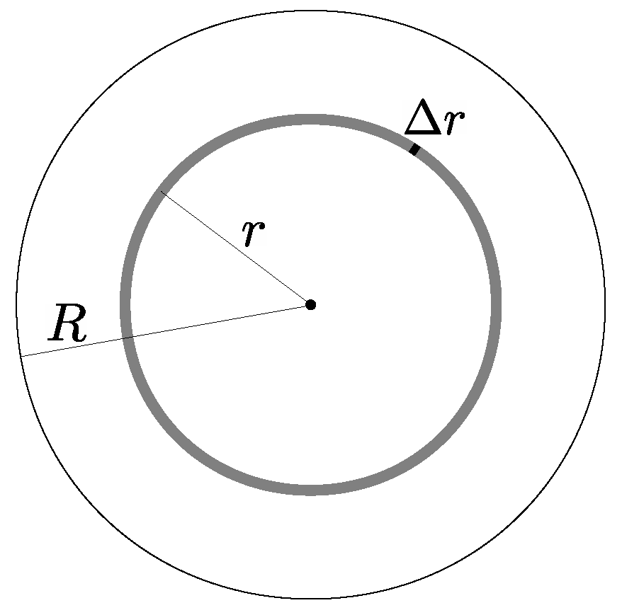
Assume that the area S is divided into n disjoint subsets, , , , and . This is called a partition of the area S [33]. The diameter of a subset is the largest distance between any two points within the subset and diameter of the entire partition is the largest diameter among all . According to Theorem 1 the average load of area S is given by
where and are the average area load and the area’s measure of each partition member, respectively. The sum of Equation (11) can be seen as a Riemann sum [33] and by following the Riemann theory of integration, Equation (11) becomes an integral when (or ). The measure of each subarea tends to zero (), the average load of each subarea becomes the average point load and the corresponding area is written as , in terms of the integral formalism. □
Theorem 3 provides a straightforward interpretation for . If the average point load is constant throughout an area S then it coincides with the average load L of that area. However, in the general case some subareas of S might have different average load of some other subareas, i.e., the average load of the area S changes from point to point. In such cases shows how the average load of S changes from point to point. Note that the average load of a single point is not a measurable magnitude by itself. It must be always integrated over an area in order to provide a meaningful and measurable result.
7. Joint Probability Density Function for a Hop
The rest of this paper focuses on the traffic load in multi-hop networks. This is the most interesting case, compared to receptions load and energy consumption load, since traffic load (a) is directly related to the routing policy; (b) is not affected by the energy consumption model; and (c) apparently depends on the distance from the sink. The following three sections present the newly defined average area and point load in a real case. The adjective “average” will be omitted henceforth, since both the area load and the point load are valid terms only when they are referred to their average values.
Let us assume a simple routing policy, where each node chooses a proper neighbor and forwards all the packets (its own packets along with the packets received by other nodes) to this neighbor. Consequently, the flow of packets towards the sink forms a tree with the sink as the root. Details about how each node selects the particular neighbor are not important here. Let us also assume that each node generates one packet per time unit and all these packets are traveling from node-to-node uncompressed. It has already been mentioned in Section 3 that the number of packets each node transmits is called traffic load of that node.
Consider that a node u chooses the neighbor v as its next hop towards the sink (Figure 4). The euclidean distance between nodes u and v is denoted by h and is referred to as the hop-length of u. The direction of the hop forms an angle with the line that joins the position of u and the sink (the sink direction from u), as depicted in Figure 4. We will refer to this angle as the hop-direction. Consequently, the hop from u to v can be seen as a vector with measure h (hop-length) and direction (hop-direction).
Suppose that the random experiment of Section 3 is performed once and k nodes happen to fall within a fixed area S. Let us write the k nodes as , , …,. Each one of them has a corresponding hop vector , , …,. The average hop of S, for this experiment, is defined as the resultant of these k vectors, divided by k,
The particular direction of can be defined as the angle between the vector itself and the line defined by the geometric center of S (the centroid) and the position of the sink, as depicted in Figure 5.
If we repeat the random experiment many times then follows some joint probability density function (joint-pdf henceforth), denoted by , where and are the measure and the direction of respectively (hop-length and hop-direction of ). Function is the probability density for to be a vector with hop-length and direction . The term “joint” has been used here because the outcome of the experiment gives a combination of two random variables, hop-length and hop-direction. The term “probability density” is due to the fact that both hop-length and hop-direction are continuous random variables.
In an analogous manner as in Section 4, the average hop of the area S is defined as the expected value of or equivalently the expected value of the joint-pdf . Similarly to Section 6.2, if is a nested sequence around the point and then the average hop of becomes the average hop at point and the joint-pdf of becomes the joint-pdf at that point. The average hop of a point will be denoted by , the average hop-length by h and the average hop-direction by . In general, the joint-pdf of a point depends on the position of that point and therefore it can be written as . Without being too mathematically strict, can be seen as the probability (in terms of density) to have a hop with departure point , hop-length h and hop-direction . Since is a probability density function it must satisfy
for every point of the network area . Note that the point is fixed for the integration of Equation (13). The integral is calculated over all possible hops departed from . If the communication range is c then the double integral in Equation (13) can be calculated over the disk that is centered at the point and has radius c, instead of the entire network area.
8. Circular Networks
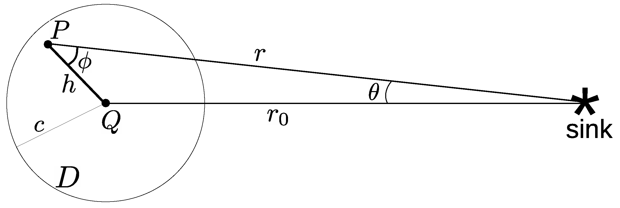
The analysis can be significantly simplified in the case of a circular network. For the rest of this paper it will be assumed that the network covers a disk-shaped area and the sink is positioned at the center of the disk. The network’s shape remains the same after a rotation around the sink. Moreover, all existing routing policies are isotropic, i.e., a rotation of the network does not change any path from each node to the sink. More formally, the output of the routing function (Equation (1)) is the same after a rotation of the network around any point by any arbitrary angle. Recall also that the nodes’ deployment is uniformly random and therefore, nodes’ surface density is constant and unchanged after a rotation. Consequently, a disk-shaped network with the sink at the center has central symmetry with respect to the sink and, consequently, all magnitudes related to the routing will also be centrally symmetric. The interest here is for the traffic load and the joint-pdf at any point . Due to the central symmetry, both magnitudes are independent from the relative direction with respect to the sink and depend only on the distance from the sink. In polar coordinates the position of a point is described as , where r is the distance from the sink (the radius of the point) and the polar angle with respect to some arbitrary axis. For simplicity, the distance between a point and the sink will be henceforth referred to as the radius r of that point, meaning the radius of its polar coordinates. Eventually, in polar coordinates the traffic load can be written as and the joint-pdf as .
Consider a fixed point Q with radius and a disk D with radius c (the communication range) and center the point Q (Figure 6). All points within D have some probability to select the point Q as their next hop. Let the point P be an arbitrary point of the disk D, with polar coordinates . The polar axis for the definition of the polar angle is the direction of Q with respect to the sink (the direction of ). For the hop from P to Q, the distance is the hop-length h and the angle the hop-direction, as presented in Figure 6. The joint probability density function for the pair h, to occur simultaneously is the joint-pdf .
Point Q sees that all points within D have some probability density function to choose it as the next hop. The total probability for Q to be chosen is . If we consider the hop from P to Q as our favorable outcome among all possible hops targeting Q, then the probability for this hop to occur is
Every time the point P chooses the point Q as its next hop all packets of P are transferred to the point Q. The number of the transmitted packets at point P is the traffic load of P. From a traffic load point of view, every time the hop from P to Q occurs, the traffic load of P is transferred to the point Q, i.e., Equation (14) corresponds to the probability for traffic load to be transferred at point Q. Point Q receives the traffic load from all points within D, with a different probability for each point. The total traffic load that point Q receives from the disk D is
where is the total transferred load at point Q.
In polar coordinates the area’s differential is . The magnitudes of h and can be expressed as functions of r and by resolving the triangle of r, and h. If we apply the law of cosines and the law of sines to the aforementioned triangle we can express h and as functions and (the details of these expressions are trivial and omitted). In both integrals of Equation (15) the variable r takes values between and . For each value of r the angle takes values between and as shown in Figure 7. Clearly, is a function of r, i.e., . After the above substitutions, the integral of the nominator of Equation (15) becomes
The internal integral of Equation (16) does not depend on the polar angle and therefore it can be written as . If we repeat the same calculations on the denominator of Equation (15) then it becomes
Equation (17) is the weighed average of in the interval , with weighed function . The weighed mean value theorem for integrals states that for two functions , such that f is continuous and g is integrable in the interval , the following holds true,
where [34]. In the terminology of the weighed mean value theorem for integrals, is the mean value of the function and the weighed function. In the case of Equation (17), the weighed mean value theorem for integrals says that the value of equals the value of at some radius between and . If z denotes the difference between that radius and the then that radius can be written as . Eventually, Equation (17) can be written as
where . Since traffic load is expected to be a decreasing function of r (the closer to sink the higher the load) it can be assumed that for the usual routing mechanisms is satisfied. Note also that Equation (19) is still valid at points close to the periphery. In this case, the integrals of Equation (15) can be calculated over a clipped disk and then, the reasoning until Equation (19) remains the same, except from the integration’s limits which will be clipped accordingly.
Equation (19) hides all the complexity of the random environment behind the variable z. At some distance from the sink a point receives as much load as the load at a longer distance, but no longer than one radio-range. Conclusively, traffic load increases in steps or “hops” and z is the length of these hops. For that reason we will refer to z as load progress. The term “progress” is widely used as a measure for the displacement towards the sink [35,36], especially in geographical routing policies [37]. From Equations (16) and (17) it is clear that the value of z is determined by the combination of the weighed function and the function of load .
9. The Case of Constant Load Progress
This section assumes that load progress z is independent from radius r and has a constant value throughout the network. This is the simplest form of z and, in addition, it makes the estimation of traffic load almost straightforward. Although it is not clear which attributes of the routing policy result in such a simple load progress, it will be assumed that there exists an ideal routing policy that leads to a constant z. In the next section, the results of this section will be compared with the traffic load of some real-world routing policies.
The network is uniform, therefore, the nodes’ surface density (nodes per area unit) is constant and is denoted by . Consider an elementary ring with radius r and infinitesimal width , as shown in Figure 8. The area of the ring is and the number of nodes within this area is . The number of packets that has been transferred to the ring is and the extra packets that have been generated by the ring itself are . Thus, the ring transmits packets in total. The number of the transmitted packets can be computed by the traffic load directly, because the nodes of the ring have the same radius r and therefore the same traffic load . They transmit packets in total. Either calculation must yield the same magnitude, therefore,
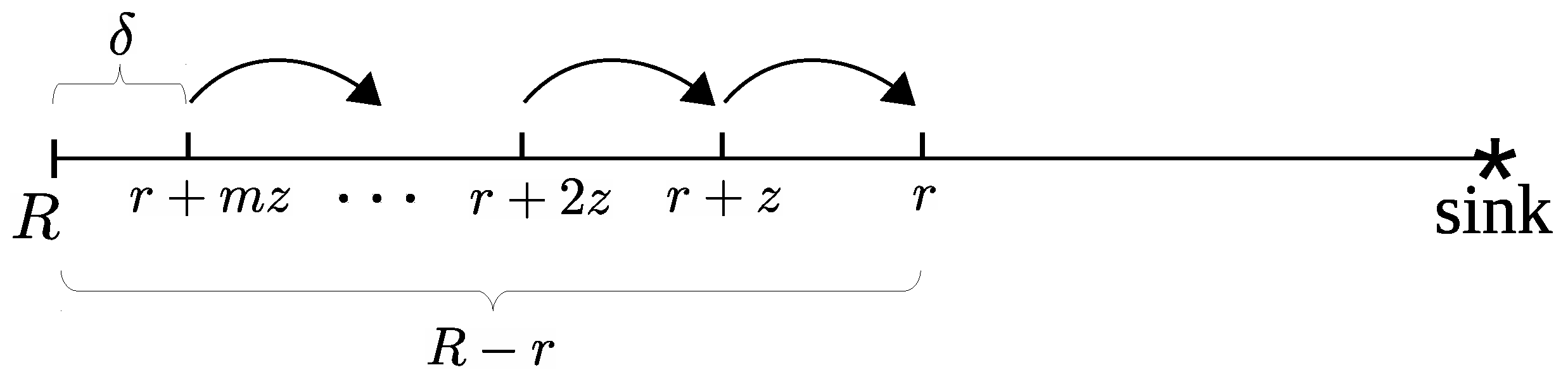
According to Equation (19), load increases in “hops” with length z. The number of packets that have been transferred to the ring, i.e., , is equal to the number of packets that has been received at radius , i.e., , plus the extra packets of the ring at the radius , i.e., . That is
Equation (21) can be applied recursively m times, as Figure 9 shows. The distance from the radius r to the network boundary is and m is the quotient of the euclidean division of by z,
where is the remainder.
The recursion ends because the ring at distance transmits only the packets generated by itself. The addition of the left and right sides of Equation (23) yields
By substituting the value of m from Equation (22) and ignoring (negligible when compared to R), Equation (24) is written as
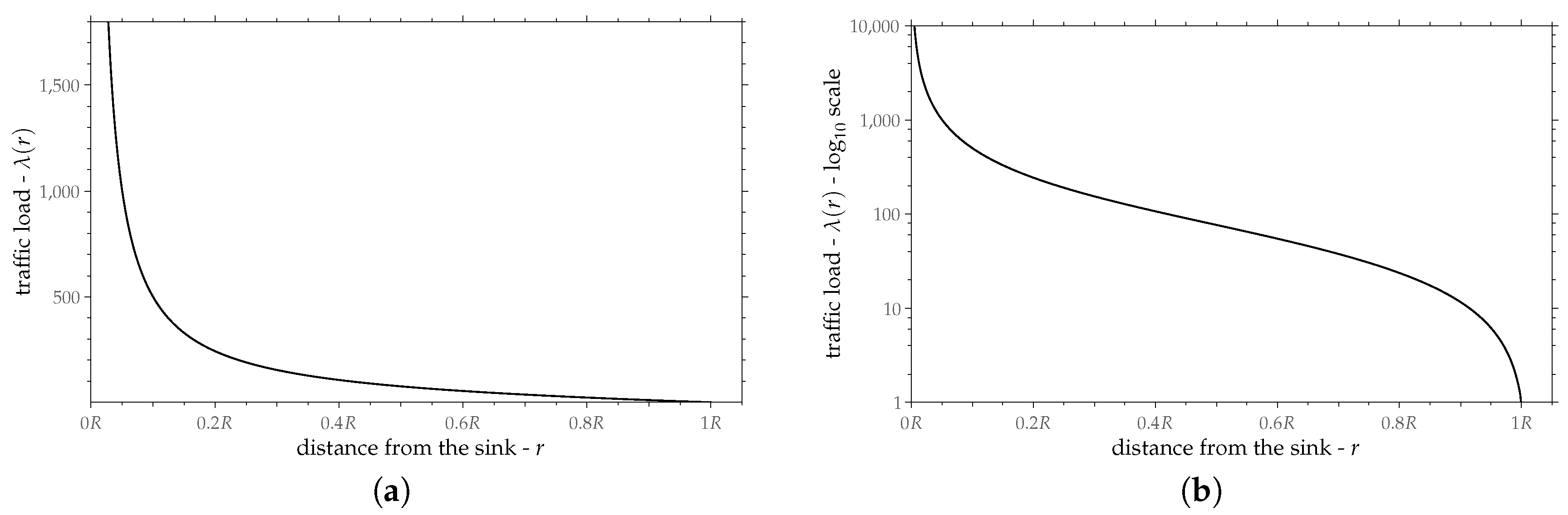
Figure 10 shows a typical graph of Equation (25). Traffic load is a decreasing function of r. It takes the value 1 at the periphery (). This is the expected behavior, since the periphery transmits only its own packets. However, the ideal routing assumes that traffic load goes to infinity for distances too close to the sink and this cannot be true for real-world routings.
10. Results
In Section 9 it was assumed an ideal routing policy that has the same load progress z regardless of the distance from the sink r. However, this is not always true for all routing policies. This section compares the traffic load of some existing (implemented in devices) routing policies with that of the ideal routing.
Simulations are conducted in a custom java program. Each network instance contains 2000 nodes, randomly deployed over a circular area with radius . Nodes’ radio-range is chosen as the of network radius R, in order to have on average 10 neighbors per node [38]. Each node produces one packet, which is delivered to the sink by some routing policy. For each node the number of the transmitted packets equals the traffic load of that node. In order to approximate the traffic load at a point, the radius R is divided into 30 equal intervals (or rings). The average traffic load over the nodes that happen to fall within a ring is the traffic load for that ring and for one network instance, as given by Equation (2). In order to approximate the traffic load’s expected value, 250 networks are constructed (different network instances) and for each ring, the mean value over these networks is computed. This approximates the area’s traffic load L of each ring, as given by Equation (3). Due to the fact that the rings are too narrow, the points within each ring have almost the same traffic load. Therefore, the traffic load of the ring approximates the point traffic load at the middle of the ring (the median point between the interior and exterior ring’s radii). The resulting point’s traffic load (or equivalently the ring’s load) is depicted as a small gray circle in the figures of this section (one circle per ring).
The aim here is to see how well Equation (25) describes the traffic load as a function of the radius r. The only unknown variable in Equation (25) is the load progress z. This can be estimated by the method of least squares, a well-known statistical procedure in regression analysis [39]. The goodness of fit between the resulting curve and the simulated points is evaluated by the Coefficient of Determination (COD) [39]. The value of corresponds to a perfect fit, whereas, values close to zero show no fit at all.
Equation (25) has been compared with the simulated traffic load for eight routing policies. These are:
- (a)
- Minimum Hop Count, also known as Minimum Delay Tree, Breadth First Tree or Shortest (in number of hops) Path Tree. Nodes are aware of their hop number, that is the minimum number of hops from the node to the sink. Each node forwards its packets towards a neighbor with less hop number than the node itself. The resulting tree is the same with that of the Dijkstra’s or Bellman-Ford algorithm, if the edge cost is considered as 1 for all edges.
- (b)
- Shortest Path. The classic Dijkstra or Bellman-Ford algorithm, where edge cost is the euclidean distance between nodes.
- (c)
- Minimum Transmission Energy. The same as (b) the only difference being the edge cost. Here, edge cost is a power of the distance between the two edge’s nodes, with the exponent usually defined between 2 and 4 [40]. In that way, edge cost becomes proportional to the required energy for transmission, hence the name. The exponent that has been used for this comparison is 2. Larger exponents give similar (and in some cases even better) results, but they are not included here.
- (d)
- Sink Betweenness Routing [41]. Sink betweenness is a centrality measure attributed to a node, which shows how likely is it for that node to become a hot-spot. Each node shares its packets among the neighbors that are closer (in number of hops) to the sink than the node itself. Nodes that are more likely to be hot-spots (higher sink betweenness) receive less packets than the others. Packets are delivered to the sink in a multi-path manner, since there is no tree formation in this policy.
- (e)
- -Shortest Path [42]. Same as (b) with the difference being that the edge cost is multiplied by a factor after each hop, starting from the sink to the tree leaves. That way edges close to the sink become more important than the distant ones. The value of has been used for this comparison. Different values for a give similar results as those presented here.
- (f)
- Minimum Spanning Tree. The classic tree of minimum total edge cost (Prim’s or Kruskal’s algorithm). Edge cost is the euclidean distance between nodes.
- (g)
- Greedy Geographical Forwarding. The most common of the position-based routing policies [43]. Nodes forward their packets to the particular neighbor that minimizes the distance from the sink, i.e., the one that is closer to the sink. No other infrastructure is needed, apart from the knowledge of the distance from the sink.
- (h)
- Minimum Residual Energy [40]. Same as (b) but with edge cost the inverse of the neighbor’s residual energy. Edge cost changes after a transmission, therefore, the tree does not remain constant. Is is considered here that the initial energy is the same for all nodes. The residual energy after the first nodal loss is taken into account and the resulting tree is considered to be a representative one for this routing policy.
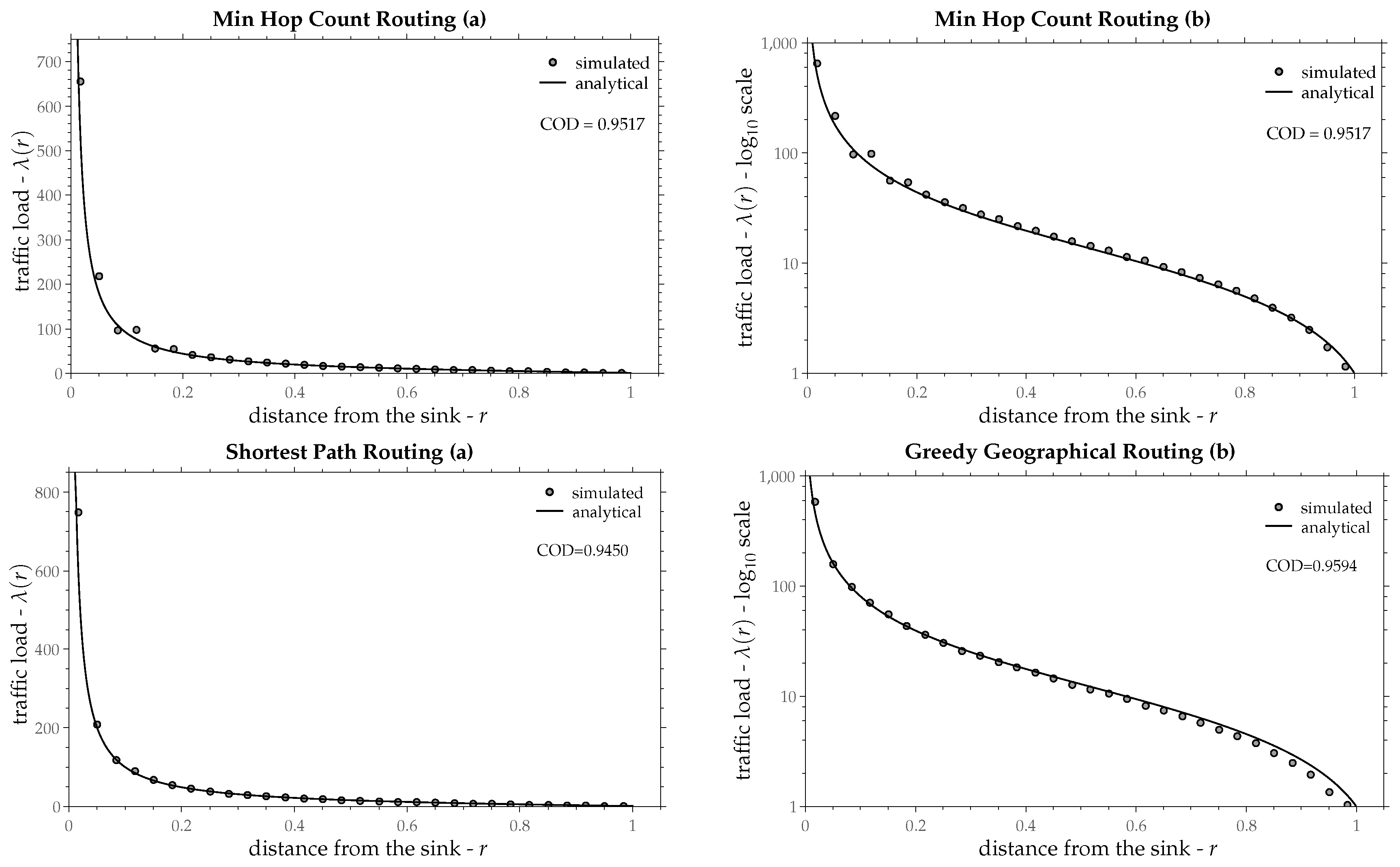
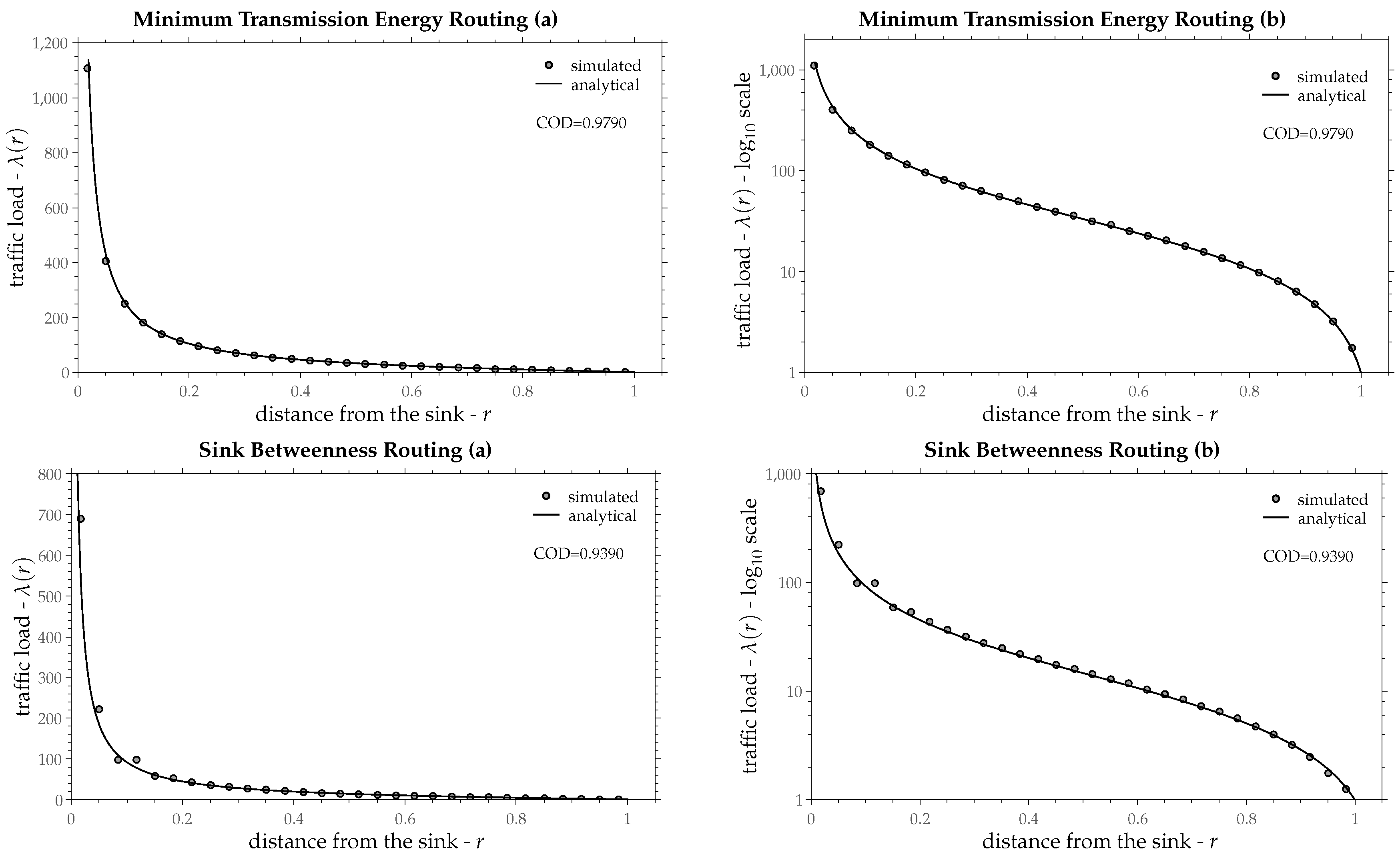
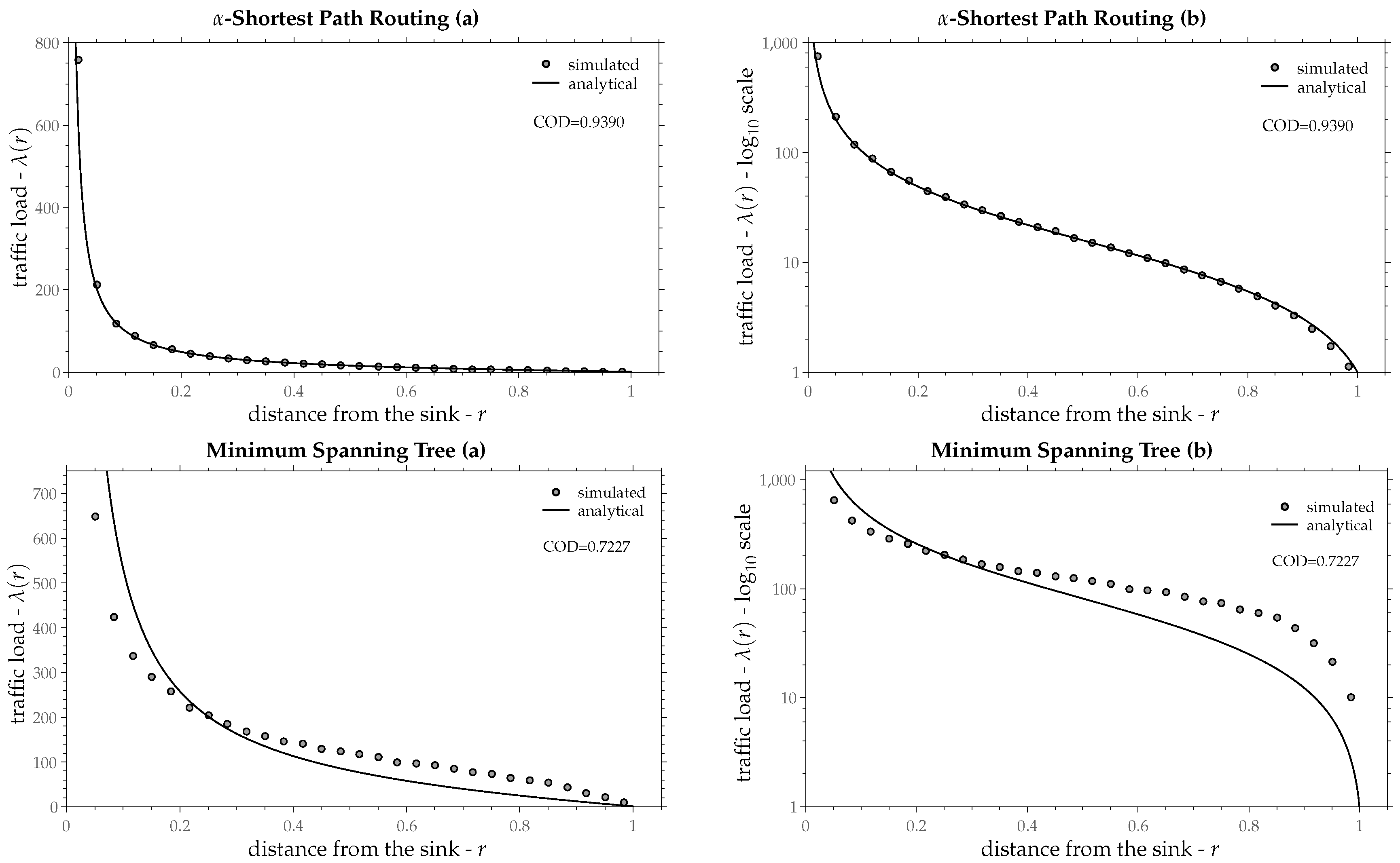
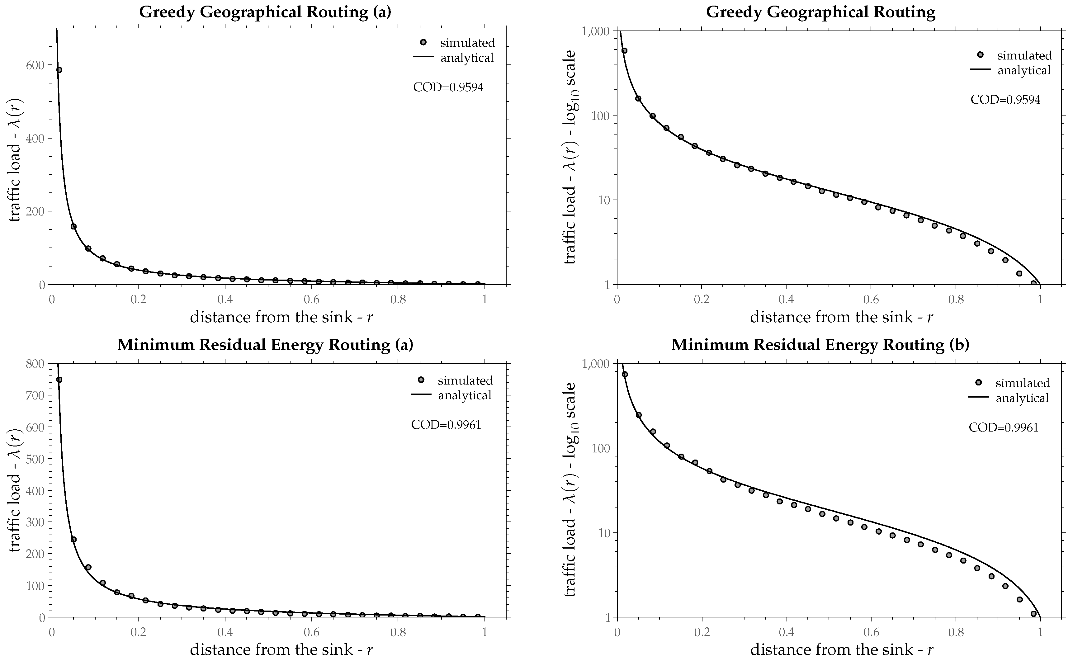
Figure 11, Figure 12, Figure 13 and Figure 14 present the graph of Equation (25) as a continuous line and the simulated traffic load as small gray circles. Table 1 shows the estimated values of load progress z as a percentage of the radio-range along with the confidence interval 95% and the coefficient of determination for the aforementioned routing policies. In most routing policies Equation (25) fits upon the simulated points fairly well and in some of them almost perfectly, except for the Minimum Spanning Tree, in which traffic load is increased in a quite different way as Equation (25) suggests. Recall that the derivation of Equation (25) was based on a constant load progress z throughout the network (independently from radius r). The assumption of a constant z seems to be valid in most routing policies, especially at points that are not too close to the sink.
11. Conclusions
This paper provides a consistent definition of the term “average load” for both an area and a point within a random wireless sensor network. The average area load is defined as the expected value of the average of those nodes that happen to fall within the area. If an area is reduced (or contracted) to a single point, then the average area load converges to the average point load. It has been proved here that the average area load is the integral of the average point load over the area, divided by the area’s measure. The average point load is not a measurable magnitude on its own. It requires to be always integrated over an area and divided by the area’s measure in order to provide the average load of that area.
These definitions, introduced in this paper, have been applied in the case of traffic load in multi-hop networks. Especially for circular networks, traffic load increases in steps, similar to the packet’s hops. The assumption that these steps are independent from radius (distance from the sink) leads to a simple analytical expression for the traffic load. The analytical expression attains to describe the traffic load of many routing policies fairly well and in some cases very well. The assumption that traffic load increases in constant steps appears to be valid or almost valid in many existing routing policies.
In conclusion, the study of load as presented in this paper gives insight into the particulars of an attribute that affects—among other attributes—network lifetime and eventually the nature of the supported applications. Given that the emerging 5G mobile technology will give a new perspective to wireless sensor applications for assistive environments like personal health-care, smart home and smart city applications, etc., the outcomes of this paper will help evaluate future applications in the considered network environment.
Author Contributions
Both authors have equally contributed in this paper.
Funding
This research received no external funding.
Acknowledgments
This work was supported in part by project “A Pilot Wireless Sensor Networks System for Synchronized Monitoring of Climate and Soil Parameters in Olive Groves,” (MIS 5007309) which is partially funded by European and National Greek Funds (ESPA) under the Regional Operational Programme “Ionian Islands 2014-2020”.
Conflicts of Interest
The authors declare no conflict of interest.
Abbreviations
The following abbreviations are used in this manuscript:
| Variables | |
| N | Total number of nodes |
| c | Communication range or radio-range |
| Routing function | |
| Area of the entire network | |
| S | An area within the network |
| D | A disk-shaped area with radius c |
| A | Measure of an area (e.g., in m) |
| R | The radius of a circular network |
| ℓ | Load of an individual node for a single execution of the random experiment |
| Average area load for a single execution of the random experiment | |
| L | Average area load (or simply area load) |
| Average point load (or simply point load) | |
| Vector representation of a hop | |
| h | Measure of , or hop-length |
| Direction of , or hop-direction | |
| The vector of the average hop for an area and for a single execution of the random experiment | |
| The measure of | |
| Joint probability density function of , or joint-pdf for an area | |
| Joint probability density function at point | |
| r | Distance from the sink in polar coordinates |
| Polar angle in polar coordinates | |
| T | The traffic load that is transferred at a point from its neighborhood |
| z | Load progress |
| Surface density of nodes (nodes per unit area) | |
| COD | Coefficient of Determination |
| joint-pdf | joint probability density function |
References
- Akyildiz, I.F.; Su, W.; Sankarasubramaniam, Y.; Cayirci, E. Wireless sensor networks: A survey. Comput. Netw. 2002, 38, 393–422. [Google Scholar] [CrossRef]
- Xu, L.; Collier, R.; O’Hare, G.M.P. A Survey of Clustering Techniques in WSNs and Consideration of the Challenges of Applying Such to 5G IoT Scenarios. IEEE Internet Things J. 2017, 4, 1229–1249. [Google Scholar] [CrossRef]
- Akpakwu, G.A.; Silva, B.J.; Hancke, G.P.; Abu-Mahfouz, A.M. A Survey on 5G Networks for the Internet of Things: Communication Technologies and Challenges. IEEE Access 2018, 6, 3619–3647. [Google Scholar] [CrossRef]
- Woo, M.W.; Lee, J.; Park, K. A reliable IoT system for Personal Healthcare Devices. Future Gener. Comput. Syst. 2018, 78, 626–640. [Google Scholar] [CrossRef]
- Qi, J.; Yang, P.; Min, G.; Amft, O.; Dong, F.; Xu, L. Advanced internet of things for personalised healthcare systems: A survey. Pervasive Mob. Comput. 2017, 41, 132–149. [Google Scholar] [CrossRef]
- Skouby, K.E.; Lynggaard, P. Smart home and smart city solutions enabled by 5G, IoT, AAI and CoT services. In Proceedings of the 2014 International Conference on Contemporary Computing and Informatics (IC3I), Mysore, India, 27–29 November 2014; pp. 874–878. [Google Scholar]
- Erdelj, M.; Król, M.; Natalizio, E. Wireless Sensor Networks and Multi-UAV systems for natural disaster management. Comput. Netw. 2017, 124, 72–86. [Google Scholar] [CrossRef]
- Yick, J.; Mukherjee, B.; Ghosal, D. Wireless sensor network survey. Comput. Netw. 2008, 52, 2292–2330. [Google Scholar] [CrossRef]
- Anastasi, G.; Conti, M.; Di Francesco, M.; Passarella, A. Energy conservation in wireless sensor networks: A survey. Ad Hoc Netw. 2009, 7, 537–568. [Google Scholar] [CrossRef] [Green Version]
- Rault, T.; Bouabdallah, A.; Challal, Y. Energy efficiency in wireless sensor networks: A top-down survey. Comput. Netw. 2014, 67, 104–122. [Google Scholar] [CrossRef] [Green Version]
- Li, H.; Pandit, V.; Agrawal, D.P. Gaussian distributed deployment of relay nodes for wireless Visual Sensor Networks. In Proceedings of the Global Communications Conference (GLOBECOM), Anaheim, CA, USA, 3–7 December 2012; pp. 5374–5379. [Google Scholar]
- Yang, Y.; Fonoage, M.I.; Cardei, M. Improving network lifetime with mobile wireless sensor networks. Comput. Commun. 2010, 33, 409–419. [Google Scholar] [CrossRef]
- Bhagyalakshmi, L.; Suman, S.K.; Murugan, K. Corona based clustering with mixed routing and data aggregation to avoid energy hole problem in wireless sensor network. In Proceedings of the 2012 Fourth International Conference on Advanced Computing (ICoAC), Chennai, India, 13–15 December 2012; pp. 1–8. [Google Scholar]
- Liu, A.; Liu, Z.; Nurudeen, M.; Jin, X.; Chen, Z. An elaborate chronological and spatial analysis of energy hole for wireless sensor networks. Comput. Stand. Interfaces 2013, 35, 132–149. [Google Scholar] [CrossRef]
- Asharioun, H.; Asadollahi, H.; Wan, T.C.; Gharaei, N. A Survey on Analytical Modeling and Mitigation Techniques for the Energy Hole Problem in Corona-Based Wireless Sensor Network. Wirel. Pers. Commun. 2015, 81, 161–187. [Google Scholar] [CrossRef]
- Wu, X.; Chen, G.; Das, S.K. Avoiding Energy Holes in Wireless Sensor Networks with Nonuniform Node Distribution. IEEE Trans. Parallel Distrib. Syst. 2008, 19, 710–720. [Google Scholar] [CrossRef] [Green Version]
- Chen, Q.; Kanhere, S.S.; Hassan, M. Analysis of per-node traffic load in multi-hop wireless sensor networks. IEEE Trans. Wirel. Commun. 2009, 8, 958–967. [Google Scholar] [CrossRef]
- Li, J.; Mohapatra, P. Analytical modeling and mitigation techniques for the energy hole problem in sensor networks. Pervasive Mob. Comput. 2007, 3, 233–254. [Google Scholar] [CrossRef]
- Demertzis, A.; Oikonomou, K. Analysis of Concise “Average Load” Definitions in Uniformly Random Deployed Wireless Sensor Networks. In Proceedings of the 11th PErvasive Technologies Related to Assistive Environments Conference, Corfu, Greece, 26–29 June 2018; ACM: New York, NY, USA, 2018; pp. 17–22. [Google Scholar]
- Luo, J.; Hubaux, J.P. Joint mobility and routing for lifetime elongation in wireless sensor networks. In Proceedings of the IEEE 24th Annual Joint Conference of the IEEE Computer and Communications Societies, Miami, FL, USA, 13–17 March 2005; Volume 3, pp. 1735–1746. [Google Scholar]
- Wang, Q.; Zhang, T. Traffic load distribution in large-scale and dense wireless sensor networks. In Proceedings of the 5th International ICST Conference on Wireless Internet, Singapore, 1–3 March 2010; pp. 1–8. [Google Scholar]
- Ren, J.; Zhang, Y.; Zhang, K.; Liu, A.; Chen, J.; Shen, X.S. Lifetime and energy hole evolution analysis in data-gathering wireless sensor networks. IEEE Trans. Ind. Inf. 2016, 12, 788–800. [Google Scholar] [CrossRef]
- Ammari, H.M.; Das, S.K. Promoting heterogeneity, mobility, and energy-aware voronoi diagram in wireless sensor networks. IEEE Trans. Parallel Distrib. Syst. 2008, 19, 995–1008. [Google Scholar] [CrossRef]
- Haenggi, M.; Andrews, J.; Baccelli, F.; Dousse, O.; Franceschetti, M. Stochastic geometry and random graphs for the analysis and design of wireless networks. IEEE J. Sel. Areas Commun. 2009, 27, 1029–1046. [Google Scholar] [CrossRef] [Green Version]
- Haenggi, M. Stochastic Geometry for Wireless Networks; Cambridge University Press: Cambridge, UK, 2013; p. 284. [Google Scholar]
- Shi, G.; Liao, M.; Ma, M.; Shu, Y. Exploiting sink movement for energy-efficient load-balancing in wireless sensor networks. In Proceedings of the 1st ACM International Workshop on Foundations of Wireless Ad Hoc and Sensor Networking and Computing, Hong Kong, China, 26 May 2008; pp. 39–44. [Google Scholar]
- Chatterjee, P.; Das, N. A distributed algorithm for load-balanced routing in multihop wireless sensor networks. In Distributed Computing and Networking; Springer: Berlin/Heidelberg, Germany, 2008; pp. 332–338. [Google Scholar]
- Shan, M.; Chen, G.; Luo, D.; Zhu, X.; Wu, X. Building maximum lifetime shortest path data aggregation trees in wireless sensor networks. ACM Trans. Sens. Netw. 2014, 11, 11. [Google Scholar] [CrossRef]
- Liu, A.; Jin, X.; Cui, G.; Chen, Z. Deployment guidelines for achieving maximum lifetime and avoiding energy holes in sensor network. Inf. Sci. 2013, 230, 197–226. [Google Scholar] [CrossRef]
- Broder, A. Generating random spanning trees. In Proceedings of the 30th Annual Symposium on Foundations of Computer Science, Research Triangle Park, NC, USA, 30 October–1 November 1989; pp. 442–447. [Google Scholar]
- Papoulis, A.; Pillai, S.U. Probability, Random Variables, and Stochastic Processes, 4th ed.; Tata McGraw-Hill Education: New York, NY, USA, 2002; p. 850. [Google Scholar]
- Knight, K. Mathematical Statistics; Chapman & Hall/CRC Texts in Statistical Science; Taylor & Francis: Thames, UK, 1999. [Google Scholar]
- Rudin, W. Principles of Mathematical Analysis; McGraw-Hill: New York, NY, USA, 1964; Volume 3. [Google Scholar]
- Polezzi, M. On the weighted mean value theorem for integrals. Int. J. Math. Educ. Sci. Technol. 2006, 37, 868–870. [Google Scholar] [CrossRef]
- Takagi, H.; Kleinrock, L. Optimal transmission ranges for randomly distributed packet radio terminals. IEEE Trans. Commun. 1984, 32, 246–257. [Google Scholar] [CrossRef]
- Lian, J.; Chen, L.; Naik, K.; Otzu, T.; Agnew, G. Modelling and enhancing the data capacity of wireless sensor networks. IEEE Monogr. Sens. Netw. Oper. 2004, 2, 91–138. [Google Scholar]
- Giordano, S.; Stojmenovic, I.; Blazevic, L. Position based routing algorithms for ad hoc networks: A taxonomy. In Ad hoc Wireless Networking; Springer: Boston, MA, USA, 2004; pp. 103–136. [Google Scholar]
- Demertzis, A.; Oikonomou, K. Avoiding energy holes in wireless sensor networks with non-uniform energy distribution. In Proceedings of the 5th International Conference on Information, Intelligence, Systems and Applications, Chania, Greece, 7–9 July 2014; pp. 138–143. [Google Scholar]
- Draper, N.R.; Smith, H. Applied Regression Analysis; John Wiley & Sons: Hoboken, NJ, USA, 2014; Volume 326. [Google Scholar]
- Chang, J.H.; Tassiulas, L. Energy conserving routing in wireless ad-hoc networks. In Proceedings of the IEEE INFOCOM 2000 Conference on Computer Communications, Nineteenth Annual Joint Conference of the IEEE Computer and Communications Societies, Tel Aviv, Israel, 26–30 March 2000; Volume 1, pp. 22–31. [Google Scholar]
- Ramos, H.S.; Frery, A.C.; Boukerche, A.; Oliveira, E.M.R.; Loureiro, A.A.F. Topology-related metrics and applications for the design and operation of wireless sensor networks. ACM Trans. Sens. Netw. 2014, 10, 53. [Google Scholar] [CrossRef]
- Bechkit, W.; Koudil, M.; Challal, Y.; Bouabdallah, A.; Souici, B.; Benatchba, K. A new weighted shortest path tree for convergecast traffic routing in WSN. In Proceedings of the 2012 IEEE Symposium on Computers and Communications (ISCC), Cappadocia, Turkey, 1–4 July 2012; pp. 000187–000192. [Google Scholar]
- Stojmenovic, I.; Lin, X. Loop-free hybrid single-path/flooding routing algorithms with guaranteed delivery for wireless networks. IEEE Trans. Parallel Distrib. Syst. 2001, 12, 1023–1032. [Google Scholar] [CrossRef] [Green Version]
Figure 1.
Addition of average area loads.

Figure 2.
A nested sequence of areas around .

Figure 3.
Decomposition of into and .

Figure 4.
Hop from u to v as a vector .

Figure 5.
Average hop of an area S for a network instance (a single execution of the random experiment).
Figure 5.
Average hop of an area S for a network instance (a single execution of the random experiment).

Figure 6.
A hop from P to Q.

Figure 7.
The integration of Equation (16). For each r between and corresponds an angle , which is a function of r.
Figure 7.
The integration of Equation (16). For each r between and corresponds an angle , which is a function of r.

Figure 8.
A ring with infinitesimal width .

Figure 9.
Derivation of Equation (22).
Figure 9.
Derivation of Equation (22).

Figure 10.
Traffic load versus distance from the sink as given by Equation (25), (a) normal plot, (b) semi-log (log-linear) plot.
Figure 10.
Traffic load versus distance from the sink as given by Equation (25), (a) normal plot, (b) semi-log (log-linear) plot.

Figure 11.
Comparison between Equation (25) and the simulated traffic load as a function of the distance from the sink for two routing schemes, Min Hop Count and Shortest Path. (a) normal (linear) plot, (b) semi-log plot (log-linear).
Figure 11.
Comparison between Equation (25) and the simulated traffic load as a function of the distance from the sink for two routing schemes, Min Hop Count and Shortest Path. (a) normal (linear) plot, (b) semi-log plot (log-linear).

Figure 12.
Comparison between Equation (25) and the simulated traffic load as a function of the distance from the sink, for two routing schemes, Minimum Transmission Energy and Sink Betweenness. (a) normal (linear) plot, (b) semi-log plot (log-linear).
Figure 12.
Comparison between Equation (25) and the simulated traffic load as a function of the distance from the sink, for two routing schemes, Minimum Transmission Energy and Sink Betweenness. (a) normal (linear) plot, (b) semi-log plot (log-linear).

Figure 13.
Comparison between Equation (25) and the simulated traffic load as a function of the distance from the sink, for two routing schemes, -Shortest Path and Minimum Spanning Tree. (a) normal (linear) plot, (b) semi-log plot (log-linear).
Figure 13.
Comparison between Equation (25) and the simulated traffic load as a function of the distance from the sink, for two routing schemes, -Shortest Path and Minimum Spanning Tree. (a) normal (linear) plot, (b) semi-log plot (log-linear).

Figure 14.
Comparison between Equation (25) and the simulated traffic load as a function of the distance from the sink, for two routing schemes, Greedy Geographical and Minimum Residual Energy. (a) normal (linear) plot, (b) semi-log plot (log-linear).
Figure 14.
Comparison between Equation (25) and the simulated traffic load as a function of the distance from the sink, for two routing schemes, Greedy Geographical and Minimum Residual Energy. (a) normal (linear) plot, (b) semi-log plot (log-linear).


Table 1.
Load progress z and Coefficient of Determination (COD) for the compared routing policies.
| Policy | Load Progress z along with the Confidence Interval 95% as a Portion of the Range c | Coefficient of Determination |
|---|---|---|
| Minimum Hop Count | 0.829 ± 0.065 | 0.9517 |
| Shortest Path | 0.741 ± 0.056 | 0.9450 |
| Minimum Transmission Energy | 0.335 ± 0.007 | 0.9790 |
| Sink Betweenness | 0.808 ± 0.069 | 0.9390 |
| -Shortest Path | 0.739 ± 0.059 | 0.9390 |
| Minimum Spanning Tree | 0.133 ± 0.005 | 0.7227 |
| Greedy Geographical | 0.932 ± 0.076 | 0.9594 |
| Minimum Residual Energy | 0.623 ± 0.011 | 0.9961 |
© 2018 by the authors. Licensee MDPI, Basel, Switzerland. This article is an open access article distributed under the terms and conditions of the Creative Commons Attribution (CC BY) license (http://creativecommons.org/licenses/by/4.0/).
Share and Cite
MDPI and ACS Style
Demertzis, A.; Oikonomou, K. Average Load Definition in Random Wireless Sensor Networks: The Traffic Load Case. Technologies 2018, 6, 112. https://doi.org/10.3390/technologies6040112
AMA Style
Demertzis A, Oikonomou K. Average Load Definition in Random Wireless Sensor Networks: The Traffic Load Case. Technologies. 2018; 6(4):112. https://doi.org/10.3390/technologies6040112
Chicago/Turabian StyleDemertzis, Apostolos, and Konstantinos Oikonomou. 2018. "Average Load Definition in Random Wireless Sensor Networks: The Traffic Load Case" Technologies 6, no. 4: 112. https://doi.org/10.3390/technologies6040112
Note that from the first issue of 2016, this journal uses article numbers instead of page numbers. See further details here.