Stability Analysis of Plankton–Fish Dynamics with Cannibalism Effect and Proportionate Harvesting on Fish

Abstract

Plankton occupy a vital place in the marine ecosystem due to their essential role. However small or microscopic, their absence can bring the entire life process to a standstill. In this work, we have proposed a prey–predator ecological model consisting of phytoplankton, zooplankton, and fish, incorporating the cannibalistic nature of zooplankton harvesting the fish population. Due to differences in their feeding habits, zooplankton are divided into two sub-classes: herbivorous and carnivorous. The dynamic behavior of the model is examined for each of the possible steady states. The stability criteria of the model have been analyzed from both local and global perspectives. Hopf bifurcation analysis has been accomplished with the growth rate of carnivorous zooplankton using cannibalism as a bifurcation parameter. To characterize the optimal control, we have used Pontryagin’s maximum principle. Subsequently, the optimal system has been derived and solved numerically using an iterative method with Runge–Kutta fourth-order scheme. Finally, to facilitate the interpretation of our mathematical results, we have proceeded to investigate it using numerical simulations.

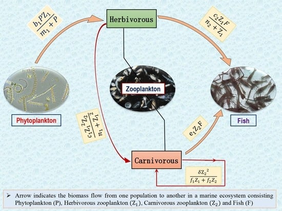
1. Introduction

Life consists of a series of implication and decomposition processes fueled by the energy from highly energetic chemical bonds present in organic matter. In marine ecology, organic matter is mainly generated by microscopic, unicellular plants, which are part of the plankton [1,2,3]. Plankton is a fundamental pillar of many food web structures and controls many ecosystems [4,5,6,7]. Zooplankton are essential in marine food webs, not only because of their abundance and high diversity but also for their vital trophic ecosystem functions—especially in the aquatic food web [2,8]. They are the main grazers of phytoplankton and the main prey for many fish and other higher trophic levels [9,10,11,12]. The balance of the aquatic food web is bound to be disturbed if the exploitation rate of marine fish rises unchecked, as they are the main plankton balancers in the marine ecosystem [9,13,14]. Recently, we have observed that the ecological system is often deeply altered by human parasitical activities, such as the absorption of biological resources and harvest of the population, which are commonly studied in fishery fields [13,14,15,16]. Thus, there is a rapidly growing interest in modeling and analyzing biological systems with harvesting.

Phytoplankton are the ’primary producers’, meaning they take inorganic materials such as nitrogen and carbon and convert them into biomass through photosynthesis [2,3]. The main limiting factors for phytoplankton growth are nutrient availability and light; on account of this, phytoplankton populations are restricted to the upper layers of lakes and oceans [5,6,9,10]. Zooplankton are tiny animals in the water bodies. Their main food source is phytoplankton, microscopic plants that provide most of the matter and energy in marine systems [11,13,14]. Zooplanktons are considered the most important link between planktonic primary producers and large carnivorous, among them fish species (Figure 1) subject to human exploitation [17,18]. Thus, the research on phytoplankton, zooplankton, and fish dynamics is essential for our society due to their universal existence and importance.

Historically, Malthus [19] first proposed the population growth model in population biology, and Verhulst [20] improved upon it to make it more applicable to the real world. Lotka and Volterra both provided an independent explanation of how the cycle in biological populations started [21,22]. In the study of the predator–prey model, the most important thing to look at is the functional response, which is the rate at which predator populations consume their prey. Different types of functional responses lead to different kinds of dynamics between the populations that are interacting with each other [23,24,25,26]. To study the dynamics of the predator–prey models, Holling developed three different types of functional response, namely Type I, Type II, and Type III [27,28,29]. Holling type I–III functional responses are clear examples of monotonic functions in the positive quadrant. However, it has been seen and tested that there is also a non-monotonic function and that when the concentration of nutrients is high, it may slow down the growth rate of a specific organism. Andrews came up with a new form of the response function, which is called the Monod–Haldane function [30]. It is also called the Holling type IV functional response, and it has been used by several researchers to solve the problem of high concentration [31,32,33,34]. The important effect of the type II functional response is seen when numbers eaten per predator are re-expressed as a proportion of the living prey population alive. The functional response of herbivores is not as well known as those of carnivores. In actual application, it has to be determined whether there is a type II or III response function because the difference occurs at low density of prey [35,36,37].

Cannibalism among members of the same species is one of the major concerns in the context of a prey–predator relationship [38,39,40,41]. Cannibalism is the act of one individual of a species consuming all or part of another individual of the same species as food. To consume the same species or show cannibalistic behavior is a common ecological interaction in the animal kingdom and has been recorded for more than 1500 species [42]. Several studies have demonstrated that cannibalism has a variety of positive and negative repercussions on the dynamics and longevity of populations [43,44,45,46]. These effects, among others, include a potential for alternative stable states [47,48] and chaotic dynamics [49]. Due to the act of cannibalism, there is a clear gain to the cannibalistic predator, but fully cannibalistic predators are unable to sustain the population [50]. However, many cannibalistic models ignore the energy that cannibals gain from cannibalism and are, essentially, "infanticide" models [43,45,49]. Theoretical research suggests that the cannibal’s energy drain may have a major bearing on both the longevity of the population and the lives of its members [44]. In this context, in the present study, we incorporated the effect of cannibalism on the dynamics of a prey–predator system governed by phytoplankton, zooplankton, and fish species.

The harvesting of a species is another key issue that arises within a prey–predator system. Harvesting is the process of catching, taking, or removing (animals), especially for food [51,52]. It is vital for social management and the protection of resources, both from an economic and ecological point of view [14,53]. For the ecosystem to grow and stay healthy in the 21st century, it is important to make good use of biotic resources. The over-availability of prey or predator species, or both prey and predator species, can exploit a system [15,16,54]. It is necessary to harvest the species at a certain level in order to prevent the system from being exploited. Harvesting at the right time and in the right way maximizes grain yield and minimizes grain losses and quality deterioration [54,55]. Many people throughout the whole world are dependent on the harvesting of fish because it is a favorite food source for human beings. Therefore, harvesting is necessary for the economic development of a country. However, over or continuous harvesting of a particular species may cause the extinction of that species. Hence, a suitable optimal control strategy is necessary for the conservation of species [14,15,40,54].

The remaining parts of this paper are organized as follows: Next section deals with the required assumption and model formulation with an ecological description of associated model parameters and variables. The positivity and boundedness of all solutions of the proposed model are tested in Section 3. The next section provides the existence of different equilibrium points and their stability, as well as the global stability around the interior equilibrium point. In Section 5, the Hopf bifurcation point is calculated with respect to some important parameters. Section 6 deals with the optimal control theory, which is used to determine the optimal harvesting rate, followed by Section 7, in which some numerical simulations are presented. The paper is concluded by Section 8 with a detailed discussion of the ecological prospect of each equilibrium point and remarks on harvesting for economic improvement.

2. Formulation of the Model

The main goal of this section is to have a proper mathematical understanding to quantify the effect of cannibalism and harvesting on plankton–fish interaction predator–prey system. Before moving on to model formulation, we have described the model parameters and variables in their ecological context to facilitate understanding the mathematical model.

2.1. Model Variables and Parameters

During the process of developing the model (1), in the following

Table 1. Parameters introduced in the model with their ecological/biological description.

Parameter	Ecological/Biological Description
P	Total phytoplankton population.
$Z_1$	Total herbivorous zooplankton population.
$Z_2$	Total carnivorous zooplankton population.
F	Total fish population.
r	Intrinsic growth rate of phytoplankton.
K	Environmental carrying capacity of phytoplankton.
$b_1$	Capture rate.
$m_1$	(Holling Type II) Half saturation constant.
${\alpha }_1$	Conversion rate of herbivorous zooplankton.
$c_1$	Capture rate.
$n_1$	(Holling Type III) Half saturation constant.
$d_1$	Death rate of herbivorous zooplankton.
${\beta }_1$	Conversion rate of carnivorous zooplankton.
$e_1$	Efficiency of predation.
$c_2$	Capture rate.
$n_2$	(Holling Type II) Half saturation constant.
$d_2$	Death rate of carnivorous zooplankton.
$\xi$	Growth rate of carnivorous zooplankton due to cannibalism.
$\delta$	Rate of cannibalism.
${\gamma }_1$	Efficiency of conversion of herbivorous zooplankton to fish population.
${\gamma }_2$	Efficiency of conversion of carnivorous zooplankton to fish population.
$d_3$	Death rate of fish.
q	Catchability coefficient.
E	Effort applied to harvest the fish species.

, the variables and parameters have been taken into consideration, and their respective descriptions have been provided.

2.2. Assumptions and Model Formulation

To study the impact of cannibalism and harvesting on the plankton–fish interaction predator–prey system, a three-species predator–prey interaction model has been considered among phytoplankton (P), zooplankton (Z), and fish (F). Before giving our mathematical model, we make the following assumptions:

(i)

It is assumed in our proposed model that zooplankton species are divided into two subclasses as $\left(a\right)$ herbivorous zooplankton $\left(Z_1\right)$ and $\left(b\right)$ carnivorous zooplankton $\left(Z_2\right)$, because the zooplankton community at any trophic level is represented by herbivorous and carnivorous according to their distinctive food habits.

(ii)

In the absence of zooplankton, the phytoplankton population growth obeys the logistic law with intrinsic growth rate r and the carrying capacity of the environment K.

(iii)

It is assumed that only herbivorous zooplankton consumes phytoplankton by following the Holling type II response function with consumption rate $b_1$ and a half saturation constant $m_1$. This response reflects the predator’s ability to handle and process prey at a maximum rate. Many planktonic predators exhibit type II functional responses, including zooplankton such as rotifers and small crustaceans. These organisms can actively search for and capture prey, and their consumption rate typically increases with prey density until a point of satiation is reached.

(iv)

The fish species consumes both herbivorous zooplankton as well as carnivorous zooplankton. The consumption of herbivorous zooplankton by fish is modeled as Holling type II functional response with half saturation constant ($n_2$). On the other hand, the functional response for predation to carnivorous zooplankton by fish species is assumed to be taken as the Holling type I response function. In the type I response, the predator’s feeding rate increases linearly with the prey density until it reaches a saturation point. However, the type II response shows an initial rapid increase in the predator’s feeding rate, which eventually levels off as prey density continues to increase. Predators (fish) typically respond to a decreasing density of prey by removing a constant (type I functional response) or increasing (type II functional response) fraction of the remaining prey. Switching permits a predator, when given a choice of alternate prey, to alter its functional response to prey in low abundance in order to feed more effectively on prey in greater abundance. Under certain conditions, this behavior can stabilize fluctuations in populations of prey by providing a refuge from predation for rare prey.

(v)

The consumption of carnivorous zooplankton to herbivorous zooplankton is modeled as Holling type III response function with consumption rate $c_1$ and half-saturation constant $n_1$. The representation of this type of functional response is more appropriate for situations in which the predation rate per capita prey tends to become smaller as the density of prey decreases, which may often occur if there are refuges for prey or there is another predator for the same prey. A type III functional response is characterized by a sigmoidal curve, where the predator’s consumption rate is initially slow at low prey densities, then accelerates rapidly as prey density increases, and finally plateaus or slows down again at high prey densities. Type III functional responses are commonly observed in predators that exhibit prey-switching behavior or have complex foraging strategies. In plankton ecosystems, some larger zooplankton species may display type III functional responses.

(vi)

Cannibalism is a biological phenomenon used by some species due to limited food availability. Here cannibalism is considered on carnivorous zooplankton species depending on both the herbivorous and carnivorous zooplankton. Thus, the food available for carnivorous zooplankton is $(f_1{Z}_1+f_2{Z}_2)$ with cannibalism rate $\delta$. Due to the act of cannibalism, there is a clear gain for the cannibalistic predator. This gain results in an increase in reproduction in carnivorous zooplankton with reproduction rate $\xi$. This, in turn, leads to a gain in the carnivorous zooplankton population which is expressed by the term $\xi Z_2$.

Keeping the above assumptions in mind, our proposed model is formulated by the following system of differential equations, and the outline of the whole scenario of the model (1) is presented with the help of a schematic diagram (Figure 2):

Figure 2. Schematic representation of the plankton–fish interaction system (1).

Figure 2. Schematic representation of the plankton–fish interaction system (1).

$$\begin{array}{c}\hfill \left.\begin{array}{c}\frac{dP}{dt}=rP(1-\frac{P}{K})-\frac{b_{1}P{Z}_1}{m_1+P}\hfill \\ \\ \frac{d{Z}_1}{dt}=\frac{{\alpha }_1{b}_{1}P{Z}_1}{m_1+P}-\frac{c_1{Z}_1^2{Z}_2}{n_1+Z_1^2}-\frac{c_2{Z}_{1}F}{n_2+Z_1}-d_1{Z}_1\hfill \\ \\ \frac{d{Z}_2}{dt}=\frac{{\beta }_1{c}_1{Z}_1^2{Z}_2}{n_1+Z_1^2}-e_1{Z}_{2}F-\frac{\delta Z_2^2}{f_1{Z}_1+f_2{Z}_2}+\xi Z_2-d_2{Z}_2\hfill \\ \\ \frac{dF}{dt}=\frac{{\gamma }_1{c}_2{Z}_{1}F}{n_2+Z_1}+{\gamma }_2{e}_1{Z}_{2}F-d_{3}F-qEF\hfill \end{array}\right\}\end{array}$$

(1)

with initial conditions $P\left(0\right)\ge 0$, $Z_1\left(0\right)\ge 0$, $Z_2\left(0\right)\ge 0$, and $F\left(0\right)\ge 0$. The description of model parameters and variables with their ecological meaning are given in Table 1.

3. Positivity and Boundedness of Solutions

In this section, we discuss the positivity and boundedness of all solutions of our proposed model (1). That a biological model’s solutions are both positive and bounded is important because it shows that the system is meaningful from an ecological point of view. Any solutions that start from a point inside the first quadrant always stay in that quadrant. As a result, the test of positivity and boundedness of a biological model system (1) is required, and we are eager to demonstrate it.

3.1. Positivity

Theorem 1. 

The solution $\left(P\left(t\right),Z_1\left(t\right),Z_2\left(t\right),F\left(t\right)\right)$ of system (1) is positive for all $t\ge 0$ if $P\left(0\right)>0$, $Z_1\left(0\right)>0$, $Z_2\left(0\right)>0$, and $F\left(0\right)>0$.

Proof. 

To show the positivity of all system solutions (1), we have considered the following differential equations of that system.

$$\begin{array}{ccc}\frac{dP}{dt}\hfill & =& rP(1-\frac{P}{K})-\frac{b_{1}P{Z}_1}{m_1+P}\hfill \end{array}$$

(2)

$$\begin{array}{ccc}\frac{d{Z}_1}{dt}\hfill & =& \frac{{\alpha }_1{b}_{1}P{Z}_1}{m_1+P}-\frac{c_1{Z}_1^2{Z}_2}{n_1+Z_1^2}-\frac{c_2{Z}_{1}F}{n_2+Z_1}-d_1{Z}_1\hfill \end{array}$$

(3)

$$\begin{array}{ccc}\frac{d{Z}_2}{dt}\hfill & =& \frac{{\beta }_1{c}_1{Z}_1^2{Z}_2}{n_1+Z_1^2}-e_1{Z}_{2}F-d_2{Z}_2+\xi Z_2-\frac{\delta Z_2^2}{f_1{Z}_1+f_2{Z}_2}\hfill \end{array}$$

(4)

$$\begin{array}{ccc}\frac{dF}{dt}\hfill & =& \frac{{\gamma }_1{c}_2{Z}_{1}F}{n_2+Z_1}+{\gamma }_2{e}_1{Z}_{2}F-d_{3}F-qEF\hfill \end{array}$$

(5)

Now, from the Equation (2), we see that the right-hand side of (2) is a continuous function of the dependent variable, so after integrating and using the initial condition $P\left(0\right)>0$, we obtain

$$\begin{array}{c}\hfill P\left(t\right)=P\left(0\right)exp\left[{\int }_0^t\left\{r(1-\frac{P\left(s\right)}{K})-\frac{b_1{Z}_1\left(s\right)}{m_1+P\left(s\right)}\right\}ds\right]\end{array}$$

(6)

Similarly, we integrate the Equations (3)–(5) and using the initial conditions $Z_1\left(0\right)>0$, $Z_1\left(0\right)>0$, and $F\left(0\right)>0$, respectively, which give the following:

$$\begin{array}{c}\hfill Z_1\left(t\right)=Z_1\left(0\right)exp\left[{\int }_0^t\left\{\frac{{\alpha }_1{b}_{1}P\left(s\right)}{m_1+P\left(s\right)}-\frac{c_1{Z}_1\left(s\right)Z_2\left(s\right)}{n_1+Z_1^2\left(s\right)}-\frac{c_{2}F\left(s\right)}{n_2+Z_1\left(s\right)-d_1}\right\}ds\right]\end{array}$$

(7)

$$\begin{array}{c}\hfill Z_2\left(t\right)=Z_2\left(0\right)exp\left[{\int }_0^t\left\{\frac{{\beta }_1{c}_1{Z}_1^2\left(s\right)}{n_1+Z_1^2\left(s\right)}-e_{1}F\left(s\right)-d_2+\xi -\frac{\delta Z_2\left(s\right)}{f_1{Z}_1\left(s\right)-f_2{Z}_2\left(s\right)}\right\}ds\right]\end{array}$$

(8)

and

$$\begin{array}{c}\hfill F\left(t\right)=F\left(0\right)exp\left[{\int }_0^t\left\{\frac{{\gamma }_1{c}_2{Z}_1\left(s\right)}{n_2+Z_1\left(s\right)}-{\gamma }_2{e}_1{Z}_2\left(s\right)-d_3-qE\right\}ds\right]\end{array}$$

(9)

Because the part in the right-hand side of (6), (7), (8), and (9) are positive for all positive initial conditions, hence all solutions of the system (1) that start from ${\mathbb{R}}_{+}^4$ also remain in ${\mathbb{R}}_{+}^4=\{P\left(0\right)>0,Z_1\left(0\right)>0,Z_2\left(0\right)>0$, $F\left(0\right)>0\}$ for all $t\ge 0$.

This completes the proof of the positivity of solutions of the system (1). □

3.2. Boundedness

Theorem 2. 

All the solutions of the system (1) that satisfy the initial condition $\left(P\right(0)\ge 0$, $Z_1\left(0\right)\ge 0$, $Z_2\left(0\right)\ge 0$, $F\left(0\right)\ge 0)$ are uniformly bounded in the region $\Omega =\left\{(P,Z_1,Z_2,F)\in {\mathbb{R}}_{+}^4:0<P\le K,0<{\alpha }_{1}P+Z_1+\frac{1}{{\beta }_1}{Z}_2+\frac{1}{{\gamma }_1}F\le \frac{D}{\eta }\right\}$.

Proof. 

From the first equation of system (1) we have

$$\begin{array}{ccc}\hfill \frac{dP}{dt}& =& rP(1-\frac{P}{K})-\frac{b_{1}P{Z}_1}{m_1+P}\hfill \\ & \le & rP(1-\frac{P}{K})\hfill \end{array}$$

Using the standard comparison theorem [56], we obtain

$$P\left(t\right)\le K\mathrm{for}\mathrm{all}t\ge 0$$

Now, to prove the boundedness of all solutions of our proposed model (1), we consider the following function

$$\begin{array}{c}\hfill W\left(t\right)={\alpha }_{1}P\left(t\right)+Z_1\left(t\right)+\frac{1}{{\beta }_1}{Z}_2\left(t\right)+\frac{1}{{\gamma }_1}F\left(t\right)\end{array}$$

(10)

Calculating the time derivative of W, we obtain

$$\begin{array}{ccc}\hfill \frac{dW\left(t\right)}{dt}& =& {\alpha }_1\frac{dP}{dt}+\frac{d{Z}_1}{dt}+\frac{1}{{\beta }_1}\frac{d{Z}_2}{dt}+\frac{1}{{\gamma }_1}\frac{dF}{dt}\hfill \\ & =& {\alpha }_{1}rP(1-\frac{P}{K})-d_1{Z}_1-\frac{e_1}{{\beta }_1}{Z}_{2}F-\frac{d_2}{{\beta }_1}{Z}_2+\frac{\xi }{{\beta }_1}{Z}_2-\frac{\delta }{{\beta }_1}\frac{Z_2^2}{f_1{Z}_1+f_2{Z}_2}\hfill \\ & & -\frac{{\gamma }_2{e}_1}{{\gamma }_1}{Z}_{2}F-\frac{d_3}{{\gamma }_1}F-\frac{qE}{{\gamma }_1}F\hfill \end{array}$$

Without loss of generality, we assume that the number of individuals lost for cannibalism is always greater than the newly individuals directly produced from cannibalism [50]. It is also assumed that the conversion of carnivorous zooplankton to fish due to predation is dominated by the loss of carnivorous zooplankton to avoid population explosion. Therefore, we have

$$\begin{array}{ccc}\hfill \frac{dW\left(t\right)}{dt}& \le & {\alpha }_{1}rP(1-\frac{P}{K})-d_1{Z}_1-\frac{d_2}{{\beta }_1}{Z}_2-\frac{d_3}{{\gamma }_1}F-\frac{qE}{{\gamma }_1}F\hfill \end{array}$$

Let us choose a $\eta (>0)$ such that

$$\frac{dW\left(t\right)}{dt}+\eta W\le \frac{{\alpha }_{1}K{(r+\eta )}^2}{4r}-(d_1-\eta )Z_1-\frac{1}{{\beta }_1}(d_2-\eta )Z_2-\frac{1}{{\gamma }_1}(d_3+qE-\eta )F$$

Now, we define $\eta \le min\{d_1,d_2,d_3\}$ and take $D=\frac{{\alpha }_{1}K{(r+\eta )}^2}{4r}$. Then we have

$$\begin{array}{ccc}& & \frac{dW\left(t\right)}{dt}+\eta W\left(t\right)\le D\hfill \end{array}$$

Therefore,

$$0<W\left(t\right)\le \frac{D}{\eta }+\left(W\left(0\right)-\frac{D}{\eta }\right)e^{-\eta t}$$

As $t\to \infty$, $W\left(t\right)\to \frac{D}{\eta }$

$$i.e.,W\left(t\right)\le \frac{D}{\eta },\mathrm{since}\underset{t\to \infty }{sup}W\left(t\right)=\frac{D}{\eta }$$

Hence all solutions of the system (1) are uniformly bounded.

This result implies that none of the interacting species grow abruptly over long periods of time. Because of limited resources, the number/abundance of each species is bounded. □

4. Equilibria and Stability Analysis

In this section, different equilibrium points are determined. In addition, the stability of the proposed system (1) is analyzed around these equilibrium points.

4.1. Equilibrium Points

The equilibrium points of the respective system (1) are necessary to calculate for the study of the stability analysis of the system (1). Now, different possible equilibrium points of the system (1) are given below:

(i)

The trivial equilibrium $E_0(0,0,0,0)$ always exists.

(ii)

The zooplankton and fish free axial equilibrium $E_1(K,0,0,0)$ always exists on the boundary of the first octant.

(iii)

The carnivorous zooplankton and fish free planar equilibrium $E_2(\tilde{P},\widetilde{Z_1},0,0)$, where

$\tilde{P}=\frac{d_1{m}_1}{{\alpha }_1{b}_1-d_1}$ and $\widetilde{Z_1}=\frac{{\alpha }_{1}r{m}_1\{K{\alpha }_1{b}_1-d_1(K+m_1)\}}{K{({\alpha }_1{b}_1-d_1)}^2}.$

Now, the planar equilibrium $E_2(\tilde{P},\widetilde{Z_1},0,0)$ exists if $d_1<min\{{\alpha }_1{b}_1,{\alpha }_1{b}_1\left(\frac{K}{K+m_1}\right)\}$, which implies $d_1<{\alpha }_1{b}_1\left(\frac{K}{K+m_1}\right)$. Therefore, the carnivorous zooplankton and fish free equilibrium exists if the natural mortality rate of the herbivorous zooplankton is less than a threshold value, which is determined by other biological parameters.

(iv)

The fish free equilibrium $E_4(\overline{P},\overline{Z_1},\overline{Z_2},0)$, where $\overline{P}=\frac{m_1\{c_1\overline{Z_1}\overline{Z_2}+d_1{(n_1+\overline{Z_1})}^2\}}{({\alpha }_1{b}_1-d_1)(n_1+{\overline{Z_1}}^2)-c_1\overline{Z_1}\overline{Z_2}}$, $\overline{Z_1}=\frac{r}{b_1}(1-\frac{\overline{P}}{K})(m_1+\overline{P})$ and $\overline{Z_2}=\frac{f_1\overline{Z_1}\{(d_2-\xi )(n_1+{\overline{Z_1}}^2)-{\beta }_1{c}_1{\overline{Z_1}}^2\}}{f_2{\beta }_1{c}_1{\overline{Z_1}}^2-(n_1+{\overline{Z_1}}^2)\{(d_2-\xi )f_2-\delta \}}$.

Now, the equilibrium $E_4(\overline{P},\overline{Z_1},\overline{Z_2},0)$ exists if $\overline{P}<K$, $\xi <d_2$, $b_1>\frac{1}{{\alpha }_1}\left(\frac{c_1\overline{Z_2}}{\overline{Z_1}}+d_1\right)$ and $n_1>\left(\frac{{\beta }_1{c}_1}{d_2-\xi }-1\right)$. Therefore, the fish free equilibrium exists if the consumption rate of herbivorous zooplankton to phytoplankton and the half-saturation constant is greater than their respective threshold value, which is determined by other biological parameters of the system (1).

(v)

The carnivorous zooplankton free equilibrium $E_5(\widehat{P},\widehat{Z_1},0,\widehat{F})$, where

$\widehat{P}=\frac{-(m_1-K)+\sqrt{{(m_1-K)}^2-4(\frac{b_1\widehat{Z_1}}{r}-m_1)}}{2}$, $\widehat{Z_1}=\frac{n_2(d_3+qE)}{{\gamma }_1{c}_2-(d_3+qE)}$, and $\widehat{F}=\frac{n_2+\widehat{Z_1}}{c_2}(\frac{{\alpha }_1{b}_1\widehat{P}}{m_1+\widehat{P}}-d_1)$

Now, the equilibrium $E_5(\widehat{P},\widehat{Z_1},0,\widehat{F})$ exists if $r>\frac{b_1\widehat{Z_1}}{m_1}$ and ${\gamma }_1>\frac{1}{c_2}(d_3+qE)$. Therefore, the carnivorous zooplankton free equilibrium exists if the intrinsic growth rate of phytoplankton and conversion efficiency of herbivorous zooplankton to fish population through predation is greater than their respective threshold value, which is determined by other biological parameters.

(vi)

The interior equilibrium $E^{*}(P^{*},Z_1^{*},Z_2^{*},F^{*})$, where $P^{*}=\frac{m_{1}H}{{\alpha }_1{b}_1-H}$, $Z_1^{*}=\frac{r}{b_1}(1-\frac{P^{*}}{K})(m_1+P^{*})$, $Z_2^{*}=\frac{1}{{\gamma }_2{e}_1}\left\{(d_3+qE)-\frac{{\gamma }_1{c}_2{Z}_1^{*}}{n_2+Z_1^{*}}\right\}$ and $F^{*}=\frac{1}{e_1}\{(\xi -d_2)+\frac{{\beta }_1{c}_1{Z}_1^{*2}}{n_1+Z_1^{*2}}-\frac{\delta Z_2^{*}}{f_1{Z}_1^{*}+f_2{Z}_2^{*}}\}$. It is noted that, $H=\frac{c_1{Z}_1^{*}{Z}_2^{*}}{m_1+Z_1^{*2}}+\frac{c_2{F}^{*}}{n_2+Z_1^{*}}+d_1$. Now, the interior equilibrium $E^{*}(P^{*},Z_1^{*},Z_2^{*},F^{*})$ exists if $K>P^{*}$, ${\alpha }_{>}\frac{H}{b_1}$, $d_3>\frac{{\gamma }_1{c}_2{Z}_1^{*}}{n_2+Z_1^{*}}-qE$ and $\xi >d_2+\frac{\delta Z_2^{*}}{f_1{Z}_1^{*}+f_2{Z}_2^{*}}-\frac{{\beta }_1{c}_1{Z}_1^{*2}}{n_1+Z_1^{*2}}$. Therefore, the interior equilibrium $E^{*}$ exists if the conversion to the newly juvenile carnivorous zooplankton is directly produced through cannibalism and the natural mortality rate of fish are greater than their respective threshold values. These threshold values are determined by other biological parameters associated with the system (1). Now, from the existence condition of the interior equilibrium $E^{*}$ it is noted that the critical threshold of $\xi$ is obtained and is denoted by ${\xi }^{*}=d_2+\frac{\delta Z_2^{*}}{f_1{Z}_1^{*}+f_2{Z}_2^{*}}-\frac{{\beta }_1{c}_1{Z}_1^{*2}}{n_1+Z_1^{*2}}$

Remark 1. 

From the third equation of system (1), it is seen that the carnivorous zooplankton ($Z_2$) cannibalize on their juveniles at a rate δ and this cannibalism has a conversion factor ξ. Therefore, if there is no predation occurring, then there is a possibility for carnivorous zooplankton to grow individually, such as phytoplankton, due to cannibalism. That means herbivorous zooplankton and fish free equilibrium $E_3(P,0,Z_2,0)$ may occur. However, a biological restriction on the efficiency of cannibalism is the number of juveniles lost to cannibalism is always greater than the new juveniles directly produced from cannibalism, and fully cannibalistic predators are unable to sustain the population [50]. Thus, from the third equation of the system (1), it is observed that the rate of change in carnivorous zooplankton ($Z_2$) with respect to time is negative. There is no predation occurring because the gain in the zooplankton population is dominated by the loss of juveniles due to cannibalism. Hence, the occurrence of herbivorous zooplankton and fish free equilibrium $E_3(P,0,Z_2,0)$ is nearly impossible in a biological context.

4.2. Stability Analysis

In this section, we analyze the local stability of the system (1) in the neighborhood of the different equilibrium points.

Theorem 3. 

The trivial equilibrium point $E_0(0,0,0,0)$ is always unstable.

Proof. 

The corresponding Jacobian matrix at $E_0$ is given by

$$\begin{array}{c}\hfill {\left[J\right]}_{E_0}=\left(\begin{array}{cccc}r& 0& 0& 0\\ 0& -d_1& 0& 0\\ 0& 0& -d_2+\xi & 0\\ 0& 0& 0& -(d_3+qE)\end{array}\right)\end{array}$$

The corresponding eigenvalues are r, $-d_1$, $-(d_2-\xi )$, and $-(d_3+qE)$. As one eigenvalue is strictly positive, another eigenvalue will also be positive if $d_2<\xi$. Therefore, the trivial equilibrium is always unstable. □

Theorem 4. 

The zooplankton and fish free equilibrium $E_1(K,0,0,0)$ is locally asymptotically stable if $d_2>\xi$ and $d_1>\frac{{\alpha }_1{b}_{1}K}{m_1+K}$.

Proof. 

The corresponding Jacobian matrix at $E_1$ is given by

$$\begin{array}{c}\hfill {\left[J\right]}_{E_1}=\left(\begin{array}{cccc}-r& -\frac{b_{1}K}{m_1+K}& 0& 0\\ 0& \frac{{\alpha }_1{b}_{1}K}{m_1+K}-d_1& 0& 0\\ 0& 0& -d_2+\xi & 0\\ 0& 0& 0& -(d_3+qE)\end{array}\right)\end{array}$$

The eigenvalues of ${\left[J\right]}_{E_1}$ are $-r$, $\frac{{\alpha }_1{b}_{1}K}{m_1+K}-d_1$, $-d_2+\xi$, and $-(d_3+qE)$. Hence, $E_1$ is locally asymptotically stable if (i) $d_2>\xi$ and (ii) $d_1>\frac{{\alpha }_1{b}_{1}K}{m_1+K}$ hold. $E_1$ loses its stability when either of the conditions (i) or (ii) fails. Therefore, the zooplankton and fish free equilibrium $E_1$ is locally asymptotically stable if the mortality rate of the herbivorous zooplankton and the carnivorous zooplankton is greater than a threshold value, which is determined by other parameters. □

Theorem 5. 

The carnivorous zooplankton and fish free equilibrium $E_2(\tilde{P},\widetilde{Z_1},0,0)$ is locally asymptotically stable if $r<\frac{K{b}_1{m}_1\widetilde{Z_1}}{{(m_1+\tilde{P})}^2(K-2\tilde{P})}$, $d_1>\frac{{\alpha }_1{b}_1\tilde{P}}{(m_1+\tilde{P})}$ and $\xi <d_2-\frac{{\beta }_1{c}_1{\tilde{Z}}_1^2}{n_1+{\widetilde{Z_1}}^2}$.

Proof. 

The corresponding Jacobian matrix at $E_2$ is given by

$$\begin{array}{c}\hfill {\left[J\right]}_{E_2}=\left(\begin{array}{cccc}{A}_1& -A_2& 0& 0\\ A_3& A_4& -A_5& -A_6\\ 0& 0& A_7& 0\\ 0& 0& 0& A_8\end{array}\right)\end{array}$$

where $A_1=r(1-\frac{2\tilde{P}}{K})-\frac{b_1{m}_1\widetilde{Z_1}}{{(m_1+\tilde{P})}^2}$, $A_2=\frac{b_1\tilde{P}}{(m_1+\tilde{P})}$, $A_3=\frac{{\alpha }_1{b}_1{m}_1\widetilde{Z_1}}{{(m_1+\tilde{P})}^2}$, $A_4=\frac{{\alpha }_1{b}_1\tilde{P}}{(m_1+\tilde{P})}-d_1$, $A_5=\frac{c_1{\widetilde{Z_1}}^2}{n_1+{\widetilde{Z_1}}^2}$, $A_6=\frac{c_2\widetilde{Z_1}}{n_2+\widetilde{Z_1}}$, $A_7=\frac{{\beta }_1{c}_1{\widetilde{Z_1}}^2}{n_1+{\widetilde{Z_1}}^2}+\xi -d_2$, $A_8=-(d_3+qE)$.

The eigenvalues of ${\left[J\right]}_{E_2}$ are $r(1-\frac{2\tilde{P}}{K})-\frac{b_1{m}_1\widetilde{Z_1}}{{(m_1+\tilde{P})}^2}$, $\frac{{\alpha }_1{b}_1\tilde{P}}{(m_1+\tilde{P})}-d_1$, $\frac{{\beta }_1{c}_1{\widetilde{Z_1}}^2}{n_1+{\widetilde{Z_1}}^2}+\xi -d_2$ and $-(d_3+qE)$ Hence, $E_2$ is locally asymptotically stable if (i) $r<\frac{K{b}_1{m}_1\widetilde{Z_1}}{{(m_1+\tilde{P})}^2(K-2\tilde{P})}$, (ii) $d_1>\frac{{\alpha }_1{b}_1\tilde{P}}{(m_1+\tilde{P})}$ and (iii) $\xi <d_2-\frac{{\beta }_1{c}_1{\tilde{Z}}_1^2}{n_1+{\widetilde{Z_1}}^2}$ hold. $E_2$ loses its stability when any of the conditions (i), (ii), or (iii) fails. Therefore, the carnivorous zooplankton and fish free equilibrium $E_2$ are locally asymptotically stable if the mortality rate of the herbivorous zooplankton is greater than a threshold value, and the intrinsic growth rate of phytoplankton and the conversion to the newly juvenile carnivorous zooplankton directly produced from cannibalism are less than their respective threshold values. These threshold values are obtained from the other parameters of the system (1). It is noted that the corresponding threshold values of r and $\xi$ are $\frac{K{b}_1{m}_1\widetilde{Z_1}}{{(m_1+\tilde{P})}^2(K-2\tilde{P})}$ and $d_2-\frac{{\beta }_1{c}_1{\tilde{Z}}_1^2}{n_1+{\widetilde{Z_1}}^2}$, respectively. □

Theorem 6. 

The fish free equilibrium $E_4(\overline{P},\overline{Z_1},\overline{Z_2},0)$ is locally asymptotically stable if $A_1>0$, $C_1>0$, $D_1>0$ and $A_1{B}_1{C}_1>C_1^2+A_1^2{D}_1$.

Proof. 

The corresponding Jacobian matrix at $E_4$ is given by

$$\begin{array}{c}\hfill {\left[J\right]}_{E_4}=\left(\begin{array}{cccc}{Q}_1& Q_2& 0& 0\\ Q_3& Q_4& Q_5& Q_6\\ 0& Q_7& Q_8& Q_9\\ 0& 0& 0& Q_{10}\end{array}\right)\end{array}$$

Now, the corresponding characteristic equation at $E_4$ of the above Jacobian matrix is

$$\begin{array}{c}\hfill {\lambda }^4+A_1{\lambda }^3+B_1{\lambda }^2+C_1\lambda +D_1=0\end{array}$$

where the algebraic expression of $A_1$, $B_1$, $C_1$, $D_1$ and all other associated expression are provided in Appendix A.

Thus, according to the Routh–Hurwitz criterion, the above characteristic equation has negative eigenvalues or eigenvalues with negative real parts if $A_1>0$, $C_1>0$, $D_1>0$ and $A_1{B}_1{C}_1>C_1^2+A_1^2{D}_1$. Therefore, the fish free equilibrium $E_4(\overline{P},\overline{Z_1},\overline{Z_2},0)$ is locally asymptotically stable if $A_1>0$, $C_1>0$, $D_1>0$ and $A_1{B}_1{C}_1>C_1^2+A_1^2{D}_1$. □

Theorem 7. 

The carnivorous zooplankton free equilibrium $E_5(\widehat{P},\widehat{Z_1},0,\widehat{F})$ is locally asymptotically stable if $A_2>0$, $C_2>0$, $D_2>0$ and $A_2{B}_2{C}_2>C_2^2+A_2^2{D}_2$.

Proof. 

The corresponding Jacobian matrix at $E_5$ is given by

$$\begin{array}{c}\hfill {\left[J\right]}_{E_5}=\left(\begin{array}{cccc}{M}_1& M_2& 0& 0\\ M_3& M_4& M_5& M_6\\ 0& 0& M_7& 0\\ 0& M_8& M_9& M_{10}\end{array}\right)\end{array}$$

Then, the corresponding characteristic equation at $E_5$ of the above Jacobian matrix is

$$\begin{array}{c}\hfill {\lambda }^4+A_2{\lambda }^3+B_2{\lambda }^2+C_2\lambda +D_2=0\end{array}$$

where the algebraic expression of $A_2$, $B_2$, $C_2$, $D_2$ and all other associated expression are provided in Appendix A.

Thus, according to Routh–Hurwitz criterion the above characteristic equation has negative eigenvalues or eigenvalues with negative real parts if $A_2>0$, $C_2>0$, $D_2>0$ and $A_2{B}_2{C}_2>C_2^2+A_2^2{D}_2$ which imply the carnivorous zooplankton free equilibrium $E_5(\widehat{P},\widehat{Z_1},0,\widehat{F})$ is locally asymptotically stable if $A_2>0$, $C_2>0$, $D_2>0$ and $A_2{B}_2{C}_2>C_2^2+A_2^2{D}_2$. □

Theorem 8. 

The interior equilibrium $E^{*}(P^{*},Z_1^{*},Z_2^{*},F^{*})$ is locally asymptotically stable if $A^{*}>0$, $C^{*}>0$, $D^{*}>0$ and $A^{*}{B}^{*}{C}^{*}>C^{*}{}^2+A^{*}{}^2{D}^{*}$.

Proof. 

The corresponding Jacobian matrix at the interior equilibrium point $E^{*}$ is given by

$$\begin{array}{c}\hfill {\left[J\right]}_{E^{*}}=\left(\begin{array}{cccc}{N}_1& N_2& 0& 0\\ N_3& N_4& N_5& N_6\\ 0& N_7& N_8& N_9\\ 0& N_{10}& N_{11}& N_{12}\end{array}\right)\end{array}$$

Now, the characteristic equation at $E^{*}$ of the above Jacobian matrix is

$$\begin{array}{c}\hfill {\lambda }^4+A^{*}{\lambda }^3+B^{*}{\lambda }^2+C^{*}\lambda +D^{*}=0\end{array}$$

(11)

where the algebraic expression of $A^{*}$, $B^{*}$, $C^{*}$, $D^{*}$ and all other associated expression are provided in Appendix A.

Thus, according to Routh–Hurwitz criterion the above characteristic equation has negative eigenvalues or eigenvalues with negative real parts if $A^{*}>0$, $C^{*}>0$, $D^{*}>0$ and $A^{*}{B}^{*}{C}^{*}>C^{*}{}^2+A^{*}{}^2{D}^{*}$. Therefore, the interior equilibrium $E^{*}(P^{*},Z_1^{*},Z_2^{*},F^{*})$ is locally asymptotically stable if $A^{*}>0$, $C^{*}>0$, $D^{*}>0$ and $A^{*}{B}^{*}{C}^{*}>C^{*}{}^2+A^{*}{}^2{D}^{*}$. □

The expressions for the components of $E^{*}$ cannot be obtained explicitly; hence, the explicit parametric restrictions for the stability of $E^{*}$ cannot be obtained. We use numerical examples to explain the stability of interior equilibrium. For this purpose, we choose the parameter values $r=0.5$, $K=30.0$, $b_1=0.05$, $m_1=2.0$, ${\alpha }_1=0.03$, $c_1=0.5$, $n_1=4.0$, $c_2=0.0002$, $n_2=4.0$, $d_1=0.0001$, ${\beta }_1=0.05$, $e_1=0.1$, $d_2=0.00001$, $\xi =0.01$, $\delta =0.001$, $f_1=1.0$, $f_2=3.0$, ${\gamma }_1=0.3$, ${\gamma }_2=0.6$, $d_3=0.001$, $q=0.1$, $E=0.01$. For this choice of parameter values, we obtain the unique interior equilibrium point $E^{*}=(25.01,0.33,0.03,0.027)$ and (11) becomes

$$\begin{array}{c}\hfill {\lambda }^4+6.3804{\lambda }^3+21.3.16{\lambda }^2+40.2474\lambda +24.7218=0.\end{array}$$

Here $A^{*}$, $C^{*}$ and $D^{*}$ are positive and $A^{*}{B}^{*}{C}^{*}(=5473.22)>\{C^{*}{}^2+A^{*}{}^2{D}^{*}\}$ (=2626.11) and the eigenvalues are $-1.2877\pm 2.6425i$, $-2.7734$ and $-1.3016$. Thus by Routh–Hurwitz criteria, $E^{*}$ is locally asymptotically stable.

4.3. Global Stability

In this section, global stability has been discussed by choosing a suitable Lyapunov function of the system (1) around the interior equilibrium $E^{*}(P^{*},Z_1^{*},Z_2^{*},F^{*})$. Linear stability analysis tells us how a system behaves near an equilibrium point. It does not, however, tell us anything about what happens farther away from equilibrium. A technique due to Liapunov can be used to determine the stability of an equilibrium point in the large, i.e., near and far from the equilibrium point.

Definition 1. 

Let U be a region of phase space containing the equilibrium point $x^{*}$. Let $V:U\to \mathrm{R}$ be a continuous and differentiable function. V is a positive definite function for the point $x^{*}$ if it satisfies the following two conditions: $\left(i\right)$ $V\left(x^{*}\right)=0$ and $\left(ii\right)$ $V\left(x\right)>0$ for $x\in U-\left\{x^{*}\right\}$.

Definition 2 

(Globally Asymptotically Stable Equilibrium). If the Lyapunov function V is globally positive definite and the time derivative of the Lyapunov function is globally negative definite:

$$\dot{V}\left(x\right)<0for\forall x\in {\mathrm{R}}^n-\left\{x^{*}\right\}$$

then the equilibrium point $x^{*}$ is proven to be globally asymptotically stable.

Theorem 9. 

If ${\alpha }_1$, ${\beta }_1$, ${\gamma }_1$ and ${\gamma }_2$ are less than unity, then

(i) 

The zooplankton and fish free axial equilibrium $E_1(K,0,0,0)$ is globally asymptotically stable if $d_1{m}_1>b_{1}K$ and $d_2>\xi$.

(ii) 

The carnivorous zooplankton and fish free planar equilibrium $E_2(\tilde{P},\widetilde{Z_1},0,0)$ is globally asymptotically stable if $r>b_{1}K\widetilde{Z_1}$ and $d_2>\xi +c_1$ and $d_3+qE>c_2$.

(iii) 

The fish free equilibrium $E_4(\overline{P},\overline{Z_1},\overline{Z_2},0)$ is globally asymptotically stable if $r>b_{1}K\overline{Z_1}$, $c_1{n}_1\overline{Z_2}>c_2\overline{F}$ and $d_3+qE>c_2\overline{Z_1}+e_1\overline{Z_2}$.

(iv) 

The carnivorous zooplankton free equilibrium $E_5(\widehat{P},\widehat{Z_1},0,\widehat{F})$ is globally asymptotically stable if $r>b_{1}K\widehat{Z_1}$ and $d_2+{\gamma }_2{e}_1\widehat{F}>\xi$.

Proof. 

The proof can be made with the help of Lyapunov–Lasalle’s invariance principle [57], such as the proof of Theorem 10. Therefore, we have omitted the proof. □

Theorem 10. 

The interior equilibrium $E^{*}(P^{*},Z_1^{*},Z_2^{*},F^{*})$ is globally asymptotically stable if ${\alpha }_1{m}_1<(m_1+P^{*})$, $\frac{r}{K}>\frac{b_1{Z}_1^{*}}{(m_1+P)(m_1+P^{*})}$, and $\frac{c_1{Z}_2^{*}}{c_2{F}^{*}}(n_1-Z_1{Z}_1^{*})>\frac{\left(n_1{Z}_1^2\right)\left(n_1{Z}_1^{*}{}^2\right)}{(n_2+Z_1)(n_2+Z_1^{*})}$.

Proof. 

To prove the global stability of the proposed system (1), first, we construct a suitable Lyapunov function about the interior equilibrium point $E^{*}=(P^{*},Z_1^{*},Z_2^{*},F^{*})$. There, we consider the following function.

$$\begin{array}{ccc}\hfill \Pi (P,Z_1,Z_2,F)& =& {\theta }_1\left[P-P^{*}-P^{*}ln\frac{P}{P^{*}}\right]+{\theta }_2\left[Z_1-Z_1^{*}-Z_1^{*}ln\frac{Z_1}{Z_1^{*}}\right]\hfill \\ & & +{\theta }_3\left[Z_2-Z_2^{*}-Z_2^{*}ln\frac{Z_2}{Z_2^{*}}\right]+{\theta }_4\left[F-F^{*}-F^{*}ln\frac{F}{F^{*}}\right]\hfill \end{array}$$

where the Lyapunov function $\Pi$ is globally positive definite. Now, differentiating $\Pi$ with respect to t along the solution of the system (1), we obtain

$$\begin{array}{ccc}\hfill \frac{d\Pi }{dt}& =& {\theta }_1\left(1-\frac{P^{*}}{P}\right)\frac{dP}{dt}+{\theta }_2\left(1-\frac{Z_1^{*}}{Z_1}\right)\frac{d{Z}_1}{dt}+{\theta }_3\left(1-\frac{Z_2^{*}}{Z_2}\right)\frac{d{Z}_2}{dt}+{\theta }_4\left(1-\frac{F^{*}}{F}\right)\frac{dF}{dt}\hfill \\ & =& {\theta }_1\frac{d{S}_1}{dt}+{\theta }_2\frac{d{S}_2}{dt}+{\theta }_3\frac{d{S}_3}{dt}+{\theta }_4\frac{d{S}_4}{dt}\hfill \end{array}$$

Therefore, we have to compute $\frac{d{S}_1}{dt}$, $\frac{d{S}_2}{dt}$, $\frac{d{S}_3}{dt}$, and $\frac{d{S}_4}{dt}$.

$$\begin{array}{ccc}\hfill \frac{d{S}_1}{dt}& =& \left(1-\frac{P^{*}}{P}\right)\left[rP(1-\frac{P}{K})-\frac{b_{1}P{Z}_1}{(m_1+P)}\right]\hfill \\ & =& \left[-\frac{r}{K}+\frac{b_1{Z}_1^{*}}{(m_1+P)(m_1+P^{*})}\right]{(P-P^{*})}^2-\frac{b_1(m_1+P^{*})}{(m_1+P)(m_1+P^{*})}(P-P^{*})(Z_1-Z_1^{*})\hfill \end{array}$$

$$\begin{array}{ccc}\hfill \frac{d{S}_2}{dt}& =& \left(1-\frac{Z_1^{*}}{Z_1}\right)\left[\frac{{\alpha }_1{b}_{1}P{Z}_1}{m_1+P}-\frac{c_1{Z}_1^2{Z}_2}{n_1+Z_1^2}-\frac{c_2{Z}_{1}F}{n_2+Z_1}-d_1{Z}_1\right]\hfill \\ & =& \left[\frac{c_2{F}^{*}}{(n_2+Z_1)(n_2+Z_1^{*})}+\frac{(c_1{Z}_1{Z}_1^{*}{Z}_2^{*}-c_1{n}_1{Z}_2^{*})}{(n_1+Z_1^2)(n_1+Z_1^{*}{}^2)}\right]{(Z_1-Z_1^{*})}^2\hfill \\ & & +\frac{{\alpha }_1{b}_1{m}_1}{(m_1+P)(m_1+P^{*})}(P-P^{*})(Z_1-Z_1^{*})-\frac{c_1{Z}_1(n_1+Z_1^{*}{}^2)}{(n_1+Z_1^2)(n_1+Z_1^{*}{}^2)}(Z_1-Z_1^{*})(Z_2-Z_2^{*})\hfill \\ & & -\frac{c_2(n_2+Z_1^{*})}{(n_2+Z_1)(n_2+Z_1^{*})}(Z_1-Z_1^{*})(F-F^{*})\hfill \end{array}$$

$$\begin{array}{ccc}\hfill \frac{d{S}_3}{dt}& =& \left(1-\frac{Z_2^{*}}{Z_2}\right)\left[\frac{{\beta }_1{c}_1{Z}_1^2{Z}_2}{n_1+Z_1^2}-e_1{Z}_{2}F-d_2{Z}_2+\xi Z_2-\frac{\delta Z_2^2}{f_1{Z}_1+f_2{Z}_2}\right]\hfill \\ & =& -\frac{\delta f_1{Z}_1^{*}}{(f_1{Z}_1+f_2{Z}_2)(f_1{Z}_1^{*}+f_2{Z}_2^{*})}{(Z_2-Z_2^{*})}^2\hfill \\ & & +\left[\frac{{\beta }_1{c}_1{n}_1(Z_1+Z_1^{*})}{(n_1+Z_1^2)(n_1+Z_1^{*}{}^2)}+\frac{\delta f_1{Z}_2^{*}}{(f_1{Z}_1+f_2{Z}_2)(f_1{Z}_1^{*}+f_2{Z}_2^{*})}\right](Z_1-Z_1^{*})(Z_2-Z_2^{*})\hfill \\ & & -e_1(Z_2-Z_2^{*})(F-F^{*})\hfill \end{array}$$

$$\begin{array}{ccc}\hfill \frac{d{S}_4}{dt}& =& \left(1-\frac{F^{*}}{F}\right)\left[\frac{{\gamma }_1{c}_2{Z}_{1}F}{n_2+Z_1}+{\gamma }_2{e}_1{Z}_{2}F-d_{3}F-qEF\right]\hfill \\ & =& \frac{{\gamma }_1{c}_2{n}_2}{(n_2+Z_1)(n_2+Z_1^{*})}(Z_1-Z_1^{*})(F-F^{*})+{\gamma }_2{e}_1(Z_2-Z_2^{*})(F-F^{*})\hfill \end{array}$$

Now,

$$\begin{array}{ccc}\hfill \frac{d\Pi }{dt}& =& {\theta }_1\left[-\frac{r}{K}+\frac{b_1{Z}_1^{*}}{(m_1+P)(m_1+P^{*})}\right]{(P-P^{*})}^2\hfill \\ & & +{\theta }_2\left[\frac{c_2{F}^{*}}{(n_2+Z_1)(n_2+Z_1^{*})}+\frac{c_1{Z}_1{Z}_1^{*}{Z}_2^{*}}{(n_1+Z_1^2)(n_1+Z_1^{*}{}^2)}-\frac{c_1{n}_1{Z}_2^{*}}{(n_1+Z_1^2)(n_1+Z_1^{*}{}^2)}\right]{(Z_1-Z_1^{*})}^2\hfill \\ & & -{\theta }_3\frac{\delta f_1{Z}_1^{*}}{(f_1{Z}_1+f_2{Z}_2)(f_1{Z}_1^{*}+f_2{Z}_2^{*})}{(Z_2-Z_2^{*})}^2\hfill \\ & & -\left[{\theta }_1\frac{b_1(m_1+P^{*})}{(m_1+P)(m_1+P^{*})}-{\theta }_2\frac{{\alpha }_1{b}_1{m}_1}{(m_1+P)(m_1+P^{*})}\right](P-P^{*})(Z_1-Z_1^{*})\hfill \\ & & +[{\theta }_3\left\{\frac{{\beta }_1{c}_1{n}_1(Z_1+Z_1^{*})}{(n_1+Z_1^2)(n_1+Z_1^{*}{}^2)}+\frac{\delta f_1{Z}_2^{*}}{(f_1{Z}_1+f_2{Z}_2)(f_1{Z}_1^{*}+f_2{Z}_2^{*})}\right\}\hfill \\ & & -{\theta }_2\frac{c_1{Z}_1(n_1+Z_1^{*}{}^2)}{(n_1+Z_1^2)(n_1+Z_1^{*}{}^2)}](Z_1-Z_1^{*})(Z_2-Z_2^{*})\hfill \\ & & -\left[{\theta }_3{e}_1-{\theta }_4{e}_1{\gamma }_2\right](Z_2-Z_2^{*})(F-F^{*})\hfill \\ & & +\left[{\theta }_4\frac{{\gamma }_1{c}_2{n}_2}{(n_2+Z_1)(n_2+Z_1^{*})}-{\theta }_2\frac{c_2(n_2+Z_1^{*})}{(n_2+Z_1)(n_2+Z_1^{*})}\right](Z_1-Z_1^{*})(F-F^{*})\hfill \end{array}$$

Let ${\theta }_1=1$ and ${\theta }_2=1$, then ${\theta }_3=\frac{c_1{Z}_1(n_1+Z_1^{*}{}^2)(f_1{Z}_1+f_2{Z}_2)(f_1{Z}_1^{*}+f_2{Z}_2^{*})}{{\beta }_1{c}_1{n}_1(Z_1+Z_1^{*})(f_1{Z}_1+f_2{Z}_2)(f_1{Z}_1^{*}+f_2{Z}_2^{*})+\delta f_1{Z}_2^{*}(n_1+Z_1^2)(n_1+Z_1^{*}{}^2)}$ and ${\theta }_4=\frac{n_2+Z_1^{*}}{{\gamma }_1{n}_2}$, then the coefficient of $(Z_1-Z_1^{*})(Z_2-Z_2^{*})$ and $(Z_1-Z_1^{*})(F-F^{*})$ are vanish. The coefficient of $(P-P^{*})(Z_1-Z_1^{*})$ and $(Z_2-Z_2^{*})(F-F^{*})$ are negative if ${\alpha }_1{m}_1<(m_1+P^{*})$ and $\frac{{\theta }_3}{{\theta }_4}>{\gamma }_2$, respectively. The coefficient of ${(P-P^{*})}^2$ is strictly negative if $\frac{r}{K}>\frac{b_1{Z}_1^{*}}{(m_1+P)(m_1+P^{*})}$ and the coefficient of ${(Z_1-Z_1^{*})}^2$ is strictly negative if $\frac{c_1{Z}_2^{*}}{c_2{F}^{*}}(n_1-Z_1{Z}_1^{*})>\frac{\left(n_1{Z}_1^2\right)\left(n_1{Z}_1^{*}{}^2\right)}{(n_2+Z_1)(n_2+Z_1^{*})}$.

Hence, $\dot{\Pi }$ is negative definite under the above conditions. Therefore, by Lyapunov–Lasalle’s invariance principle [57], the interior equilibrium $E^{*}(P^{*},Z_1^{*},Z_2^{*},F^{*})$ is globally asymptotically stable if ${\alpha }_1{m}_1<(m_1+P^{*})$, $\frac{r}{K}>\frac{b_1{Z}_1^{*}}{(m_1+P)(m_1+P^{*})}$ and $\frac{c_1{Z}_2^{*}}{c_2{F}^{*}}(n_1-Z_1{Z}_1^{*})>\frac{\left(n_1{Z}_1^2\right)\left(n_1{Z}_1^{*}{}^2\right)}{(n_2+Z_1)(n_2+Z_1^{*})}$. □

Note that the conditions for local and global stability of the interior equilibrium in a dynamical system are related but have distinct implications. Here is an overview of their connection:

Local Stability: Local stability refers to the behavior of a system in the neighborhood of an equilibrium point. For an interior equilibrium point, its local stability is determined by the eigenvalues of the Jacobian matrix evaluated at that point. Specifically, if all eigenvalues have negative real parts, the equilibrium point is locally stable.

Global Stability: Global stability, on the other hand, pertains to the behavior of a system across its entire state space. It implies that regardless of the initial conditions, the system converges to the equilibrium point of interest. By establishing a Lyapunov function that exhibits global properties, it provides information about the long-term behavior of the system and whether trajectories starting from any initial condition will converge to the equilibrium point.

In summary, local stability assesses the behavior near an equilibrium point based on the eigenvalues of the Jacobian matrix. Global stability extends the analysis to the entire state space and requires additional conditions, often established using Lyapunov functions, to demonstrate convergence from any initial condition. Local stability is a prerequisite for global stability, as a globally stable equilibrium must also be locally stable.

5. Hopf Bifurcation Analysis

The aim of this section is to investigate the Hopf bifurcation analysis of our proposed system (1) around the positive interior equilibrium point. Different dynamical behavior may occur in the mathematical model for the variation of model parameters. Bifurcation analysis is a powerful tool in the study of dynamic systems, allowing us to understand the qualitative changes that occur in the system’s behavior as parameters are varied. It helps identify critical points, stability properties, and the existence of multiple solutions, providing insights into the system’s stability, oscillations, and other complex phenomena. Here we determine the stability of the system (1) with the variation of different parameters such as $\xi$ (conversion rate of carnivorous zooplankton due to cannibalism), $n_1$ (Holling type III half saturation constant), $b_1$ (capture rate of herbivorous zooplankton to phytoplankton), and $e_1$ (predation rate of fish) as bifurcation parameters.

The bifurcation of a system refers to a qualitative change in the behavior of the solutions of the equation as a parameter in the equation is varied. It occurs when the parameter reaches a critical value at which the equilibrium points or the nature of the solutions undergo a significant transformation. In the following theorem, we show that when the conversion rate $\left(\xi \right)$ of carnivorous zooplankton due to cannibalism exceeds the critical value $\xi ={\xi }^{*}$ then the system (1) undergoes Hopf bifurcation around the positive interior equilibrium point.

Theorem 11. 

When the conversion rate ξ to the newly juvenile carnivorous zooplankton due to cannibalism exceeds a critical value, the system (1) enters into Hopf bifurcation around the positive interior equilibrium. The necessary and sufficient conditions for Hopf bifurcation to occur is that there exists $\xi ={\xi }^{*}$ such that

(i) 

$\varphi \left({\xi }^{*}\right)\equiv A^{*}\left({\xi }^{*}\right)B^{*}\left({\xi }^{*}\right)C^{*}\left({\xi }^{*}\right)-C^{*}{}^2\left({\xi }^{*}\right)-D^{*}\left({\xi }^{*}\right)A^{*}{}^2\left({\xi }^{*}\right)=0$

(ii) 

${\left[\frac{dRe\left({\rho }_j\left(\xi \right)\right)}{d\xi }\right]}_{\xi ={\xi }^{*}}\ne 0$

where λ is the root of the characteristic equation corresponding to the interior equilibrium point.

Proof. 

For $\xi ={\xi }^{*}$, we can write the characteristic equation ${\lambda }^4+A^{*}{\lambda }^3+B^{*}{\lambda }^2+C^{*}\lambda +D^{*}=0$ as:

$$\begin{array}{c}\hfill ({\lambda }^2+\frac{C^{*}}{A^{*}})({\lambda }^2+A^{*}\lambda +\frac{A^{*}{D}^{*}}{C^{*}})=0\end{array}$$

If the roots of the above equation are ${\rho }_i,(i=1,2,3,4)$ and the pair of purely imaginary roots at $\xi ={\xi }^{*}$ are ${\rho }_1$ and ${\rho }_2$, then we have

$$\begin{array}{c}\hfill {\rho }_3+{\rho }_4=-A^{*}\end{array}$$

(12)

$$\begin{array}{c}\hfill {\omega }_0^2+{\rho }_3{\rho }_4=B^{*}\end{array}$$

(13)

$$\begin{array}{c}\hfill {\omega }_0^2({\rho }_3+{\rho }_4)=-C^{*}\end{array}$$

(14)

$$\begin{array}{c}\hfill {\omega }_0^2{\rho }_3{\rho }_4=D^{*}\end{array}$$

(15)

where ${\omega }_0$ = Im${\rho }_1\left({\xi }^{*}\right)$. With the help of above ${\omega }_0=\sqrt{\frac{C^{*}}{A^{*}}}$. Now, if ${\rho }_3$ and ${\rho }_4$ are complex conjugate, then from (12), it follows that $2Re\left({\rho }_3\right)=-A^{*}$; if they are real roots then by (13) and (14) we conclude that ${\rho }_3<0$ and ${\rho }_4<0$.

Now, we can verify the transversality condition

$$\begin{array}{c}\hfill {\left[\frac{dRe\left({\rho }_j\left(\xi \right)\right)}{d\xi }\right]}_{\xi ={\xi }^{*}}\ne 0,j=3,4.\end{array}$$

With the help of the property of continuity of the roots of $\varphi \left({\xi }^{*}\right)$, there exists an open interval $({\xi }^{*}-ϵ,{\xi }^{*}+ϵ)$ for some positive $ϵ$. Thus, for $\xi \in ({\xi }^{*}-ϵ,{\xi }^{*}+ϵ)$, the characteristic Equation (11) has no roots whose real parts are negative. Let ${\rho }_3$ and ${\rho }_4$ are complex conjugate for $\xi$. Suppose their general forms in this neighborhood are

• ${\rho }_3\left(\xi \right)={\psi }_1\left(\xi \right)+i{\psi }_2\left(\xi \right)$
• ${\rho }_4\left(\xi \right)={\psi }_1\left(\xi \right)-i{\psi }_2\left(\xi \right)$

To verify the transversality condition ${\left[\frac{dRe\left({\rho }_j\left(\xi \right)\right)}{d{b}_1}\right]}_{\xi ={\xi }^{*}}\ne 0,j=3,4$, substituting ${\rho }_j\left(\xi \right)={\psi }_1\left(\xi \right)\pm i{\psi }_2\left(\xi \right)$, into the characteristic Equation $\left(11\right)$ and calculating the derivative, we have

• ${\chi }_1\left(\xi \right){\psi }_1^{\prime }\left(\xi \right)-{\chi }_2\left(\xi \right){\psi }_2^{\prime }\left(\xi \right)+{\chi }_3\left(\xi \right)=0$,
• ${\chi }_2\left(\xi \right){\psi }_1^{\prime }\left(\xi \right)+{\chi }_1\left(\xi \right){\psi }_2^{\prime }\left(\xi \right)+{\chi }_4\left(\xi \right)=0$.

where

• ${\chi }_1\left(\xi \right)=4{\psi }_1^3\left(\xi \right)-12{\psi }_1\left(\xi \right){\psi }_2^2\left(\xi \right)+3A^{*}\left(\xi \right)({\psi }_1^2\left(\xi \right)-{\psi }_2^2\left(\xi \right))+2B^{*}\left(\xi \right){\psi }_1\left(\xi \right)+C^{*}\left(\xi \right)$,
• ${\chi }_2\left(\xi \right)=12{\psi }_1^2\left(\xi \right){\psi }_2\left(\xi \right)-4{\psi }_2^3\left(\xi \right)+6A^{*}\left(\xi \right){\psi }_1\left(\xi \right){\psi }_2\left(\xi \right)+2B^{*}\left(\xi \right){\psi }_2\left(\xi \right)$,
• ${\chi }_3\left(\xi \right)=({\psi }_1^3\left(\xi \right)-3{\psi }_1\left(\xi \right){\psi }_2^2\left(\xi \right))A^{*}{}^{\prime }\left(\xi \right)+({\psi }_1^2\left(\xi \right)-{\psi }_2^2\left(\xi \right))B^{*}{}^{\prime }\left(\xi \right)+{\psi }_1\left(\xi \right)C^{\prime }\left(\xi \right)+D^{*}{}^{\prime }\left(\xi \right)$,
• ${\chi }_4\left(\xi \right)=(3{\psi }_1^2\left(\xi \right){\psi }_2\left(\xi \right)-{\psi }_2^3\left(\xi \right))A^{*}{}^{\prime }\left(\xi \right)+2{\psi }_1\left(\xi \right){\psi }_2\left(\xi \right)B^{*}{}^{\prime }\left(\xi \right)+{\psi }_2\left(\xi \right)C^{*}{}^{\prime }\left(\xi \right)$.

Determining that ${\psi }_1\left({\xi }^{*}\right)=0$ and ${\psi }_2\left({\xi }^{*}\right)=\sqrt{\frac{C^{*}\left({\xi }^{*}\right)}{A^{*}\left({\xi }^{*}\right)}}$, for $\xi ={\xi }^{*}$, then we obtain ${\chi }_1\left({\xi }^{*}\right)=-2C^{*}$, ${\chi }_2\left({\xi }^{*}\right)=2\sqrt{\frac{C^{*}}{A^{*}}}(B^{*}-\frac{2C^{*}}{A^{*}})$, ${\chi }_3\left({\xi }^{*}\right)=D^{*}{}^{\prime }-\frac{B^{*}{}^{\prime }{C}^{*}}{A^{*}}$ and ${\chi }_4\left({\xi }^{*}\right)=\sqrt{\frac{C^{*}}{A^{*}}}(C^{*}{}^{\prime }-\frac{A^{*}{}^{\prime }{C}^{*}}{A^{*}}).$

Solving for ${\psi }_1^{\prime }\left(\xi \right)$ at $\xi ={\xi }^{*}$, we have

$$\begin{array}{ccc}\hfill {\left[\frac{dRe\left({\rho }_j\left(\xi \right)\right)}{d\xi }\right]}_{\xi ={\xi }^{*}}& =& {\psi }_1^{\prime }\left({\xi }^{*}\right)\hfill \\ & =& -\frac{{\chi }_2\left({\xi }^{*}\right){\chi }_4\left({\xi }^{*}\right)+{\chi }_1\left({\xi }^{*}\right){\chi }_3\left({\xi }^{*}\right)}{{\chi }_1^2\left({\xi }^{*}\right)+{\chi }_2^2\left({\xi }^{*}\right)}\hfill \\ & =& \frac{2\frac{C^{*}}{A^{*}}\left(\frac{A^{*}{B}^{*}-2C^{*}}{A^{*}}\right)\left(\frac{A^{*}{C}^{*}{}^{\prime }-A^{*}{}^{\prime }{C}^{*}}{A^{*}}\right)}{4C^{*}{}^2+\frac{4C^{*}}{A^{*}}\frac{{(A^{*}{B}^{*}-2C^{*})}^2}{A^{*}{}^2}}\hfill \\ & =& \frac{A^{*}{}^2(A^{*}{D}^{*}{}^{\prime }-B^{*}{}^{\prime }{C}^{*})-(A^{*}{B}^{*}-2C^{*})(A^{*}{C}^{*}{}^{\prime }-A^{*}{}^{\prime }{C}^{*})}{2A^{*}{}^3{C}^{*}+2{(A^{*}{B}^{*}-2C^{*})}^2}\ne 0\hfill \end{array}$$

if $A^{*}{}^2(A^{*}{D}^{*}{}^{\prime }-B^{*}{}^{\prime }{C}^{*})-(A^{*}{B}^{*}-2C^{*})(A^{*}{C}^{*}{}^{\prime }-A^{*}{}^{\prime }{C}^{*})\ne 0$.

Hence, the transversality condition holds if $A^{*}{}^2(A^{*}{D}^{*}{}^{\prime }-B^{*}{}^{\prime }{C}^{*})-(A^{*}{B}^{*}-2C^{*})(A^{*}{C}^{*}{}^{\prime }$$-A^{*}{}^{\prime }{C}^{*})\ne 0$ and thus the Hopf bifurcation occurs at $\xi ={\xi }^{*}$.

Therefore, in this system (1) the Hopf bifurcation occurs if $A^{*}\left(\xi \right)B^{*}\left(\xi \right)C^{*}\left(\xi \right)-C^{*}{}^2\left(\xi \right)-D^{*}\left(\xi \right)A^{*}{}^2\left(\xi \right)=0$ and ${\left[\frac{dRe\left({\rho }_j\left(\xi \right)\right)}{d\xi }\right]}_{\xi ={\xi }^{*}}\ne 0$, $j=3,4$. □

5.1. Stability and Direction of Hopf Bifurcation

In this section, we analyze the stability and the direction of Hopf bifurcating periodic solution by reducing the system of differential Equation (1) into normal form by following the procedure prescribed by Hassard et al. [58]. Because of this, we introduced new variables $P=P^{*}+w_1$, $Z_1=Z_1^{*}+w_2$, $Z_2=Z_2^{*}+w_3$$F=F^{*}+w_4$, then the system (1) can be reduced to the following form

$$\begin{array}{c}\hfill \dot{X}=AX+B\end{array}$$

(16)

where $\dot{X}$ denotes the time derivative of X. In addition, B and $AX$ are the nonlinear and linear parts of the system, respectively. Moreover,

$$\begin{array}{c}\hfill X=\left[\begin{array}{c}{w}_1\\ w_2\\ w_3\\ w_4\end{array}\right],A=\left[\begin{array}{cccc}{m}_{11}& -m_{12}& 0& 0\\ m_{21}& m_{22}& -m_{23}& -m_{24}\\ 0& m_{32}& m_{33}& -m_{34}\\ 0& m_{42}& m_{43}& m_{44}\end{array}\right],B=\left[\begin{array}{c}{b}_{11}\\ b_{21}\\ b_{31}\\ b_{41}\end{array}\right]\end{array}$$

where the expression of $m_{11}$, $m_{12}$, $m_{21}$, $m_{22}$, $m_{23}$, $m_{24}$, $m_{32}$, $m_{33}$, $m_{34}$, $m_{42}$, $m_{43}$, $m_{44}$, $b_{11}$, $b_{21}$, $b_{31}$, $b_{41}$ are provided in the Appendix A.

Now, from Theorem 8, we have the equation $({\lambda }^2+\frac{C^{*}}{A^{*}})({\lambda }^2+A^{*}\lambda +\frac{A^{*}{D}^{*}}{C^{*}})=0$. It is clear from the equation that ${\lambda }_{1,2}=\pm i{\omega }_0$, where ${\omega }_0=\sqrt{\frac{C^{*}}{A^{*}}}$ and other two eigenvalues have negative real part say $-p_1$ and $-p_2$.

Now, we attempt to find a transformation matrix G which reduces the matrix A in the following form

$$\begin{array}{c}\hfill G^{-1}AG=\left[\begin{array}{cccc}0& -{\omega }_0& 0& 0\\ {\omega }_0& 0& 0& 0\\ 0& 0& -p_1& 0\\ 0& 0& 0& -p_2\end{array}\right]\end{array}$$

and the corresponding non-singular matrix G is given by the following matrix

$$\begin{array}{c}\hfill G=\left[\begin{array}{cccc}{G}_{11}& G_{12}& G_{13}& G_{14}\\ G_{21}& G_{22}& G_{23}& G_{24}\\ G_{31}& G_{32}& G_{33}& G_{34}\\ G_{41}& G_{42}& G_{43}& G_{44}\end{array}\right]\end{array}$$

where

$G_{11}=1$, $G_{12}=0$, $G_{13}=\frac{m_{12}\{(m_{33}+p_1)(m_{44}+p_1)+m_{34}{m}_{43}\}}{(m_{11}+p_1)}$, $G_{14}=\frac{m_{12}\{(m_{33}+p_2)(m_{44}+p_2)+m_{34}{m}_{43}\}}{(m_{11}+p_2)}$

$G_{21}=\frac{m_{11}}{m_{12}}$, $G_{22}=-\frac{{\omega }_0}{m_{12}}$, $G_{23}=(m_{33}+p_1)(m_{44}+p_1)+m_{34}{m}_{43}$,

$G_{24}=(m_{33}+p_2)(m_{44}+p_2)+m_{34}{m}_{43}$, $G_{31}=m_{34}{m}_{42}+m_{32}{m}_{44}$,

$G_{32}=-{\omega }_0{m}_{32}$, $G_{33}=-\{m_{34}{m}_{42}+m_{32}(m_{44}+p_1)\}$, $G_{34}=-\{m_{34}{m}_{42}+m_{32}(m_{44}+p_2)\}$,

$G_{41}=m_{33}{m}_{42}-m_{32}{m}_{43}$, $G_{42}=-{\omega }_0{m}_{42}$, $G_{43}=m_{32}{m}_{43}-m_{42}(m_{33}+p_1)$,

$G_{44}=m_{32}{m}_{43}-m_{42}(m_{33}+p_2)$.

To fulfil the normal form of Equation (16), we use another change of variable, i.e., $X=GY$, where $Y={(y_1,y_2,y_3,y_4)}^T$.

Equation (16) takes the following form after some algebraic calculation

$$\begin{array}{c}\hfill \dot{Y}=\Lambda Y+F\end{array}$$

(17)

where $\Lambda =G^{-1}AG$ and $F=G^{-1}f=\left[\begin{array}{c}{F}_1(y_1,y_2,y_3,y_4)\\ F_2(y_1,y_2,y_3,y_4)\\ F_3(y_1,y_2,y_3,y_4)\\ F_4(y_1,y_2,y_3,y_4)\end{array}\right]$ and also f is of the form given by $f=\left[\begin{array}{c}{f}_1(y_1,y_2,y_3,y_4)\\ f_2(y_1,y_2,y_3,y_4)\\ f_3(y_1,y_2,y_3,y_4)\\ f_4(y_1,y_2,y_3,y_4)\end{array}\right]$ where the expression of $f_1(y_1,y_2,y_3,y_4)$, $f_2(y_1,y_2,y_3,y_4)$, $f_3(y_1,y_2,y_3,y_4)$ and $f_4(y_1,y_2,y_3,y_4)$ are provided in Appendix A.

Equation (17) is the normal form of (16) from which the direction and the stability of Hopf bifurcation can be computed. The first term, $AX$, on the right-hand side of the Equation (16) is linear, and the second term, B, on the right side of the Equation (16), is nonlinear in y’s. To evaluate the direction of the periodic solution, we compute the following quantities at $\xi ={\xi }^{*}$

$$\begin{array}{ccc}\hfill g_{11}& =& \frac{1}{4}\left[\frac{{\partial }^2{F}_1}{\partial y_1{}^2}+\frac{{\partial }^2{F}_1}{\partial y_2{}^2}+i\left(\frac{{\partial }^2{F}_2}{\partial y_1{}^2}+\frac{{\partial }^2{F}_2}{\partial y_2{}^2}\right)\right]\hfill \\ \hfill g_{02}& =& \frac{1}{4}\left[\frac{{\partial }^2{F}_1}{\partial y_1{}^2}-\frac{{\partial }^2{F}_1}{\partial y_2{}^2}-2\frac{{\partial }^2{F}_2}{\partial y_1\partial y_2}+i\left(\frac{{\partial }^2{F}_2}{\partial y_1{}^2}-\frac{{\partial }^2{F}_2}{\partial y_2{}^2}+2\frac{{\partial }^2{F}_1}{\partial y_1\partial y_2}\right)\right]\hfill \\ \hfill g_{20}& =& \frac{1}{4}\left[\frac{{\partial }^2{F}_1}{\partial y_1{}^2}-\frac{{\partial }^2{F}_1}{\partial y_2{}^2}+2\frac{{\partial }^2{F}_2}{\partial y_1\partial y_2}+i\left(\frac{{\partial }^2{F}_2}{\partial y_1{}^2}-\frac{{\partial }^2{F}_2}{\partial y_2{}^2}-2\frac{{\partial }^2{F}_1}{\partial y_1\partial y_2}\right)\right]\hfill \\ \hfill G_{21}& =& \frac{1}{8}\left[\frac{{\partial }^3{F}_1}{\partial y_1{}^3}+\frac{{\partial }^3{F}_1}{\partial y_1\partial y_2{}^2}+\frac{{\partial }^3{F}_2}{\partial y_1{}^2\partial y_2}-\frac{{\partial }^3{F}_2}{\partial y_2{}^3}+i\left(\frac{{\partial }^3{F}_2}{\partial y_1{}^3}+\frac{{\partial }^3{F}_2}{\partial y_1\partial y_2{}^2}-\frac{{\partial }^3{F}_1}{\partial y_1{}^2\partial y_2}-\frac{{\partial }^3{F}_1}{\partial y_2{}^3}\right)\right]\hfill \\ \hfill G_{110}^j& =& \frac{1}{2}\left[\frac{{\partial }^2{F}_1}{\partial y_1\partial y_j}+\frac{{\partial }^2{F}_2}{\partial y_2\partial y_j}+i\left(\frac{{\partial }^2{F}_2}{\partial y_1\partial y_j}-\frac{{\partial }^2{F}_1}{\partial y_2\partial y_j}\right)\right]\hfill \\ \hfill G_{101}^j& =& \frac{1}{2}\left[\frac{{\partial }^2{F}_1}{\partial y_1\partial y_j}-\frac{{\partial }^2{F}_2}{\partial y_2\partial y_j}+i\left(\frac{{\partial }^2{F}_2}{\partial y_1\partial y_j}+\frac{{\partial }^2{F}_1}{\partial y_2\partial y_j}\right)\right]\hfill \end{array}$$

$$\begin{array}{ccc}\hfill h_{11}^j& =& \frac{1}{4}\left[\frac{{\partial }^2{F}_j}{\partial y_1{}^2}+\frac{{\partial }^2{F}_j}{\partial y_2{}^2}\right]\hfill \\ \hfill h_{20}^j& =& \frac{1}{4}\left[\frac{{\partial }^2{F}_j}{\partial y_1{}^2}-\frac{{\partial }^2{F}_j}{\partial y_2{}^2}-i2\frac{{\partial }^2{F}_j}{\partial y_1\partial y_2}\right]\hfill \\ \hfill w_{11}^j& =& \frac{h_{11}^j}{q_j},w_{20}^j=\frac{h_{20}^j}{q_j+2i{w}_0},j=1,2\hfill \\ \hfill g_{21}& =& G_{21}+2(G_{110}^1{w}_{11}^1+G_{110}^1{w}_{11}^2)+(G_{101}^1{w}_{20}^1+G_{101}^2{w}_{20}^2)\hfill \end{array}$$

Now, we can compute the following quantities:

$$\begin{array}{ccc}\hfill C_1\left(0\right)& =& \frac{i}{2{\omega }_0}\left(g_{11}{g}_{20}-2{\left|g_{11}\right|}^2-\frac{|g_{02}{|}^2}{3}+\frac{g_{21}}{2}\right)\hfill \\ \hfill {\mu }_2& =& -\frac{Re\left\{C_1\left(0\right)\right\}}{Re\left\{{\lambda }^{\prime }\left({\xi }^{*}\right)\right\}}\hfill \\ \hfill {\tau }_2& =& -\frac{Im\left\{C_1\left(0\right)\right\}+{\mu }_{2}Im\left\{{\lambda }^{\prime }\left({\xi }^{*}\right)\right\}}{{\omega }_0}\hfill \\ \hfill {\beta }_2& =& 2Re\left\{C_1\left(0\right)\right\}\hfill \end{array}$$

Thus, the Hopf bifurcation of the proposed system (1) at $E^{*}$ is non-degenerate and supercritical provided the sign of ${\mu }_2$ is positive and subcritical if ${\mu }_2$ is negative. The bifurcating periodic solutions exist for $\xi >{\xi }^{*}(\xi <{\xi }^{*})$; ${\tau }_2$ determines the period of the bifurcating periodic solutions, the period increases (decreases) if ${\tau }_2>0({\tau }_2<0)$ and ${\beta }_2$ determines the stability of bifurcating periodic solutions. The bifurcating periodic solutions are orbitally asymptotically stable (unstable) if ${\beta }_2<0({\beta }_2>0)$.

6. Optimal Harvesting Policy

In this section, we analyze the optimal harvesting policy by maximizing the total discounted net revenue from harvesting using the harvesting rate as a control parameter.

The main challenge in the commercial utilization of renewable resources, from an economic perspective, is to choose the best trade-off between current and future harvests. The commercial side of fishing is highlighted in this optimum control problem. It is a thorough study of the optimal harvesting policy and the profit earned by harvesting. It focuses on quadratic costs and the conservation of fish population by constraining the latter to always stay above a critical threshold. The prime reason for using quadratic costs is that it allows us to derive an analytical expression for the optimal harvest; the resulting solution is different from the bang–bang solution, which is usually obtained in the case of a linear cost function. It is assumed that price is a function that decreases with increasing biomass. Thus, to maximize the total discounted net revenues from the fishery, the optimal control problem can be formulated as:

$$\begin{array}{c}\hfill L\left(E\right)={\int }_{t_0}^{t_f}{e}^{-\eta t}[(s-hqEF)qEF-aE]dt\end{array}$$

(18)

where $\eta$ is the annual discount rate which is fixed by harvesting agencies, s is the constant price per unit biomass of fish, h is the economic constant, and a is the constant cost of harvesting effort.

Suppose $E_{\eta }$ is an optimal control with corresponding states $P_{\eta }$, $Z_{1_{\eta }}$, $Z_{2_{\eta }}$ and $F_{\eta }$.

We take $B_{\eta }(P_{\eta },Z_{1_{\eta }},Z_{2_{\eta }},F_{\eta })$ as the optimal equilibrium point. Therefore, we intend to derive optimal control $E_{\eta }$, such that

$$\begin{array}{c}\hfill L\left(E_{\eta }\right)=max\{L\left(E\right):E\in U\}\end{array}$$

where U is the control set defined by $U=\{E:[t_0,t_f]\to [0,E_{max}]|$. E is Lebesgue measurable.

Now, the Hamiltonian of the optimal control problem is given by

$$\begin{array}{ccc}\hfill H& =& (s-hqEF)qEF-aE\hfill \\ & & +{\nu }_1\{rP(1-\frac{P}{K})-\frac{b_{1}P{Z}_1}{m_1+P}\}\hfill \\ & & +{\nu }_2\{\frac{{\alpha }_1{b}_{1}P{Z}_1}{m_1+P}-\frac{c_1{Z}_1^2{Z}_2}{n_1+Z_1^2}-\frac{c_2{Z}_{1}F}{n_2+Z_1}-d_1{Z}_1\}\hfill \\ & & +{\nu }_3\{\frac{{\beta }_1{c}_1{Z}_1^2{Z}_2}{n_1+Z_1^2}-e_1{Z}_{2}F-d_2{Z}_2+\xi Z_2-\frac{\delta Z_2^2}{f_1{Z}_1+f_2{Z}_2}\}\hfill \\ & & +{\nu }_4\{\frac{{\gamma }_1{c}_2{Z}_{1}F}{n_2+Z_1}+{\gamma }_2{e}_1{Z}_{2}F-d_{3}F-qEF\}\hfill \end{array}$$

where ${\nu }_i,i=1,2,3,4$ are the adjoint variables.

Here, the transversality condition gives ${\nu }_i\left(t_f\right)=0,i=1,2,3,4.$

Now, it is easy to find the characterization of the optimal control $E_{\eta }$.

On the set $t:0<E_{\eta }\left(t\right)<E_{max}$, we have

$$\begin{array}{c}\hfill \frac{\partial H}{\partial E}=sqF-2h{q}^2{F}^{2}E-a-{\nu }_{4}qF\end{array}$$

Thus at $B_{\eta }(P_{\eta },Z_{1_{\eta }},Z_{2_{\eta }},F_{\eta })$, $E=E_{\eta }\left(t\right)$ and $\frac{\partial H}{\partial E}=sqF-2h{q}^2{F}^{2}E-a-{\nu }_{4}qF=0$ which implies that,

$$\begin{array}{ccc}& & sq{F}_{\eta }-2h{q}^2{F}_{\eta }^2{E}_{\eta }-a-{\nu }_{4}q{F}_{\eta }=0\hfill \\ & i.e.,& E_{\eta }=\frac{sq{F}_{\eta }-a-{\nu }_{4}q{F}_{\eta }}{2h{q}^2{F}_{\eta }^2}\hfill \end{array}$$

Now, the adjoint equations at the point $B_{\eta }(P_{\eta },Z_{1_{\eta }},Z_{2_{\eta }},F_{\eta })$ are as follows:

$$\begin{array}{cc}\frac{d{\nu }_1}{dt}\hfill & =\eta {\nu }_1-{\left(\frac{\partial H}{\partial P}\right)}_{B_{\eta }}\hfill \\ & =\eta {\nu }_1-\left[{\nu }_1\left\{r-\frac{2r{P}_{\eta }}{K}-\frac{b_1{m}_1{Z}_{1_{\eta }}}{{(m_1+P_{\eta })}^2}\right\}+{\nu }_2\left\{\frac{{\alpha }_1{b}_1{m}_1{Z}_{1_{\eta }}}{{(m_1+P_{\eta })}^2}\right\}\right]\hfill \\ \frac{d{\nu }_2}{dt}\hfill & =\eta {\nu }_2-{\left(\frac{\partial H}{\partial Z_1}\right)}_{B_{\eta }}\hfill \\ & =\eta {\nu }_2-[{\nu }_1\left\{-\frac{b_1{P}_{\eta }}{(m_1+P_{\eta })}\right\}+{\nu }_2\left\{\frac{{\alpha }_1{b}_1{P}_{\eta }}{(m_1+P_{\eta })}-\frac{2c_1{n}_1{Z}_{1_{\eta }}{Z}_{2_{\eta }}}{{(n_1+Z_{1_{\eta }}^2)}^2}-\frac{c_2{n}_2{F}_{\eta }}{{(n_2+Z_{1_{\eta }})}^2}-d_1\right\}\hfill \end{array}$$

(19)

$$\begin{array}{ccc}& & +{\nu }_3\left\{\frac{2{\beta }_1{c}_1{n}_1{Z}_{1_{\eta }}{Z}_{2_{\eta }}}{{(n_1+Z_{1_{\eta }}^2)}^2}+\frac{\delta f_1{Z}_{2_{\eta }}^2}{{(f_1{Z}_{1_{\eta }}+f_2{Z}_{2_{\eta }})}^2}\right\}+{\nu }_4\left\{\frac{{\gamma }_1{c}_2{n}_2{F}_{\eta }}{{(n_2+Z_{1_{\eta }})}^2}\right\}]\hfill \end{array}$$

(20)

$$\begin{array}{cc}\frac{d{\nu }_3}{dt}\hfill & =\eta {\nu }_3-{\left(\frac{\partial H}{\partial Z_2}\right)}_{B_{\eta }}\hfill \\ & =\eta {\nu }_3-[{\nu }_2\left\{-\frac{c_1{Z}_{1_{\eta }}^2}{(n_1+Z_{1_{\eta }}^2)}\right\}+{\nu }_3\left\{\frac{{\beta }_1{c}_1{Z}_{1_{\eta }}^2}{(n_1+Z_{1_{\eta }}^2)}-e_1{F}_{\eta }-d_2+\xi -\frac{\delta (2f_1{Z}_{1_{\eta }}{Z}_{2_{\eta }}+f_2{Z}_{2_{\eta }}^2)}{{(f_1{Z}_{1_{\eta }}+f_2{Z}_{2_{\eta }})}^2}\right\}\hfill \\ & +{\nu }_4\left\{{\gamma }_2{e}_1{F}_{\eta }\right\}]\hfill \end{array}$$

(21)

$$\begin{array}{cc}\frac{d{\nu }_4}{dt}\hfill & =\eta {\nu }_4-{\left(\frac{\partial H}{\partial F}\right)}_{B_{\eta }}\hfill \\ & =\eta {\nu }_4-[sqE-2h{q}^2{E}^2{F}_{\eta }+{\nu }_2\left\{-\frac{c_2{Z}_{1_{\eta }}}{(n_2+Z_{1_{\eta }})}\right\}+{\nu }_3\left\{-e_1{Z}_{2_{\eta }}\right\}\hfill \\ & +{\nu }_4\left\{\frac{{\gamma }_1{c}_2{Z}_{1_{\eta }}}{(n_2+Z_{1_{\eta }})}+{\gamma }_2{e}_1{Z}_{2_{\eta }}-d_3-qE\right\}]\hfill \end{array}$$

(22)

Equations (19)–(22) are the system of simultaneous differential equations of the first order, and it is easy to find the analytical solution of the equation using the initial conditions ${\nu }_i\left(t_f\right)=0,i=1,2,3,4$. In this regard, it should be noted that we have formulated the optimal control by considering fishing effort as a control parameter. The optimal control problem will be numerically solved with the help of the forward–backward sweep technique of the fourth-order Runge–Kutta method to explore numerical simulations.

7. Numerical Simulation

In this section, we check the feasibility of our analysis pertaining to the stability conditions of the system (1) numerically using MATLAB. By choosing the following parametric values in model (1), we have drawn Figure 3 by taking $r=0.5$, $K=30.0$, $b_1=0.05$, $m_1=2.0$, ${\alpha }_1=0.03$, $c_1=0.5$, $n_1=4.0$, $c_2=0.0002$, $n_2=4.0$, $d_1=0.0001$, ${\beta }_1=0.05$, $e_1=0.1$, $d_2=0.00001$, $\xi =0.01$, $\delta =0.001$, $f_1=1.0$, $f_2=3.0$, ${\gamma }_1=0.3$, ${\gamma }_2=0.6$, $d_3=0.001$, $q=0.1$, $E=0.01$. Figure 3 shows the evolution of phytoplankton, herbivorous zooplankton, carnivorous zooplankton, and fish population with respect to time, and it is observed from this figure that our proposed system (1) is locally asymptotically stable around the interior equilibrium point $E^{*}=(25.01,0.33,0.03,0.027)$.

Figure 3 shows the local stability of the coexisting equilibrium point $E^{*}$. Now it is noted that an equilibrium point of a dynamical system is locally stable if there is a slight change in the value of the equilibrium point and takes the changed value as an initial value, then the system will still converge to that equilibrium point. In this context, we have incorporated the phase portrait diagram (Figure 4) of our system (1) to comprehend the local stability of the coexisting equilibrium $E^{*}$ in a better way. In Figure 4, it is seen that if we make a small change in the equilibrium point $E^{*}$ and consider the changed value of $E^{*}$ as an initial value, then the system (1) still converges to that equilibrium point $E^{*}$.

Now, considering the following set of parameter values in the system (1), $r=3.0$, $K=30.0$, $b_1=0.05$, $m_1=2.0$, ${\alpha }_1=0.03$, $c_1=0.5$, $c_2=0.2$, $n_2=2.0$, $d_1=0.0001$, ${\beta }_1=0.5$, $e_1=1.0$, $d_2=0.001$, $\xi =0.01$, $\delta =0.01$, $f_1=1.0$, $f_2=1.0$, $\gamma 1=0.3$, $\gamma 2=0.2$, $d_3=0.01$, $q=0.1$, $E=0.01$, the bifurcation diagram of phytoplankton, herbivorous zooplankton, carnivorous zooplankton, and fish population with respect to $n_1$ (half saturation constant) is shown in Figure 5.

For a better understanding of the bifurcation scenario with respect to $n_1$ as the bifurcating parameter, we have plotted the time series evaluation (see Figure 6) of the system (1) and the phase portrait (see Figure 7) of the system (1) for $n_1=8$ and the other parameters value remains the same as Figure 5. This allows us to isolate the influence of $n_1$ and observe its impact on the system’s behavior over time. If we gradually increase the value of $n_1$, the system (1) enters a limit cycle oscillation from a stable position. Figure 8 (for the time evolution) and Figure 9 (for the phase diagram) show limit cycle oscillation for $n_1=15$ and the other parameters value remain same as Figure 5.

The bifurcation diagram of phytoplankton, herbivorous zooplankton, carnivorous zooplankton, and fish population with respect to the capture rate ($b_1$) of herbivorous zooplankton to phytoplankton is shown in Figure 10 for $r=3.0$, $K=30.0$, $m_1=2.0$, ${\alpha }_1=0.03$, $c_1=0.5$, $n_1=5.0$, $c_2=0.2$, $n_2=2.0$, $d_1=0.0001$, ${\beta }_1=0.5$, $e_1=1.0$, $d_2=0.001$, $\xi =0.01$, $\delta =0.01$, $f_1=1$, $f_2=1.0$, ${\gamma }_1=0.3$, ${\gamma }_2=0.2$, $d_3=0.01$, $q=0.1$, $E=0.01$. For this set of parametric values, see Figure 10 with respect to $b_1$ and the system (1) goes into Hopf bifurcation when the value of $b_1\in (0.07,0.1)$, which is shown in Figure 10.

To enhance comprehension of the bifurcation scenario, specifically in relation to the parameter $n_1$ serving as the bifurcating parameter, we have generated a graphical representation of the time series analysis (see Figure 11) of the system (1) and the phase portrait (see Figure 12) of the system (1) for $b_1=0.0488$ and the other parameters value remain same as Figure 10. As the value of $b_1$ gradually increases, the system (1) transitions from a stable position to a limit cycle oscillation. The time evolution is depicted in Figure 13, while the corresponding phase diagram is illustrated in Figure 14. These figures demonstrate the occurrence of a limit cycle oscillation when $b_1$ is set to $0.5$ while keeping the other parameter values unchanged as shown in Figure 10.

Again, for this $r=3.0$, $K=30.0$, $b_1=0.05$, $m_1=2.0$, ${\alpha }_1=0.03$, $c_1=0.5$, $n_1=5.0$, $c_2=0.01$, $n_2=2.0$, $d_1=0.0001$, ${\beta }_1=2.0$, $d_2=0.001$, $\xi =0.01$, $\delta =0.01$, $f_1=1.0$, $f_2=1.0$, ${\gamma }_1=0.3$, ${\gamma }_2=0.2$, $d_3=0.01$, $q=0.1$, $E=0.01$ set of parametric values, the bifurcation diagram corresponding to the system (1) of phytoplankton, herbivorous zooplankton, carnivorous zooplankton, and fish population with respect to $e_1$ (predation efficiency of fish) has been shown in Figure 15. From this figure, it is observed that the change of predation efficiency of fish $e_1$ from 4 to 10, our model system goes into Hopf bifurcation. Thus, from this figure, it can be concluded that the predation efficiency of fish has a great impact on stabilizing the ecosystem of phytoplankton, herbivorous zooplankton, carnivorous zooplankton, and fish population.

Now, the bifurcation diagram of phytoplankton, herbivorous zooplankton, carnivorous zooplankton, and fish population with respect to $\xi$ (growth rate of carnivorous zooplankton due to cannibalism) are presented in Figure 16 for $r=0.5$, $K=25$, $b_1=0.05$, $m_1=2.0$, ${\alpha }_1=0.03$, $c_1=0.5$, $n_1=7.0$, $c_2=0.0002$, $n_2=0.6$, $d_1=0.0001$, ${\beta }_1=0.5$, $e_1=0.2$, $d_2=0.00001$, $\delta =0.001$, $f_1=1.0$, $f_2=3.0$, ${\gamma }_1=0.3$, ${\gamma }_2=0.6$, $d_3=0.001$, $q=0.1$, $E=0.01$. From this figure, it is clearly seen that up to a certain value of $\xi ={\xi }^{*}(=0.172)$, the system (1) remains stable but when the value of $\xi$ is greater than the threshold value ${\xi }^{*}(=0.172)$, then the system (1) goes into Hopf bifurcation. So, from Figure 16, it can be concluded that continuous cannibalism or a higher rate of cannibalism among carnivorous zooplankton may destabilize the ecosystem. Therefore, for the stable existence of phytoplankton, herbivorous zooplankton, carnivorous zooplankton, and fish population, we should restrict the cannibalistic predation among the carnivorous zooplankton population.

In order to gain a deeper understanding of the bifurcation scenario with respect to the bifurcating parameter $\xi$, we conducted a comprehensive analysis using time evolution and phase portrait representations. Figure 17 displays the time series evaluation and Figure 18 displays the phase portrait diagram of the system (1) for $\xi =0.01$. To ensure consistency, we kept all other parameter values the same as those presented in Figure 16. This allows us to isolate the influence of $\xi$ and observe its impact on the system’s behavior over time.

As we gradually increase the value of $\xi$, an interesting phenomenon unfolds within the system (1). Initially, the system is in a stable position, exhibiting no significant oscillations. However, as we continue to raise the value of $\xi$, a remarkable transition occurs, leading to the emergence of a limit cycle oscillation. Figure 19 and Figure 20 serve as visual evidence of the fascinating phenomenon observed in the system (1). These figures vividly demonstrate the transition from a stable position to a limit cycle oscillation as the value of $\xi$ is gradually increased and set at $\xi =0.2$. The time evolution graph in Figure 19 showcases the emergence of oscillations, while the phase diagram in Figure 20 visually represents the closed-loop trajectory that characterizes the limit cycle.

In Figure 21, we have plotted the bifurcation diagram of the phytoplankton population, herbivorous zooplankton, carnivorous zooplankton, and fish population by considering the following set of parameter values $r=0.5,$ $k=25,$ $b_1=0.05,$ $m_1=2.0,$ ${\alpha }_1=0.03,$ $c_1=0.5,$ $n_1=4.0,$ $c_2=0.0002,$ $n_2=4.0,$ $d_1=0.0001,$ ${\beta }_1=0.05,$ $e_1=0.1,$ $d_2=0.008,$ $\xi =0.01,$ $\delta =0.001,$ $f_1=1,$ $f_2=3,$ ${\gamma }_1=0.3,$ ${\gamma }_2=0.6,$ $d_3=0.002,$ $q=0.09$ and the harvesting effort $\left(E\right)$ as a bifurcation parameter. It is clear from the figure that system (1) enters into a Hopf bifurcation when the value of harvesting effort crosses its critical value.

On taking the values of catchability coefficient $\left(q\right)$ for the fish population as $0.003$, $0.1$, $0.2$, $0.3$, $0.4$ and $0.5$, respectively, and keeping other parametric values same as $r=0.5$, $k=25,$ $b_1=0.05,$ $m_1=2.0,$ ${\alpha }_1=0.03,$ $c_1=0.5,$ $n_1=4.0,$ $c_2=0.0002,$ $n_2=4.0,$ $d_1=0.0001,$ ${\beta }_1=0.05,$ $e_1=0.1,$ $d_2=0.008,$ $\xi =0.01,$ $\delta =0.001,$ $f_1=1,$ $f_2=3,$ ${\gamma }_1=0.3,$ ${\gamma }_2=0.6,$ $d_3=0.002,$ $E=0.03$ it is found that the system shows stable behavior for the lower value of the catchability coefficient for the fish population. However, a higher value of catchability coefficient leads the system (1) to an unstable state from its stable steady-state behavior (Ref Figure 22 and Figure 23). Thus it is clear from our investigation that the catchability coefficient for the fish population plays an important role in the stability of the system and also the survival of the populations.

8. Conclusions

In the present paper, a three species prey–predator interaction mathematical model among phytoplankton, zooplankton, and fish has been developed. In addition, harvesting is taking into account on fish species for the conservation of fish species and the economic development of a country. Now the most important thing, the effect of the cannibalistic nature of carnivorous zooplankton, has been newly considered. Here, zooplankton species are divided into two subclasses, herbivorous zooplankton and carnivorous zooplankton, according to their distinction of food habits. After that, the mathematical model is formulated according to the assumptions. Then, the different equilibrium points are calculated, and the local stability as well as global stability (only around the interior equilibrium point) of our prescribed model around these equilibrium points have been discussed. From the theoretical stability analysis, it is found that the stability of our proposed model is conditionally stable by depending on several parameters associated with the system, such as conversion rate of herbivorous zooplankton (${\alpha }_1$), rate of cannibalism ($\delta$), growth rate of carnivorous zooplankton due to cannibalism ($\xi$), catchability coefficient of fish (q), etc. After that, the condition, along with stability and direction of Hopf bifurcation, has been investigated. From the numerical simulation, it is clearly seen that Holling III half-saturation constant ($n_1$), the growth rate of carnivorous zooplankton due to cannibalism ($\xi$), the efficiency of predation of fish ($e_1$) and capture rate of herbivorous zooplankton to phytoplankton ($b_1$) increase then the system (1) remains stable up to the respective critical value related to those parameters but when the value of those parameters crosses their respective critical value then the system (1) shows oscillatory behavior.

There is strong evidence [59] in an ecological system that there is a clear gain of energy to the cannibalistic predator (carnivorous zooplankton) from the act of cannibalism. From this study, the gain results in an increase in reproduction in the carnivorous zooplankton population $\left(Z_2\right)$ and continuous cannibalism or higher rate of cannibalism among carnivorous zooplankton may destabilize the whole plankton–fish dynamics. From Figure 16, it is observed that for a value of growth rate of carnivorous zooplankton due to cannibalism $\left(\xi \right)$ around $0.172$, the system (1) remains stable but after the threshold value of $\xi$ system (1) shows oscillatory behavior.

The whole ecological system is generally altered by human activities. Here, we have described a harvesting strategy that results in maximizing the profit as well as the system does not lead to extinction. For this reason, we have obtained the equation of optimal harvesting with the help of Pontryagin’s maximum principle. From our study, we conclude that as harvesting increases, the fish species may become extinct. In addition, it is found that the half-saturation constant $n_1$ in the functional response of consumption of herbivorous zooplankton by carnivorous zooplankton has an important effect on the stability of the system. It is observed that if the capture rate of herbivorous zooplankton to phytoplankton $b_1$ varies from 0.07 to 0.1 then our proposed system becomes unstable. So, it can be concluded that this parameter has a significant role in the stability of the system.

This study shows that the catchability coefficient for fish population play an important role in the stability of the system and also the survival of the populations. The bifurcation diagram of the phytoplankton population, herbivorous zooplankton, carnivorous zooplankton, and fish population of the system (1) shows that the system enters into a Hopf bifurcation when the value of harvesting effort crosses its critical value. In addition, it is observed that predation efficiency $\left(e_1\right)$ of fish to consume carnivorous zooplankton changes from 4 to 10, then our proposed system loses its stability. Hence, we can conclude that the parameter $e_1$ can change the dynamics of the proposed plankton–fish predator–prey system.

In conclusion, the study of prey–predator dynamics in marine ecosystems is crucial for understanding and managing the delicate balance of these complex systems. The research conducted thus far has provided valuable insights into the intricate interplay between prey and predators, highlighting the importance of maintaining healthy predator populations for ecosystem stability. However, there are several promising scopes for future research in this field. These include: (i) Impact of Climate Change: Climate change is expected to have profound effects on marine ecosystems, including shifts in temperature, ocean acidification, and altered food availability [60]. Future research should investigate how these changes will impact prey–predator interactions, including potential mismatches in timing between prey availability and predator breeding seasons. (ii) Non-consumptive Effects: While the focus of prey–predator interactions often revolves around consumption, there is growing recognition of non-consumptive effects, such as fear-induced alterations in prey behavior that can have cascading effects on the entire ecosystem [61,62,63]. Future studies should explore these non-consumptive effects and their implications for predator–prey dynamics.

References

- Wilken, S.; Soares, M.; Urrutia-Cordero, P.; Ratcovich, J.; Ekvall, M.K.; Van Donk, E.; Hansson, L.A. Primary producers or consumers? Increasing phytoplankton bacterivory along a gradient of lake warming and browning. Limnol. Oceanogr. 2018, 63, S142–S155. [Google Scholar] [CrossRef] [Green Version]
- Malone, T.C. The relative importance of nannoplankton and netplankton as primary producers in tropical oceanic and neritic phytoplankton communities 1. Limnol. Oceanogr. 1971, 16, 633–639. [Google Scholar] [CrossRef]
- Falkowski, P.; Knoll, A.H. Evolution of Primary Producers in the Sea; Academic Press: Cambridge, MA, USA, 2011. [Google Scholar]
- Dai, Y.; Wu, J.; Ma, X.; Zhong, F.; Cui, N.; Cheng, S. Increasing phytoplankton-available phosphorus and inhibition of macrophyte on phytoplankton bloom. Sci. Total Environ. 2017, 579, 871–880. [Google Scholar] [CrossRef]
- Chang, C.W.; Shiah, F.K.; Wu, J.T.; Miki, T.; Hsieh, C.h. The role of food availability and phytoplankton community dynamics in the seasonal succession of zooplankton community in a subtropical reservoir. Limnologica 2014, 46, 131–138. [Google Scholar] [CrossRef]
- Rehim, M.; Imran, M. Dynamical analysis of a delay model of phytoplankton–zooplankton interaction. Appl. Math. Model. 2012, 36, 638–647. [Google Scholar] [CrossRef]
- Petzoldt, T.; Rudolf, L.; Rinke, K.; Benndorf, J. Effects of zooplankton diel vertical migration on a phytoplankton community: A scenario analysis of the underlying mechanisms. Ecol. Model. 2009, 220, 1358–1368. [Google Scholar] [CrossRef]
- Truscott, J.; Brindley, J. Ocean plankton populations as excitable media. Bull. Math. Biol. 1994, 56, 981–998. [Google Scholar] [CrossRef]
- Castellani, M.; Rosland, R.; Urtizberea, A.; Fiksen, Ø. A mass-balanced pelagic ecosystem model with size-structured behaviourally adaptive zooplankton and fish. Ecol. Model. 2013, 251, 54–63. [Google Scholar] [CrossRef]
- Chakraborty, K.; Das, K. Modeling and analysis of a two-zooplankton one-phytoplankton system in the presence of toxicity. Appl. Math. Model. 2015, 39, 1241–1265. [Google Scholar] [CrossRef]
- Mehner, T.; Padisak, J.; Kasprzak, P.; Koschel, R.; Krienitz, L. A test of food web hypotheses by exploring time series of fish, zooplankton and phytoplankton in an oligo-mesotrophic lake. Limnologica 2008, 38, 179–188. [Google Scholar] [CrossRef] [Green Version]
- Panja, P.; Mondal, S.K. Stability analysis of coexistence of three species prey–predator model. Nonlinear Dyn. 2015, 81, 373–382. [Google Scholar] [CrossRef]
- Walters, C.; Christensen, V.; Fulton, B.; Smith, A.D.; Hilborn, R. Predictions from simple predator-prey theory about impacts of harvesting forage fishes. Ecol. Model. 2016, 337, 272–280. [Google Scholar] [CrossRef]
- Panja, P.; Mondal, S.K.; Jana, D.K. Effects of toxicants on Phytoplankton-Zooplankton-Fish dynamics and harvesting. Chaos Solitons Fractals 2017, 104, 389–399. [Google Scholar] [CrossRef]
- Li, M.; Chen, B.; Ye, H. A bioeconomic differential algebraic predator–prey model with nonlinear prey harvesting. Appl. Math. Model. 2017, 42, 17–28. [Google Scholar] [CrossRef]
- Liu, J.; Zhang, L. Bifurcation analysis in a prey–predator model with nonlinear predator harvesting. J. Frankl. Inst. 2016, 353, 4701–4714. [Google Scholar] [CrossRef]
- Banerjee, M.; Venturino, E. A phytoplankton–toxic phytoplankton–zooplankton model. Ecol. Complex. 2011, 8, 239–248. [Google Scholar] [CrossRef]
- Turner, E.L.; Bruesewitz, D.A.; Mooney, R.F.; Montagna, P.A.; McClelland, J.W.; Sadovski, A.; Buskey, E.J. Comparing performance of five nutrient phytoplankton zooplankton (NPZ) models in coastal lagoons. Ecol. Model. 2014, 277, 13–26. [Google Scholar] [CrossRef]
- Malthus, T.R. An Essay on the Principle of Population, as it Affects the Future Improvement of Society with Remarks on the Speculations of Mr. Godwin, M. Condorcet, and Other Writers; John Murray: London, UK, 1817; Volume 3. [Google Scholar]
- Verhulst, P.F. Notice sur la loi que la population suit dans son accroissement. Corresp. Math. Phys. 1838, 10, 113–126. [Google Scholar]
- Lotka, A.J. Elements of Physical Biology; Williams & Wilkins: Ambler, PA, USA, 1925. [Google Scholar]
- Volterra, V. Variazioni e Fluttuazioni del Numero d’Individui in Specie Animali Conviventi (Reprinted in English); McGraw-Hill: New York, NY, USA, 1926. [Google Scholar]
- Levin, S.A. A more functional response to predator-prey stability. Am. Nat. 1977, 111, 381–383. [Google Scholar] [CrossRef]
- Kazarinoff, N.; Van Den Driessche, P. A model predator-prey system with functional response. Math. Biosci. 1978, 39, 125–134. [Google Scholar] [CrossRef]
- Ma, Z.; Li, W.; Zhao, Y.; Wang, W.; Zhang, H.; Li, Z. Effects of prey refuges on a predator–prey model with a class of functional responses: The role of refuges. Math. Biosci. 2009, 218, 73–79. [Google Scholar] [CrossRef] [PubMed]
- Mortoja, S.G.; Panja, P.; Paul, A.; Bhattacharya, S.; Mondal, S.K. Is the intermediate predator a key regulator of a tri-trophic food chain model? An illustration through a new functional response. Chaos Solitons Fractals 2020, 132, 109613. [Google Scholar] [CrossRef]
- Holling, C.S. The components of predation as revealed by a study of small-mammal predation of the European Pine Sawfly1. Can. Entomol. 1959, 91, 293–320. [Google Scholar] [CrossRef]
- Holling, C.S. Some characteristics of simple types of predation and parasitism1. Can. Entomol. 1959, 91, 385–398. [Google Scholar] [CrossRef]
- Cabello, T.; Gámez, M.; Varga, Z. An improvement of the Holling type III functional response in entomophagous species model. J. Biol. Syst. 2007, 15, 515–524. [Google Scholar] [CrossRef]
- Andrews, J.F. A mathematical model for the continuous culture of microorganisms utilizing inhibitory substrates. Biotechnol. Bioeng. 1968, 10, 707–723. [Google Scholar] [CrossRef]
- Song, J.; Xia, Y.; Bai, Y.; Cai, Y.; O’Regan, D. A non-autonomous Leslie–Gower model with Holling type IV functional response and harvesting complexity. Adv. Differ. Equ. 2019, 2019, 1–12. [Google Scholar] [CrossRef] [Green Version]
- Zhang, Z.; Upadhyay, R.K.; Datta, J. Bifurcation analysis of a modified Leslie–Gower model with Holling type-IV functional response and nonlinear prey harvesting. Adv. Differ. Equ. 2018, 2018, 1–21. [Google Scholar] [CrossRef] [Green Version]
- Liu, X.; Huang, Q. The dynamics of a harvested predator–prey system with Holling type IV functional response. Biosystems 2018, 169, 26–39. [Google Scholar] [CrossRef]
- Mortoja, S.G.; Panja, P.; Mondal, S.K. Dynamics of a predator-prey model with stage-structure on both species and anti-predator behavior. Inform. Med. Unlocked 2018, 10, 50–57. [Google Scholar] [CrossRef]
- Dawes, J.; Souza, M. A derivation of Holling’s type I, II and III functional responses in predator–prey systems. J. Theor. Biol. 2013, 327, 11–22. [Google Scholar] [CrossRef]
- Armstrong, R.A. The Effects of Predator Functional Response and Prey Productivity on Predator-Prey Stabillity: A Graphical Approach. Ecology 1976, 57, 609–612. [Google Scholar] [CrossRef]
- Jun-Ping, C.; Hong-De, Z. The qualitative analysis of two species predator-prey model with Holling’s type III functional response. Appl. Math. Mech. 1986, 7, 77–86. [Google Scholar] [CrossRef]
- Magnússon, K.G. Destabilizing effect of cannibalism on a structured predator–prey system. Math. Biosci. 1999, 155, 61–75. [Google Scholar] [CrossRef]
- Jia, Y.; Li, Y.; Wu, J. Effect of predator cannibalism and prey growth on the dynamic behavior for a predator-stage structured population model with diffusion. J. Math. Anal. Appl. 2017, 449, 1479–1501. [Google Scholar] [CrossRef] [Green Version]
- Chakraborty, K.; Das, K.; Kar, T.K. Combined harvesting of a stage structured prey–predator model incorporating cannibalism in competitive environment. Comptes Rendus Biol. 2013, 336, 34–45. [Google Scholar] [CrossRef]
- Kaewmanee, C.; Tang, I. Cannibalism in an age-structured predator–prey system. Ecol. Model. 2003, 167, 213–220. [Google Scholar] [CrossRef]
- Polis, G.A. The evolution and dynamics of intraspecific predation. Annu. Rev. Ecol. Syst. 1981, 12, 225–251. [Google Scholar] [CrossRef]
- Diekmann, O.; Nisbet, R.; Gurney, W.; Van den Bosch, F. Simple mathematical models for cannibalism: A critique and a new approach. Math. Biosci. 1986, 78, 21–46. [Google Scholar] [CrossRef] [Green Version]
- Van den Bosch, F.; De Roos, A.; Gabriel, W. Cannibalism as a life boat mechanism. J. Math. Biol. 1988, 26, 619–633. [Google Scholar] [CrossRef] [Green Version]
- Hastings, A.; Costantino, R. Cannibalistic egg-larva interactions in Tribolium: An explanation for the oscillations in population numbers. Am. Nat. 1987, 130, 36–52. [Google Scholar] [CrossRef]
- Persson, L.; Byström, P.; Wahlström, E. Cannibalism and competition in Eurasian perch: Population dynamics of an ontogenetic omnivore. Ecology 2000, 81, 1058–1071. [Google Scholar] [CrossRef]
- Botsford, L.W. The effects of increased individual growth rates on depressed population size. Am. Nat. 1981, 117, 38–63. [Google Scholar] [CrossRef]
- Claessen, D.; de Roos, A.M. Bistability in a size-structured population model of cannibalistic fish—A continuation study. Theor. Popul. Biol. 2003, 64, 49–65. [Google Scholar]
- Costantino, R.F.; Desharnais, R.; Cushing, J.M.; Dennis, B. Chaotic dynamics in an insect population. Science 1997, 275, 389–391. [Google Scholar] [CrossRef]
- Lehtinen, S.O.; Geritz, S.A. Cyclic prey evolution with cannibalistic predators. J. Theor. Biol. 2019, 479, 1–13. [Google Scholar] [CrossRef]
- Chen, M.; Wu, R. Dynamics of a harvested predator–prey model with predator-taxis. Bull. Malays. Math. Sci. Soc. 2023, 46, 76. [Google Scholar]
- Singh, M.K.; Bhadauria, B.; Singh, B.K. Qualitative analysis of a Leslie-Gower predator-prey system with nonlinear harvesting in predator. Int. J. Eng. Math. 2016, 2016, 2741891. [Google Scholar] [CrossRef] [Green Version]
- Heggerud, C.M.; Lan, K. Local stability analysis of ratio-dependent predator–prey models with predator harvesting rates. Appl. Math. Comput. 2015, 270, 349–357. [Google Scholar] [CrossRef]
- Das, T.; Mukherjee, R.; Chaudhuri, K. Bioeconomic harvesting of a prey–predator fishery. J. Biol. Dyn. 2009, 3, 447–462. [Google Scholar] [CrossRef] [Green Version]
- Pal, D.; Mahaptra, G.; Samanta, G. Optimal harvesting of prey–predator system with interval biological parameters: A bioeconomic model. Math. Biosci. 2013, 241, 181–187. [Google Scholar] [CrossRef]
- Hale, J.K. Ordinary Differential Equations; Courier Corporation: North Chelmsford, MA, USA, 2009. [Google Scholar]
- La Salle, J.P. The Stability of Dynamical Systems; SIAM: Philadelphia, PA, USA, 1976. [Google Scholar]
- Hassard, B.D.; Kazarinoff, N.D.; Wan, Y.H. Theory and Applications of Hopf Bifurcation; CUP Archive: Cambridge, UK, 1981. [Google Scholar]
- Basheer, A.; Quansah, E.; Bhowmick, S.; Parshad, R.D. Prey cannibalism alters the dynamics of Holling–Tanner-type predator–prey models. Nonlinear Dyn. 2016, 85, 2549–2567. [Google Scholar] [CrossRef] [Green Version]
- Santra, N.; Mondal, S.; Samanta, G. Complex Dynamics of a Predator–Prey Interaction with Fear Effect in Deterministic and Fluctuating Environments. Mathematics 2022, 10, 3795. [Google Scholar] [CrossRef]
- Colucci, R.; Diz-Pita, É.; Otero-Espinar, M.V. Dynamics of a two prey and one predator system with indirect effect. Mathematics 2021, 9, 436. [Google Scholar] [CrossRef]
- Abbas, Z.S.; Naji, R.K. Modeling and Analysis of the Influence of Fear on a Harvested Food Web System. Mathematics 2022, 10, 3300. [Google Scholar] [CrossRef]
- Xie, Y.; Zhao, J.; Yang, R. Stability Analysis and Hopf Bifurcation of a Delayed Diffusive Predator–Prey Model with a Strong Allee Effect on the Prey and the Effect of Fear on the Predator. Mathematics 2023, 11, 1996. [Google Scholar] [CrossRef]
Figure 1.
The marine ecosystem consists of energy producers (such as plants and phytoplankton) and consumers (such as large and tiny plants- and meat-eaters).
Figure 3.
Stability of the interior equilibrium of the system (1).
Figure 4.
Phase portrait diagram of the system (1) showing local stability of the coexisting equilibrium point .
Figure 5.
Bifurcation analysis with respect to of the system (1).
Figure 6.
Time evolution of the model system (1) with and the other parameters value remain same as Figure 5.
Figure 7.
Phase portrait of the system (1) for in (a) space and (b) space.
Figure 8.
Time evolution of the model system (1) with and the other parameters value remain the same as Figure 5.
Figure 9.
Figure 10.
Figure 11.
Time evolution of the model system (1) with and the other parameters value remain same as Figure 10.
Figure 12.
Phase portrait of the system (1) in (a) space and (b) space for .
Figure 13.
Figure 14.
Figure 15.
Bifurcation diagram of the system (1) with respect to the predation efficiency of fish.
Figure 16.
Bifurcation diagram of the system (1) with respect to the growth rate of carnivorous zooplankton due to cannibalism.
Figure 17.
Time evolution of the model system (1) with and the other parameters value remain same as Figure 16.
Figure 18.
Figure 19.
Figure 20.
Figure 21.
Bifurcation diagram of (a) Phytoplankton population, (b) Herbivorous zooplankton, (c) Carnivorous zooplankton and (d) Fish population, respectively, of system (1) with respect to the harvesting effort . Note that, the red line consists of points indicating the global minimum points and the blue line consists points indicating the global maximum points of periodic solutions to show the oscillatory behavior of the system.
Figure 22.
Variations in (i) phytoplankton population and (ii) herbivorous zooplankton population for different values of catchability coefficient for the fish population.
Figure 23.
Variations in (i) carnivorous zooplankton population and (ii) fish population for different values of catchability coefficient for fish population.