A Hybrid Adaptive Simulated Annealing and Tempering Algorithm for Solving the Half-Open Multi-Depot Vehicle Routing Problem

Abstract

The half-open multi-depot vehicle routing problem (HOMDVRP) is a typical decision optimization problem in the field of collaborative logistics that considers resource sharing. This study aims to develop an effective meta-heuristic algorithm for solving the HOMDVRP. Firstly, a mixed-integer programming model of HOMDVRP is established to minimize the total travel distance of the vehicles. After that, a novel hybrid adaptive simulated annealing and tempering algorithm (HASATA) is proposed based on the features of HOMDVRP. The proposed algorithm combines the strengths of the simulated annealing algorithm and the large-neighborhood search algorithm to balance the algorithm’s searching capabilities in both breadth and depth. Meanwhile, an adaptive Markov chain length mechanism and a tempering mechanism are designed to improve the algorithm’s computational efficiency and convergence ability. Finally, simulation experiments are conducted to verify the effectiveness of the proposed model and the computational performance of the proposed algorithm. Four comparison algorithms are selected and analyzed using 24 groups of problem instances. The comparison results show that the proposed HASATA can solve the HOMDVRP more efficiently and obtain a solution with better optimization performance and satisfactory stability.

1. Introduction

In order to cope with fierce market competition and meet the diverse needs of customers for logistics services, logistics companies need to deploy multiple logistics distribution centers. Taking express logistics as an example, as of June 2023, China’s express business volume has exceeded 59.5 billion pieces and massive infrastructures such as distribution centers, transfer stations, and forward warehouses have been built to meet express turnover [1]. Driven by the sharing economy and sustainable development strategy, in order to fully utilize the cluster benefits of existing logistics resources, collaborative logistics based on horizontal cooperation or sharing logistics resources among different enterprises has received wide attention [2]. Gansterer and Hartl [3] have stated that horizontal collaborative logistics transportation can economically reduce costs by up to 30%. Wang et al. [4] have discussed the benefits distribution among the participants in cooperative green pickup and delivery problems and have proposed a suitable compensation mechanism. Furthermore, Li et al. [5] have proved that collaborative operation-based logistics resource sharing has become an effective approach for logistics enterprises to reduce fuel costs. Liu et al. [6] have pointed out that collaborative distribution among cold chain logistics companies can alleviate the pressure on carbon emissions of companies. The half-open multi-depot vehicle routing problem (HOMDVRP) is a typical decision optimization problem in the field of collaborative logistics. In this problem, vehicles can return to the nearest depot after completing their transport tasks instead of returning to the initial depot when cooperative logistics companies share the fleet and the distribution centers. To differentiate HOMDVRP from the MDVRP, we refer to the vehicle paths between different depots as half-open vehicle paths. As shown in Figure 1, here’s a example that includes 2 depots and 5 customers, and the number on the arrow denotes the distance between two nodes. The transportation path of MDVRP has a total distance of 16, whereas HOMDVRP decreases the total distance by 6.25% compared to MDVRP by generating half-open vehicle paths between depots 1 and 2. Therefore, HOMDVRP has the potential advantage of decreasing travel distance and reducing logistics costs compared to MDVRP.

Recently, the logistics industry has become more competitive and, as a result, researchers are paying extensive attention to the HOMDVRP [7,8]. This problem is typically studied in the form of collaborative vehicle routing problems to optimize the transportation network, based on the key features of multi-depot and half-open vehicle paths [9]. Moreover, the HOMDVRP and its variants are widely used in scenarios such as cold chain logistics [10], hazardous materials transportation [8], and electric vehicle distribution [11]. This has demonstrated that half-open vehicle paths based on the sharing of logistics resources can effectively reduce vehicle energy consumption and carbon emissions, thus promoting the sustainable development of green logistics.

There are extensive applications based on variants of HOMDVRP. However, HOMDVRP is a problem that is difficult to solve efficiently as it is typically NP-hard. If exact algorithms are used, the half-open path structure can expand the solution space of MDVRP, which results in unacceptable computational time and difficulty in practical applications. If heuristic algorithms are used, HOMDVRP needs to consider both customer sequence optimization and depot–vehicle combination optimization. These decisions are coupled with each other, making it easy to fall into the local optimum and increasing the logistic cost under actual scenarios.

Distinguished from general exact and heuristic algorithms, meta-heuristic algorithms provide flexible and adaptive solutions to complex optimization problems. They are inspired by a variety of phenomena in nature, the behavior of organisms, the laws of physics, the biological sciences, human interactions, the rules of games, and other evolutionary processes [12]. Referring to the work of Montazeri et al. [13], meta-heuristic algorithms are generally categorized into nine classes: swarm-based, biology-based, physics-based, social-based, sports-based, music-based, chemistry-based, plant-based, and mathematics-based approaches. MDVRP, as a classical NP-hard problem in the logistics industry, the genetic algorithm (biology-based) [14], the ant colony algorithm (swarm-based) [15], the simulated annealing algorithm (physics-based) [16], and the local search algorithms based on greedy strategies have been widely used to solve MDVRP and its variants [17]. With the development of algorithmic research, many hybrid meta-heuristic algorithms have been successfully applied to solve such more complex MDVRP variants [18,19]. More detailed descriptions of meta-heuristic algorithms for solving MDVRPs can be found in the review by Montoya-Torres et al. [20].

Compared to MDVRP, the algorithmic research for HOMDVRP is scarce. Liu et al. [21] proposed HOMDVRP and described it as a mixed-integer programming model and the problem was solved by designing a saving algorithm, a sequence insertion algorithm, and a parallel regretted insertion algorithm. Li et al. [22] conducted a study in which they introduced a half-open vehicle path structure within the framework of shared depot resources. Based on this, they proposed a multi-depot vehicle routing problem with time windows under shared depot resources and developed a hybrid genetic algorithm with adaptive local search properties to solve it. Later, they further verified that shared depot resources can save driving distance and fuel consumption in their subsequent work [5]. Ge et al. [23] studied HOMDVRP based on the joint distribution of urban logistics and proposed a cloud-quantum genetic algorithm to optimize the fuel consumption cost.

In recent years, researchers have combined HOMDVRP with real logistics scenarios and accumulated significant research results. For example, Fan et al. [7] studied HOMDVRP based on the multi-center joint distribution of fresh products and designed an ant colony algorithm to solve it. Ma et al. [11] studied the half-open multi-depot vehicle routing problem with time windows based on electric vehicles and used the branch and bound algorithm and ant colony algorithm to solve it. Wang et al. [24] proposed a multi-depot green vehicle routing problem with shared transportation resources and time-dependent speed and it was modeled as a bi-objective model for minimizing carbon emission and logistics costs. Then, a multi-objective particle swarm optimization algorithm combining the Clarke and Wright saving heuristic algorithm and the sweep algorithm was designed to solve this proposed problem. Gu et al. [25] proposed a three-stage improved ant colony algorithm from the problem structure, the multi-distribution center routing problem is converted into multiple single-distribution center routing problems by the K-mediods clustering method, and then it is solved by the multi-ant colony algorithm. Fan et al. [26] proposed a mixed-integer programming model to minimize the total cost for the half-open multi-depot green vehicle routing problem with time windows under a time-varying road network. They also designed a hybrid genetic algorithm with a variable neighborhood search. Later, they proposed an adaptive memetic algorithm and variable neighborhood search for the multi-depot vehicle routing problem with simultaneous deterministic delivery and stochastic pickup based on joint distribution [27]. Zhou et al. [8] studied the half-open multi-depot heterogeneous vehicle routing problem in hazardous materials transportation and obtained the minimized Pareto solution of transportation cost and risk by designing a hybrid heuristic algorithm based on the $\mathsf{\epsilon }$ constraint method and genetic algorithm. For the collaborative multi-center vehicle routing problem with time windows and mixed deliveries and pickups. Wang et al. [9] proposed a two-stage hybrid meta-heuristic algorithm combining customer clustering and vehicle path optimization: customers are reassigned to logistics facilities by an improved 3D k-means clustering algorithm and then a hybrid meta-heuristic algorithm combining a genetic algorithm and a particle swarm optimization algorithm is designed. Hasanpour Jesri et al. [28] studied the multi-warehouse traveling purchaser problem with half-open vehicle paths in the context of shared resources and proposed a decomposition-based two-stage heuristic algorithm to solve it. Bai et al. [29] studied a bike rebalancing problem that allows vehicles to return to different depots and a hybrid heuristic algorithm based on variable neighborhood search and dynamic programming to solve it. Chen et al. [10] established a cold chain logistics model considering joint distribution and carbon trading mechanism with the goal of minimizing total logistics costs and solved the problem by designing a hybrid catastrophic genetic algorithm with variable neighborhood search.

Table 1. Literature related to the HOMDVRP.

Reference	Algorithms	Problems	Objectives	Algorithms Designed for Half-Open Path?	Other Issues
[21]	Heuristic	HOMDVRP	Distance	-	-
[22]	Hybrid heuristic	HOMDVRPTW	Distance	√	Shared depot resources
[23]	Meta-heuristic	UL-JD	Fuel cost	-	Urban logistics; Joint distribution
[7]	Meta-heuristic	HOMDVRP	Total cost	-	Fresh logistics; Joint distribution
[11]	Meta-heuristic; Exact algorithm	HOMDEVRPTW	Total cost	-	-
[24]	Hybrid heuristic	MDGVRP	carbon emission; Total cost	-	Collaborative logistics; Shared transportation resource; Time-dependent speed
[25]	Meta-heuristic	HOMDVRPTW	Total cost	√	-
[26]	Hybrid meta-heuristic	TDMDGVRPTW	Total cost	-	Time-varying road network; Vehicle fuel consumption
[27]	Hybrid meta-heuristic	MDVRPSDDSPJD	Distance	√	-
[8]	Hybrid meta-heuristic	HOMDHVRP	Risk; Cost	-	Hazardous material transportation
[9]	Hybrid heuristic	CMVRPTWMDP	Total cost	-	Collaborative logistics; Shared transportation resource
[28]	Hybrid heuristic	MDTPPSR	Distance	-	Sustainable logistics
[29]	Hybrid heuristic; Exact algorithm	BRP	Working time; Fixed cost	-	Multi-depot; Broken bike collection
[10]	Hybrid meta-heuristic	CCL-JD	Total cost	-	Cold chain logistics; Carbon trading mechanism
This work	Hybrid meta-heuristic; Exact algorithm	HOMDVRP	Distance	√	Collaborative logistics

Notes: the symbol “√” means that the half-open path structure is considered into the designed algorithm; the symbol “-” means that the related items are not emphasized in their works.

and

Table 2. Abbreviations for problem types.

Abbreviations	Problems
HOMDVRPTW	Half-open multi-depot vehicle routing problem with time windows
UL-JD	Urban logistics based on joint distribution
HOMDEVRPTW	Half-open multi-depot electric vehicle routing problem with time windows
MDGVRP	Multi-depot green vehicle routing problem
TDMDGVRPTW	Time-dependent multi-depot green vehicle routing problem with time windows
MDVRPSDDSPJD	Multi-depot vehicle routing problem with simultaneous deterministic delivery and stochastic pickup based on joint distribution
HOMDHVRP	Half-open multi-depot heterogeneous vehicle routing problem
CMVRPTWMDP	Collaborative multi-center vehicle routing problem with time windows and mixed deliveries and pickups
MDTPPSR	Multi-depot traveling purchaser problem under shared resources
BRP	Bike rebalancing problem
CCL-JD	Cold chain logistics based on joint distribution

provide a summary of the literature related to the HOMDVRP and abbreviations for problem types, respectively.

Based on the above literature related to HOMDVRP, studies have examined the use of the half-open path structure as a strategy for complex collaborative logistics or joint distribution and have demonstrated the effectiveness of proposed approaches for reducing logistics costs and energy consumption [7,23,24]. Algorithms for the HOMDVRP and its variants have primarily focused on hybrid meta-heuristic algorithms and hybrid heuristic algorithms. However, most of the studies focus on the significance of half-open paths for the improvement in MDVRP based on practical logistics scenarios [9,23,24,28], while there is a lack of algorithmic studies based on the key structural features of HOMDVRP [22,25,27]. This lack of consideration leads to the algorithms for solving the HOMDVRP easily falling into local optimum or unacceptable computational time. It has become an urgent issue to find an algorithm that can efficiently solve the HOMDVRP problem in the collaborative logistics field.

To compensate for the research gap, this study aimed to develop a hybrid meta-heuristic algorithm that effectively addresses the HOMDVRP problem. The contributions are summarized below:

(1)

A mixed-integer programming model for HOMDVRP to minimize the total transportation distance is formulated by analyzing vehicle routing problems in the collaborative logistics under the sharing economy;

(2)

A hybrid adaptive simulated annealing and tempering algorithm (HASATA) based on an improved simulated annealing (ISA) algorithm and an improved large neighborhood search (ILNS) algorithm is proposed, in which an adaptive Markov chain length mechanism and a neighborhood-based searching mechanism are designed considering the features of HOMDVRP;

(3)

The effectiveness and computation efficiency of HASATA in this paper for solving the HOMDVRP are verified by comparing the results obtained by one commercial solver and three existing heuristic algorithms in different scale computational experiments.

The remaining parts are organized as follows. The problem description and modeling of the HOMDVRP are provided in Section 2. Section 3 illustrates the proposed meta-heuristic algorithm to solve the mathematical model, followed by the computational experiments in Section 4 and the conclusions in Section 5.

2. Problem Description and Mathematical Modeling

2.1. Problem Description

The HOMDVRP, which involves multiple depots and a group of customers with a fixed demand within a given area is focused on. The objective is to find the shortest routes for a fleet of identical vehicles with a defined capacity to travel from one depot to serve customers and return to a nearby depot. Additionally, it is assumed that the transportation process meets the following assumptions and constraints:

(1)

The distance between each node is known;

(2)

Each customer’s demand is satisfied by one vehicle service only once;

(3)

The number of vehicles is sufficient;

(4)

The vehicle’s departure and termination depots can be inconsistent;

(5)

Vehicles cannot travel directly between depots;

(6)

The total customer demand on the route does not exceed the loading capacity of the vehicle.

Table 3. The notations of the mathematical model.

Notations	Definitions
Sets
$C$	Index set of customers, where $C=\left\{\mathrm{1,2},\dots ,c,\dots ,C\right\}$
$N$	Index set of all nodes, where $N=D\cup C\cup D^{\prime }=\left\{\mathrm{1,2},\dots ,i,j,\dots ,N\right\}$
$D$	Index set of depots
$D^{\prime }$	Index set of dummy depots
$V$	Index set of vehicles, where $V=\left\{\mathrm{1,2},\dots ,k,\dots , V\right\}$
Parameters
$d_c$	The demand of the customer $c$
$d_{ij}$	The distance from node $i$ to node $j$
$Q$	The maximum load capacity of the vehicle
$M$	The sum of the number of actual depot nodes and customer nodes, where $M=\left|D\cup C\right|$
Variables
$x_{ijk}$	$x_{ijk}$ equals 1 if vehicle $k$ drives from node $i$ to node $j$, otherwise $x_{ijk}$ equals 0
$u_i$	The sequence of vehicle arrivals at nodes $i$

lists notations used in the proposed formulation of the HOMDVRP mathematical model.

2.2. Mathematical Modeling

The mixed-integer programming model of HOMDVRP can be formulated as

$$Min Z=\sum _{i\in N}\sum _{j\in N}\sum _{k\in V}{x}_{ijk}{d}_{ij}$$

(1)

s.t.

$${\sum }_{j\in N}{\sum }_{k\in V}{x}_{cjk}=1, \forall c\in C, c\ne j$$

(2)

$$\sum _{i\in N}{x}_{ick}-\sum _{j\in N}{x}_{cjk}=0, \forall c\in C, k\in V, c\ne i, c\ne j$$

(3)

$$\sum _{i\in D\cup {\mathrm{D}}^{\prime }}\sum _{c\in C}{x}_{ick}=\sum _{c\in C}\sum _{j\in D\cup D^{\prime }}{x}_{cjk}\le 1, \forall k\in V$$

(4)

$$\sum _{i\in D\cup D^{\prime }}\sum _{j\in D\cup D^{\prime }}{x}_{ijk}=0, \forall k\in V$$

(5)

$$\sum _{c\in C}\sum _{j\in N}{x}_{cjk}{d}_c\le Q,\forall k\in V, c\ne j$$

(6)

$$u_i-u_j+M{x}_{ijk}\le M-1, \forall i\in C\cup D, j\in C\cup D^{\prime }, k\in V, i\ne j$$

(7)

$$x_{ijk}\in \left\{0,1\right\}, u_i\ge 0, \forall u_i\in \mathbb{Z}, i,j\in N, k\in V$$

(8)

Equation (1) indicates that the objective of HOMDVRP is to minimize the total travel distance of the vehicles. Equations (2) and (3) indicate that each customer c can only be served once by one vehicle $k$. Equation (4) means that once a vehicle $k$ is dispatched, it needs to depart from the current depot and can return to any depot after visiting the customer c, where starting depot i is not necessarily the same as ending depot j. Equation (5) represents that any vehicle $k$ cannot travel directly between two depots. Equation (6) denotes that the total demand on any vehicle path is not greater than the vehicle load limit. Equation (7) is used to eliminate the vehicle sub-tours. Equation (8) declares the range of values of the decision variables.

3. Hybrid Adaptive Simulated Annealing and Tempering Algorithm

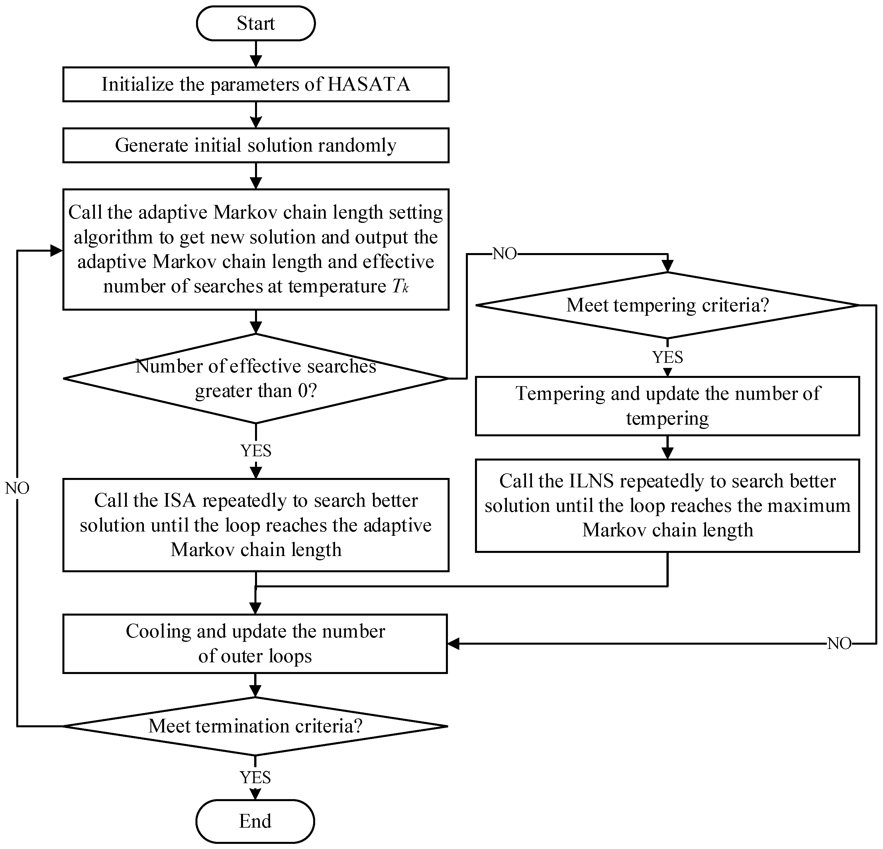
The HOMDVRP is an NP-hard problem containing path sequence optimization and vehicle-depot combination optimization problems. The simulated annealing (SA) algorithm, as a classical heuristic algorithm with excellent global search capability, has been widely used in various types of VRP [30,31]. Therefore, in this study, a hybrid adaptive simulated annealing and tempering algorithm (HASATA) based on the framework of the SA is proposed for solving the presented problem. In HASATA, we designed an improved simulated annealing (ISA) algorithm and an improved large-neighborhood search (ILNS) algorithm to enhance the search performance for the half-open path structure in HOMDVRP. Furthermore, adaptive Markov chain length and tempering mechanism are designed to improve the efficiency of the algorithm and the ability to jump out of local optimal solutions. The flowchart of HASATA is shown in Figure 2.

As shown in Figure 2, firstly, the parameters of HASATA are initialized. Secondly, initial feasible solutions are generated based on the constraints of the HOMDVRP model. Thirdly, during the pre-annealing phase, the ISA embedded in the adaptive Markov chain length setting algorithm is invoked to search for a better solution, meanwhile, the proposed algorithm outputs the effective number of searches (i.e., the number of times the current solution is updated) and the adaptive Markov chain length (also known as the number of searches in the inner layer of the algorithm), which are used as a basis for the algorithmic choices in the next step. Fourthly, if the current solution is updated at least once in the pre-annealing phase, the algorithm will enter the annealing phase and apply the ISA to search for a better solution until the loop reaches the adaptive Markov chain length; otherwise, the algorithm will enter the tempering phase and, after the tempering criterion is satisfied, the temperature is elevated and the ILNS is invoked to search in-depth until the loop reaches the maximum Markov chain length. Finally, when the algorithm reaches the number of inner adaptive searches, the temperature decreases and the number of outer iterations is updated. Steps 3 to 5 are repeated until the algorithm meets the termination criteria.

In the following sections, we describe the main procedures of the proposed HASATA in detail. The parameter symbols in the proposed algorithm and their descriptions are listed in

Table 4. The notations of the proposed algorithm.

Algorithmic Parameter	Description
$T_0$	The initial temperature
$T_{end}$	The final temperature
$T_k$	The current temperature
$\psi$	The cooling rate
$S_c$	The current solution
$S_b$	The best solution
$S_n$	The new solution
$s_k$	$\mathrm{The} \mathrm{number} \mathrm{of} \mathrm{effective} \mathrm{searches} (\mathrm{the} \mathrm{times} \mathrm{of} S_c$ is updated)
$N$	The number of tempering
$\gamma$	The tempering factor
$L_k$	The adaptive Markov chain length
$L_k^{pre}$	$\mathrm{The} \mathrm{Markov} \mathrm{chain} \mathrm{length} \mathrm{at} T_k$ in pre-annealing phase
$L_k^{max}$	The maximum Markov chain length
$H_{max}$	The outer maximum number of loops

.

3.1. Initialization of the Parameters

In the initial phase of the proposed algorithm, define the initial temperature $T_0$, the final temperature $T_{end}$, the cooling rate $\psi ,$ and the outer maximum number of loops $H_{max}$. Set the number of tempering $N$ equal to zero and define the tempering factor as $\gamma$. Define the maximum Markov chain length $L_k^{max}$. Then, define the Markov chain length at temperature $k$ in pre-annealing as $L_k^{pre}$. It usually takes the value of one-fifth of $L_k^{max}$.

3.2. Initial Solution Representation

As shown in Figure 3, for a HOMDVRP with $m$ depots and $n$ customers, since the outgoing and terminating depots of vehicle k may not coincide, we determine a vehicle path by every two neighboring depots from left to right in the coding string. Furthermore, since the number of vehicles is sufficient, we quickly generate an initial feasible solution by randomly assigning each customer $c$ to the starting and ending depots only under the consideration of vehicle loading constraints. Therefore, the encoding length of the feasible solution is $3n$.

3.3. Adaptive Markov Chain Length Mechanism

In the SA, the Markov chain length $L_k$ is also known as the number of searches in the inner layers of the algorithm at temperature $T_k$. Its value has a significant impact on the performance of the algorithm. Different from the previous empirical judgment, Li et al. [32] proposed a connection between the solution value at $T_k$ and $L_k$ and they presented an inequality for the theoretical upper bound valuation of the $L_k$ as shown in Equation (9).

$$L_k\le 4\frac{S_c-S_b}{\left|S_n-S_c\right|}$$

(9)

where $S_c$, $S_n$, and $S_b$ are the current solution, new solution, and current best solution, respectively. Here, “4” is a constant derived and has no practical significance. Therefore, the formula about $L_k$ is reformulated as shown in Equation (10).

$$L_k=\frac{S_c-S_b}{\left|S_n-S_c\right|}$$

(10)

We design an adaptive Markov chain length setting algorithm based on Equation (10), which is used to compute $L_k$ at $T_k$ while searching for a better solution. Algorithm 1 briefly explains its general structure.

Algorithm 1 The pseudo-code of adaptive Markov chain length setting algorithm
1:	Input$: S_c$$, S_b$, $T_k$, $L_k^{pre}$$, \mathrm{and} L_k^{max}$
2:	Initialization:$L_k\leftarrow 0$$; s_k\leftarrow 0$$; i\leftarrow 0$
3:	while $i\le L_k^{pre}$ do
4:	$\mathrm{Apply} \mathrm{perturbations} \mathrm{of} \mathrm{the} \mathrm{ISA} \mathrm{to} \mathrm{generate} \mathrm{new} \mathrm{solution} S_n$
5:	if $S_n<S_c$ then
6:	${ s}_k\leftarrow s_k+1$
7:	$\hspace{1em}\hspace{1em}\hspace{1em}\mathbf{if} S_n<S_b$ then
8:	$\hspace{1em}\hspace{1em}\hspace{1em}\hspace{1em}{S}_b\leftarrow S_n$
9:	end if
10:	$L_k\leftarrow L_k+\frac{S_c-S_b}{\left|S_n-S_c\right|}$
11:	$S_c\leftarrow S_n$
12:	end if
13:	else if $S_n>S_c$ and$exp\left(\frac{S_c-S_n}{T_k}\right)>random\left[0,1\right.)$ then
14:	${ s}_k\leftarrow s_k+1$
15:	$L_k\leftarrow L_k+\frac{S_c-S_b}{\left|S_n-S_c\right|}$
16:	${ S}_c\leftarrow S_n$
17:	end else if
18:	$i\leftarrow i+1$
19:	end while
20:	if $s_k>0$ then
21:	$\hspace{1em} L_k\leftarrow min\left(ceil\left(\frac{L_k}{s_k}\right),L_k^{max}\right)$
22:	end if
23:	if $s_k=0$ then
24:	$\hspace{1em} L_k\leftarrow L_k^{max}$
25:	end if
26:	Output$: S_c$$, S_b$$, L_k,$$\mathrm{and} s_k$

After initializing the parameters, $S_n$ is accepted probabilistically through the ISA with the Metropolis rule as shown in Equation (11).

$$\begin{array}{c} \\ P=\left\{\begin{array}{c}1 ,S_n-S_c<0\\ \mathit{exp}\left(\frac{-\left(S_n-S_c\right)}{T_k}\right), S_n-S_c>0\end{array}\right.\end{array}$$

(11)

Each time the $S_n$ is updated, the $s_k$ is increased by 1 (lines 6 and 14) and then Equation (10) is computed cumulatively (lines 10 and 15). At the end of the loop, if $s_k=0$, we consider the algorithm to be trapped in a local optimum and subsequently enter the tempering phase; if $s_k>0$, $L_k$ is calculated by the formula in line 21 and subsequently enter the annealing phase. Considering the fluctuation in the solution objective value in the real-world problems, we preset the maximum Markov chain length $L_k^{max}$.

3.4. Tempering Mechanism

In the tempering mechanism, if the $s_k$ equals 0, it means that the new solution will be no longer accepted. We introduce the tempering mechanism at this time to try to jump out the local optimal solution. Specifically, the temperature will rise to double the current temperature $T_k$. In addition, to avoid frequent tempering, which affects efficiency, we design the tempering criteria as shown in Equation (12) with reference to Li et al. [33].

$$\frac{S_b}{S_n+N^{\gamma }}>Random[0,1)$$

(12)

where $N$ denotes the number of tempering of HASATA and its initial value is set to zero. The index $\gamma$ of $N$ is the tempering factor and its suitable value interval is [2,5]. Imitating the Metropolis rule, in the early stage of HASATA, the tempering criteria is greatly influenced by $S_b$ and $S_n$, when $S_n$ is close to $S_b$, then it is easy to temper frequently. With the $N$ gradually increasing, in the middle and late stage of the algorithm, the tempering criteria is greatly influenced by $N$, when $N$ is large enough, the probability of tempering tends to be approximately 0. Therefore, the tempering criteria can make HASATA quickly stabilize in the late stage.

3.5. Perturbations in the ISA

Based on the SA, we add the perturbation method of depot mutation to the customer sequence perturbation for the characteristics of the half-open vehicle path structure in HOMDVRP. ISA is applied to the pre-annealing and annealing phases of the proposed algorithm to search for a better solution. The four perturbation methods designed are shown below.

(1)

Reverse: As shown in Figure 4, two customers, 1 and 3, are first randomly selected within a path and then the customer segments containing customers 1 and 3 are sorted in reverse order.

(2)

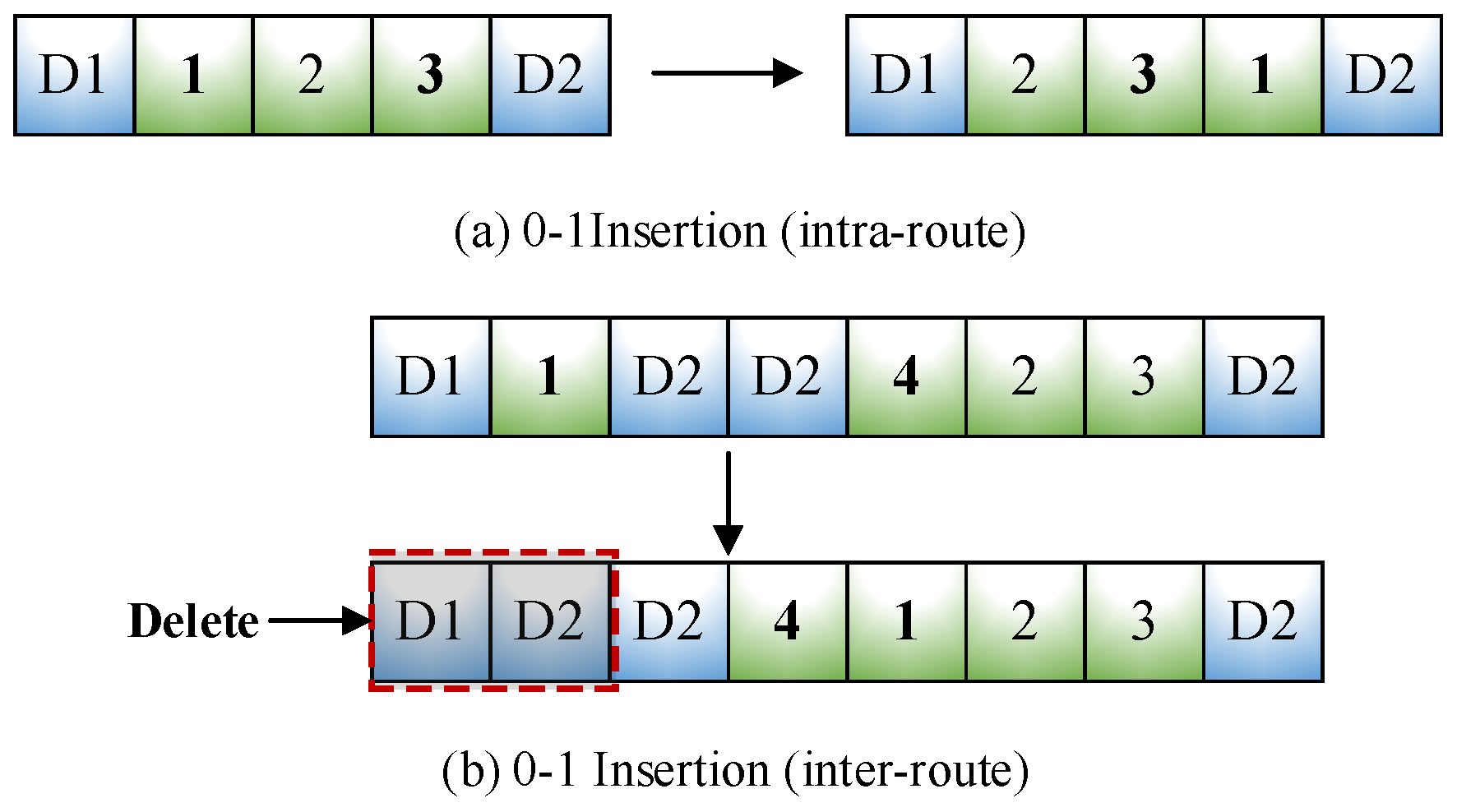
0-1 Insertion: Select two customers randomly and then insert the first selected customer to the right neighboring position of the second customer. As shown in Figure 5a, when the selected customers are all on the same path, then it is an intra-route 0-1 insertion, otherwise, it is inter-route 0-1 insertion, as shown in Figure 5b, under the premise of satisfying the vehicle load constraints, the inter-route 0-1 insertion may produce an infeasible solution situation of direct access between two depots, so after executing the inter-route 0-1 insertion, it is necessary to judge and delete the infeasible vehicle path in solution.

(3)

1-1 Exchange: Figure 6a,b shows examples of intra-route and inter-route exchanges, respectively. Notably, the inter-route 1-1 exchange needs to ensure that vehicle load constraints are not violated.

(4)

Depot mutation: in order to search for the optimal combination solution of vehicles and depots in a half-open vehicle path structure, we design the depot mutation perturbation method. As shown in Figure 7, a better solution in HOMDVRP is searched by randomly selecting a depot in a route and then replacing it with any depot in the depot set.

The procedures of the ISA are shown in Algorithm 2. The four perturbation methods mentioned above are selected by roulette to search for better solutions (lines 3–5), where the value of $L_k$ is output by Algorithm 1, which is adaptively adjusted as the algorithm converges and can therefore improve the computational efficiency of ISA.

Algorithm 2 The pseudo-code of ISA algorithm
1:	Input$: S_c$$, S_b$$, T_k$$,L_k$
2:	while $j\le L_k$   do
3:	while $S_n$ is infeasible do
4:	$S_n\leftarrow perturbation\left({\mathrm{S}}_{\mathrm{c}}\right)$
5:	end while
6:	if   $S_n<S_c$ then
7:	$S_c\leftarrow S_n$
8:	if   $S_n<S_b$ then
9:	$S_b\leftarrow S_n$
10:	end if
11:	end if
12:	else if  $S_n\ge S_c$ and$exp\left(\frac{S_c-S_n}{T_k}\right)>random\left[0,1\right.)$ then
13:	${ S}_c\leftarrow S_n$
14:	end else if
15:	$j\leftarrow j+1$
16:	end while
17:	$T_k\leftarrow \psi T_k$; $h\leftarrow h+1$
18:	if $T_k\le T_{end}$ or$h\ge H_{\mathit{m}\mathit{a}\mathit{x}}$ then
19:	Computation terminated
20:	else
21:	Turn to Algorithm 1
22:	end if
23:	Output$: S_c$$, S_b$

3.6. Destroy and Repair Operators in ILNS

The large neighborhood search (LNS) algorithm has good global search capability and is highly scalable [34,35]. Therefore, we improve the destroy and repair operators of LNS based on the features of HOMDVRP. After tempering, the local optimal solution is attempted to be jumped out by ILNS. The destroy and repair operators designed in the proposed algorithm are as follows.

The following five destroy operators are designed.

(1)

Random customer removal: this operator removes customers from the current solution at random, with the percentage of removal ranging from 0% to 10% of all customers;

(2)

Cluster removal: the operator randomly selects a customer $c$ and set $d_{max}$ as the distance between customer $c$ and its farthest neighborhood and then remove customer $c$ and all customers within its ${1/5d}_{max}$ radius;

(3)

Route removal: the operator calculates the average number of customers $\overline{n}$ across all routes, if the number of customers on a randomly selected route is greater than $\overline{n}$, then $\overline{n}$ customers will be removed randomly, otherwise, the entire route will be removed;

(4)

Relevance removal: a customer $c$ is randomly selected, then the relevance values ${Rv}_{c{c}^{\prime }}$ of customer $c$ with other customer $c^{\prime }$ are calculated by Equation (13) and finally customer c and the first $q-1$ customers with the highest relevance are removed.

$${Rv}_{c{c}^{\prime }}=1/\left(\frac{d_{c{c}^{\prime }}{\mu }_1}{{max(d}_{c{c}^{\prime }})}+X{\mu }_2\right)$$

(13)

Equation (13) is the difference degree formula and its inverse is used to represent the relevance degree. If customer $c$ is in the same route as customer $c^{\prime }$, then $X$ is 0, otherwise it is 1. ${\mu }_1$ and ${\mu }_2$ denote the weight factors, which are taken as 0.4 and 0.6, respectively.

(5)

Random depot removal: similar to the depot mutation in ISA, this operator randomly selects and records the indexes of certain warehouses and then deletes them.

To repair the infeasible solutions after being disrupted by the destroy operations, the following four repair operators are designed:

(1)

Random insertion: this operator randomly inserts a customer into an arbitrarily chosen route, and if the generated solution is not feasible, a new route is created for that customer. This operation is repeated until all customers are inserted into the route;

(2)

Sequential greedy repair: this operator randomly selects a customer from the customer pool and inserts it into the best position, then updates the current solution. Repeat this operation until all customers are inserted into the route;

(3)

Random depot repair: this operator randomly selects a depot from the pool and inserts it into the current position of the destroyed depot. Repeat this operation until all depots have been repaired;

(4)

Greedy depot repair: the operator selects a depot from the depot set and inserts it into the current position of the destroyed depot according to the principle of minimum cost increase.

The general procedure of ILNS is shown in Algorithm 3. In the fifth line of the pseudo-code, the destroy operator is performed on the current solution followed by repair (line 5). The above destroy and repair operators used are chosen by roulette. Considering the existence of both customer-specific and depot-specific operators in ILNS, we apply the destroy and repair operators for customers and depots separately in combination to ensure the effectiveness of the algorithm.

Algorithm 3 The pseudo-code of ILNS algorithm
1:	Input$: S_c$$, S_b$$, T_k$$, L_k$
2:	if meet tempering criteria then
3:	$T_k\leftarrow 2T_k$$; N\leftarrow N+1$; $q\leftarrow 0$
4:	while $q\le L_k$ do
5:	$S_n\leftarrow repair\left(destroy\left({\mathrm{S}}_{\mathrm{c}}\right)\right)$
6:	if   $S_n<S_c$ then
7:	$S_c\leftarrow S_n$
8:	if   $S_n<S_b$ then
9:	$S_b\leftarrow S_n$
10:	end if
11:	end if
12:	else if $S_n\ge S_c$ and$exp\left(\frac{S_c-S_n}{T_k}\right)>random\left[0,1\right.)$ then
13:	$S_c\leftarrow S_n$
14:	end else if
15:	$q\leftarrow q+1$
16:	end while
17:	$T_k\leftarrow \psi T_k$; $h\leftarrow h+1$
18:	if $T_k\le T_{end}$ or$h\ge H_{max}$ then
19:	Computation terminated
20:	else
21:	Turn to Algorithm 1
22:	end if
23:	else
24:	$T_k\leftarrow \psi T_k$; $h\leftarrow h+1$
25:	if $T_k\le T_{end}$ or$h\ge H_{max}$ then
26:	Computation terminated
27:	else
28:	Turn to Algorithm 1
29:	end if
30:	end if
31:	Output$: S_c$$, S_b$

3.7. Termination Criteria

In the HASATA, the tempering mechanism may result in the temperature never cooling to the $T_{end}$, which in turn prevents the algorithm from terminating the run. Therefore, in this paper, the algorithm is set to terminate the computation when the temperature reaches $T_{end}$ or the number of outer loops $H_{max}$ reaches a preset value.

4. Computational Experiments and Analysis

In this section, in order to analyze the performance of HASATA, we compare the proposed algorithm with the cardinal optimizer (COPT) [36], the hybrid adaptive large neighborhood search (HALNS) algorithm, the improved simulated annealing (ISA) algorithm, and the adaptive simulated annealing and tempering algorithm (ASATA). All the algorithms were coded in Python 3.12 and executed on 13th Gen Intel(R) Core (TM) i5-13500HX 2.50 GHz × 14 machines with 16 GB of RAM under the Windows 10 operating system.

There are 24 sets of instances generated for HOMDVRP based on the MDVRPTW instance set published by NEO (Available at http://neo.lcc.uma.es/vrp/vrp-instances/multiple-depot-vrp-with-time-windows-instances/ (accessed on 21 November 2023)). Among them, there are 12 sets for small-scale instances and 12 sets for large-scale instances. Taking instance S12-C30-D4-Q200 as an example, it implies that the small-scale 12th instance has 30 customers and 4 depot nodes and the maximum load capacity of vehicles is 200.

This section first shows the procedures for tuning the parameters. Then, we present and analyze the small-scale experimental results and large-scale experimental results.

4.1. Experiment Setting

The parameters have a large impact on the performance of meta-heuristic algorithms. Setting appropriate parameters for an algorithm can improve the optimization performance. The Taguchi analysis method is widely used as a class of statistical methods for parameter tuning, so it is adopted for the parameter tuning of HASATA.

Firstly, we select four key parameters that have the greatest impact on the proposed algorithm, which are initial temperature, cooling rate, tempering factor, and maximum Markov chain length. Then, we set low, medium, and high-level values for each of the selected parameters based on a large number of experiments to generate a table of orthogonal experiments with nine tours. Finally, we randomly selected S5-C20-D2-Q100, S12-C30-D4-Q200, L4-C50-D4-Q200, and L7-C60-D2-Q200 as sample instances and ran the algorithm 10 times with different parameter combinations to obtain the average objective value and average solution time.

Since we expect the proposed algorithm to obtain a smaller objective value in a shorter computational time, the level with the highest signal-to-noise ratio for each given parameter was determined to be the optimal level for that parameter. The alternative values for each parameter and the level that was finally chosen are listed in

Table 5. Tuning results for the parameters of HASATA.

Parameters	Low Level	Medium Level	High Level	Selected Level
$T_0$	2000	5000	8000	Low level
$\psi$	0.97	0.98	0.99	Medium level
$\gamma$	2	3	4	Medium level
$L_k^{max}$	200	250	300	Medium level

.

Overall, the initial temperature $T_0$, cooling rate $\psi$, tempering factor $\mathsf{\gamma }$, and maximum Markov chain length $L_k^{max}$ are tuned to 2000, 0.98, 3, and 250, respectively. The Markov chain length in pre-annealing $L_k^{pre}$ is set to one-fifth of $L_k^{max}$.

4.2. The Comparison Algorithms

In this section, the parameters of the comparison algorithms are introduced as follows.

COPT: It uses a branch-and-cut exact algorithm to solve mixed-integer programming models. The solver is programmed based on Python 12.1 API and we limit COPT to stop the program when the time reaches 7200 s or the memory limit is exceeded.

HALNS: The HALNS algorithm is adapted from Lahyani et al. [37]. In this paper, the initial temperature $T_0$ is set to 1000, the cooling rate $\psi ={\left(0.01/T_0\right)}^{10/{iter}_{max}}$, and the Markov chain length $L_k=20$ and the temperature is periodically reset to $T_0$ every ${iter}_{max}/10$ iterations; the rewards for updating $S_b$, $S_c$ and accepting $S_n$ are 10, 5, and 3, respectively, and the weights are updated every 200 generations.

ISA: The ISA algorithm is based on the framework of the classical simulated annealing algorithm, which uses the perturbation method designed for half-open path structures in the proposed algorithm. Its $T_0$ is set to 5000 and $\psi =$ $0.99$; $L_k=300$ and the final temperature $T_{end}=0.001$.

ASATA: The ASATA is the same parameter settings as HASATA, using perturbations instead of ILNS after tempering.

Considering the stochastic nature of the solution process of the meta-heuristic algorithms, we compare the average objective value and running time of each meta-heuristic algorithm for 20 runs in each instance.

4.3. Experimental Results of Small-Scale Instances

In this section, we compare the results of HASATA with those of the COPT solver, ISA, HALNS, and ASATA for solving 12 sets of small-scale instances. The results of the small-scale experiments shown in

Table 6. The small-scale experimental results.

Instances	COPT		HALNS			ISA			ASATA			HASATA
	${\mathbf{O}\mathbf{b}\mathbf{j}}_1$	${\mathbf{T}\mathbf{i}\mathbf{m}\mathbf{e}}_1$ (s)	${\mathbf{O}\mathbf{b}\mathbf{j}}_2$	${\mathbf{T}\mathbf{i}\mathbf{m}\mathbf{e}}_2$ (s)	${\mathbf{G}\mathbf{a}\mathbf{p}}_1$	${\mathbf{O}\mathbf{b}\mathbf{j}}_3$	${\mathbf{T}\mathbf{i}\mathbf{m}\mathbf{e}}_3$ (s)	${\mathbf{G}\mathbf{a}\mathbf{p}}_2$	${\mathbf{O}\mathbf{b}\mathbf{j}}_4$	${\mathbf{T}\mathbf{i}\mathbf{m}\mathbf{e}}_4$ (s)	${\mathbf{G}\mathbf{a}\mathbf{p}}_3$	${\mathbf{O}\mathbf{b}\mathbf{j}}_5$	${\mathbf{T}\mathbf{i}\mathbf{m}\mathbf{e}}_5$ (s)	${\mathbf{G}\mathbf{a}\mathbf{p}}_4$
S1-C10-D2-Q100	224.0	0.7	224.0	9.4	0.00%	224.0	9.5	0.00%	224.0	2.0	0.00%	224.0	5.5	0.00%
S2-C10-D4-Q100	192.0	0.4	192.1	9.9	0.05%	192.0	9.1	0.00%	192.0	1.9	0.00%	192.0	5.2	0.00%
S3-C10-D2-Q200	166.0	0.1	182.6	18.9	10.00%	166.0	5.8	0.00%	166.0	1.3	0.00%	166.0	2.4	0.00%
S4-C10-D4-Q200	161.0	0.1	173.5	15.4	7.76%	161.0	5.6	0.00%	161.0	1.3	0.00%	161.0	2.4	0.00%
S5-C20-D2-Q100	330.0	7200.0	330.5	15.5	0.15%	331.0	35.6	0.30%	333.0	6.8	0.91%	330.6	5.8	0.17%
S6-C20-D4-Q100	288.0	799.2	289.0	15.6	0.35%	289.4	25.6	0.47%	289.5	4.6	0.52%	288.2	5.9	0.07%
S7-C20-D2-Q200	262.0	6.8	262.0	22.3	0.00%	269.3	11.8	2.77%	270.1	2.5	3.09%	262.0	5.0	0.00%
S8-C20-D4-Q200	247.0	1.1	247.0	23.0	0.00%	253.2	11.7	2.49%	248.4	2.4	0.55%	247.0	4.9	0.00%
S9-C30-D2-Q100	463.0	7200.0	438.0	30.2	−5.40%	441.7	22.9	−4.60%	442.6	6.0	−4.41%	436.3	12.4	−5.78%
S10-C30-D4-Q100	361.0	7200.0	373.9	30.0	3.57%	371.7	22.4	2.95%	368.2	7.7	1.99%	361.0	14.8	0.00%
S11-C30-D2-Q200	335.0	7200.0	335.0	44.7	0.00%	344.9	15.2	2.96%	340.6	4.8	1.66%	335.0	12.9	0.00%
S12-C30-D4-Q200	309.0	126.1	310.5	44.4	0.47%	319.9	15.0	3.53%	319.0	8.8	3.24%	309.0	13.4	0.00%
Average	278.2	2477.9	279.8	23.3	1.41%	280.3	15.9	0.91%	279.5	4.2	0.63%	276.0	7.5	−0.46%

Notes: ${\mathrm{G}\mathrm{a}\mathrm{p}}_{i-1}=\left({\mathrm{O}\mathrm{b}\mathrm{j}}_i-{\mathrm{O}\mathrm{b}\mathrm{j}}_1\right)/{\mathrm{O}\mathrm{b}\mathrm{j}}_1\times 100\mathrm{\%}$, i = 2, …, 5. Bold text indicates better results for same-dimension comparisons.

verify the validity of the proposed model and algorithm.

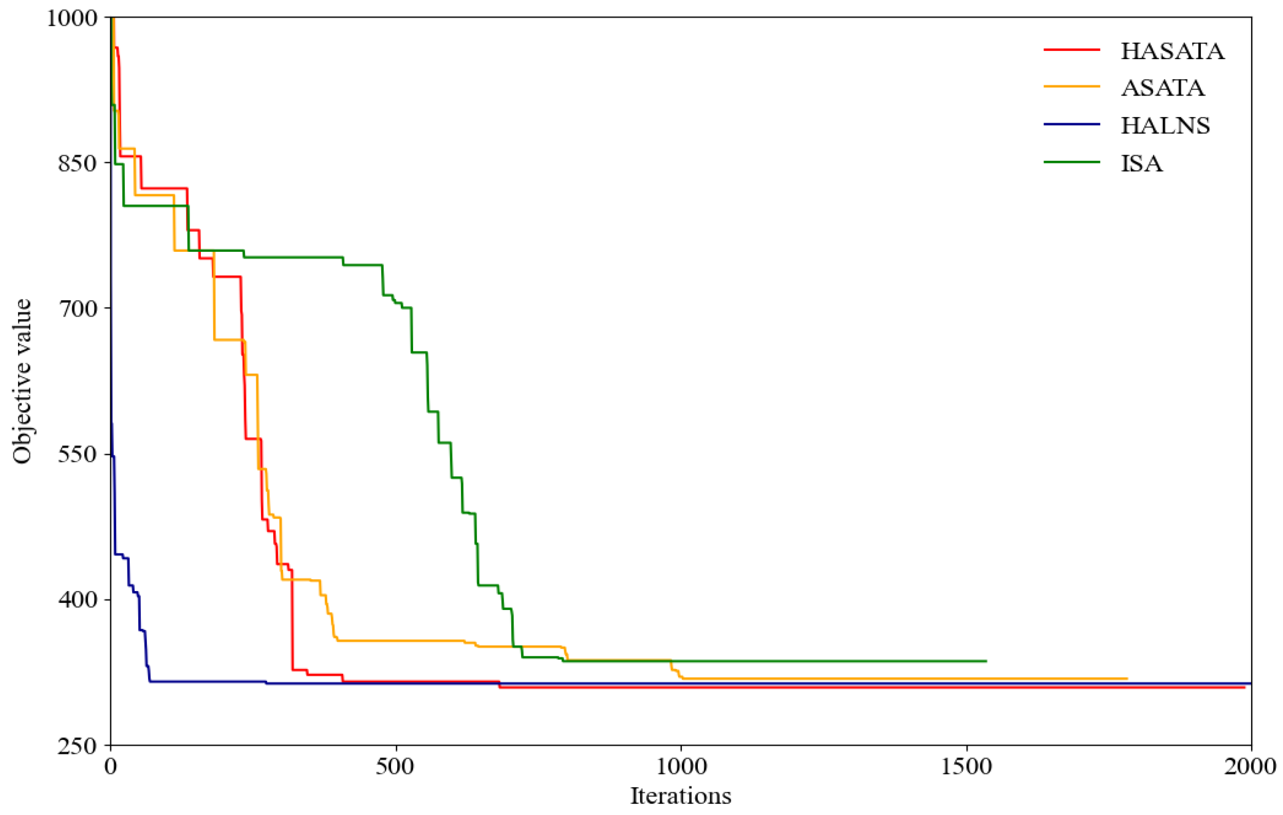
As seen from Table 6, HASATA obtains the optimal solution for 10 out of the 12 sets of small-scale arithmetic instances and its average elapsed time of 7.5 s is much lower than COPT solver’s 2477.9 s. Meanwhile, the average gap between HASATA and COPT is −0.46%, while the average gaps between HALNS, ISA and ASATA, and COPT are 1.41%, 0.91%, and 0.63%, respectively, their results are all inferior to the results given by HASATA. Moreover, it can be seen from Table 6 that the COPT solver did not find the optimal solution, for instance, S9 in 7200 s, while it took only 126.1 s to find the optimal solution for instance S12. The reason is that in the instance of the same number of customers and depot, the larger the vehicle load, the fewer vehicles are used, and it is very easy to generate feasible long-distance half-open vehicle paths. Figure 8 illustrates the optimal solution for S12, where all three paths are half-open. The convergence of the four algorithms on instance S12 is illustrated in Figure 9, where it can be seen that, compared to the other algorithms, HASATA can converge quickly in the early stage and converge to a better solution in the later stage by tempering and ILNS.

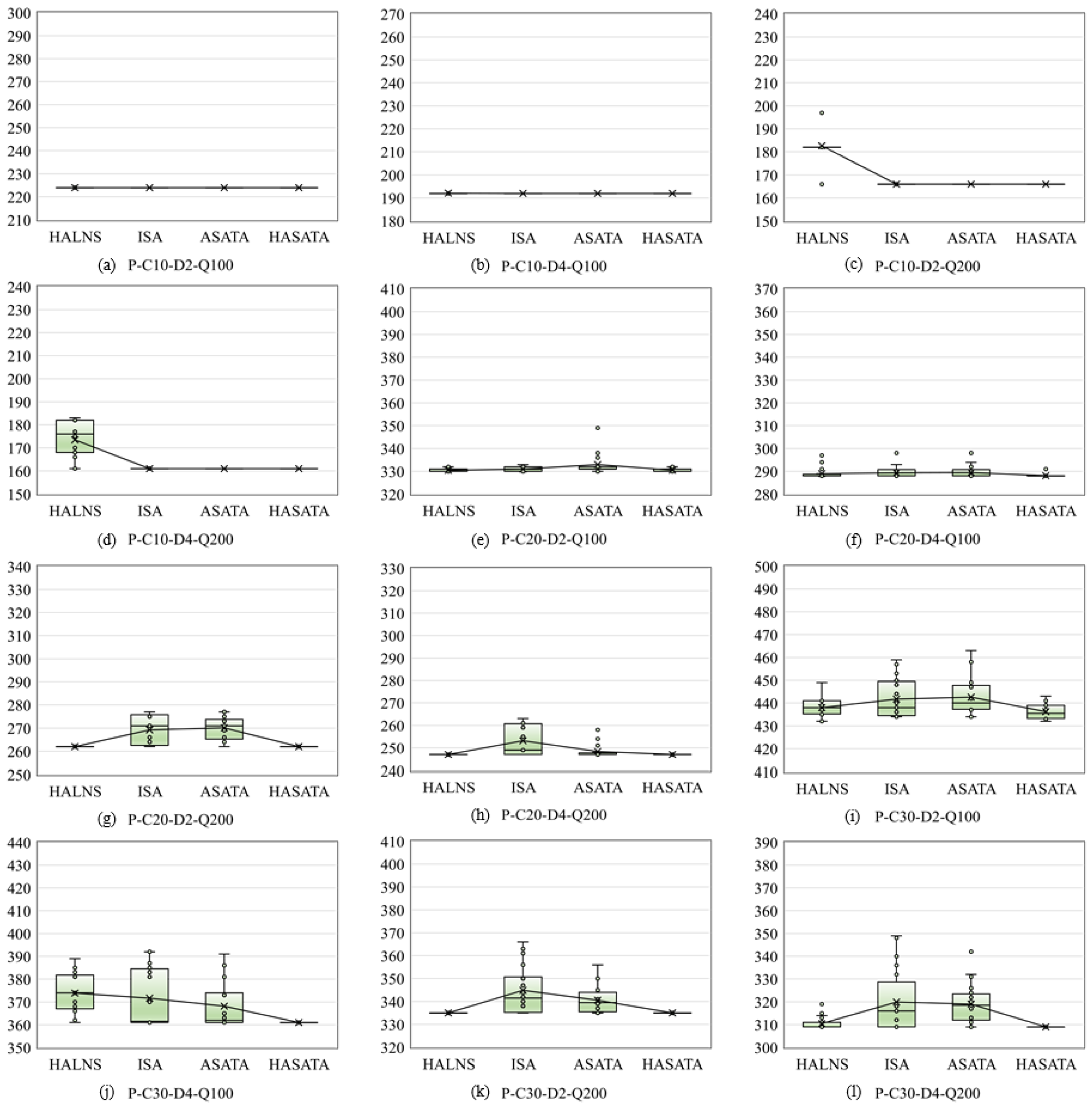
To further compare the computational stability of the four comparison algorithms, we adopt Figure 10 to show the box plots of the four algorithms for solving 12 sets of small-scale instances. From the figures, it is found that the HASATA can obtain all the optimal median values for the 12 sets of small-scale instances, while with satisfactory performance stability that significantly exceeds the comparison algorithms.

From the above analysis of the simulation results for the small-scale problem instances, the effectiveness of the proposed HASATA for solving the established HOMDVRP is verified. Meanwhile, the simulation results comparison also validates the optimization performance, computational efficiency, and performance stability of the HASATA.

4.4. Experimental Results of Large-Scale Instances

To further analyze the performance of HASATA for solving the large-scale instances of HOMDVRP, 12 groups of computational experiments are conducted.

Table 7. The large-scale experimental results.

Instances	COPT		HALNS			ISA			ASATA			HASATA
	${\mathbf{O}\mathbf{b}\mathbf{j}}_1$	${\mathbf{T}\mathbf{i}\mathbf{m}\mathbf{e}}_1$ (s)	${\mathbf{O}\mathbf{b}\mathbf{j}}_2$	${\mathbf{T}\mathbf{i}\mathbf{m}\mathbf{e}}_2$ (s)	${\mathbf{G}\mathbf{a}\mathbf{p}}_1$	${\mathbf{O}\mathbf{b}\mathbf{j}}_3$	${\mathbf{T}\mathbf{i}\mathbf{m}\mathbf{e}}_3$ (s)	${\mathbf{G}\mathbf{a}\mathbf{p}}_2$	${\mathbf{O}\mathbf{b}\mathbf{j}}_4$	${\mathbf{T}\mathbf{i}\mathbf{m}\mathbf{e}}_4$ (s)	${\mathbf{G}\mathbf{a}\mathbf{p}}_3$	${\mathbf{O}\mathbf{b}\mathbf{j}}_5$	${\mathbf{T}\mathbf{i}\mathbf{m}\mathbf{e}}_5$ (s)	${\mathbf{G}\mathbf{a}\mathbf{p}}_4$
L1-C50-D2-Q100	941.0	7200.0	635.5	58.9	−32.47%	649.4	34.9	−30.99%	658.0	14.0	−30.08%	633.8	31.6	−32.65%
L2-C50-D4-Q100	847.0	7200.0	550.0	60.9	−35.06%	547.3	33.9	−35.38%	553.6	10.8	−34.64%	528.3	34.4	−37.63%
L3-C50-D2-Q200	589.0	7200.0	482.6	76.3	−18.07%	506.8	22.5	−13.96%	521.3	7.9	−11.50%	483.1	26.1	−17.99%
L4-C50-D4-Q200	488.0	7200.0	458.6	76.8	−6.02%	468.2	22.4	−4.07%	481.2	6.6	−1.39%	452.9	27.2	−7.19%
L5-C60-D2-Q100	2044.0	7200.0	823.1	48.7	−59.73%	847.6	49.7	−58.53%	850.0	21.8	−58.41%	821.0	37.1	−59.83%
L6-C60-D4-Q100	962.0	7200.0	631.9	51.7	−34.32%	628.8	48.6	−34.64%	645.8	16.8	−32.87%	619.4	41.5	−35.62%
L7-C60-D2-Q200	1089.0	7200.0	573.0	66.9	−47.38%	599.0	31.8	−45.00%	618.1	9.4	−43.24%	579.6	29.0	−46.78%
L8-C60-D4-Q200	854.0	7200.0	526.3	67.7	−38.37%	537.5	30.3	−37.06%	547.2	8.2	−35.93%	520.2	33.8	−39.09%
L9-C70-D2-Q100	1698.0	7200.0	938.4	87.7	−44.73%	957.5	73.9	−43.61%	1002.6	17.8	−40.96%	944.9	60.1	−44.36%
L10-C70-D4-Q100	1162.0	7200.0	735.7	90.8	−36.69%	743.9	51.6	−35.98%	783.4	17.7	−32.58%	729.8	65.2	−37.19%
L11-C70-D2-Q200	1424.0	7200.0	638.7	115.6	−55.15%	688.7	33.7	−51.64%	735.3	11.5	−48.36%	647.0	51.7	−54.57%
L12-C70-D4-Q200	1041.0	7200.0	597.3	120.3	−42.63%	614.0	33.0	−41.02%	653.3	11.1	−37.25%	586.8	56.7	−43.64%
Average	1094.9	7200.0	632.6	76.9	−37.55%	649.0	38.9	−35.99%	670.8	12.8	−33.94%	628.9	41.2	−38.04%

Notes: ${\mathrm{G}\mathrm{a}\mathrm{p}}_{i-1}=\left({\mathrm{O}\mathrm{b}\mathrm{j}}_i-{\mathrm{O}\mathrm{b}\mathrm{j}}_1\right)/{\mathrm{O}\mathrm{b}\mathrm{j}}_1\times 100\mathrm{\%}$, i = 2, …, 5. Bold text indicates better results for same-dimension comparisons.

shows the results of the numerical experiments. As the problem size increases, COPT cannot obtain the optimal solution for any set of instances within 7200 s. The other four types of heuristic algorithms outperform COPT. The average gap between HALNS, ISA, ASATA, and HASATA and COPT is −37.55%, −35.99%, −33.94%, and −38.04%, respectively. The results obtained by HASATA are better than all the comparison algorithms, which obtained the eight best solutions in the 12 group experiments. Meanwhile, the average computation time of HASATA is 41.2 s, which is within the acceptable time range for all the large-scale problem instances.

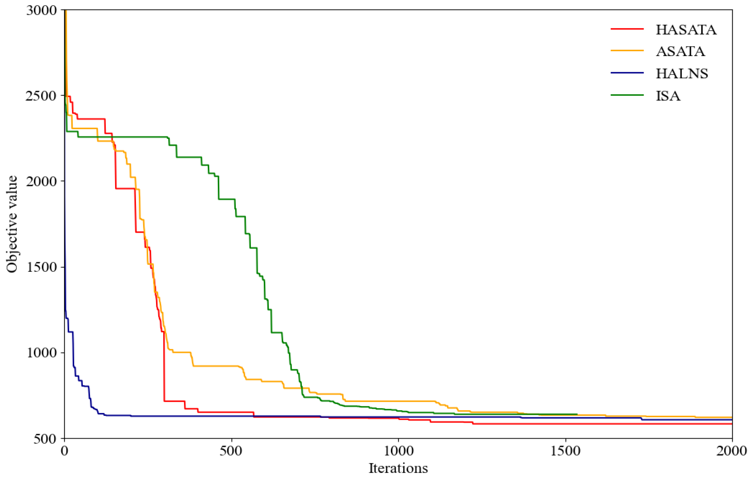
Similarly, we use Figure 11 to show the convergence of the four comparison algorithms in the large-scale instance S24, which demonstrates the convergence ability of the HASATA. It is also found that the HALNS has a good convergence ability for both the large-scale and small-scale problems. But in most of the cases, it is easier to fall into the local optimum, which is the reason that only four optimal solutions are obtained among the 12 instances. Meanwhile, the computational time of ALNS apparently exceeds that of HASATA.

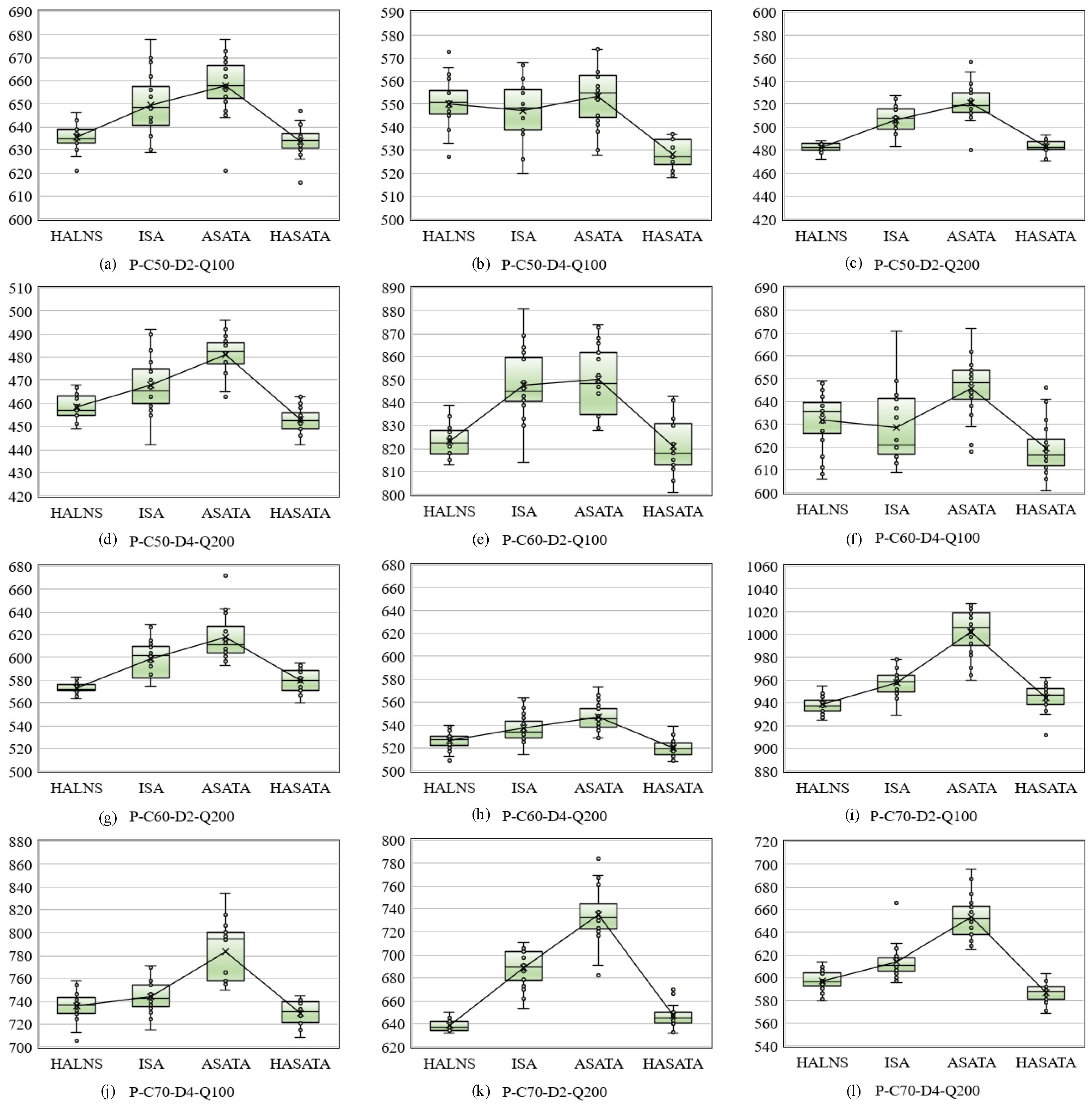
To analyze the performance stability of the HASATA for solving large-scale problem instances, we use Figure 12, which shows the box plots of the four algorithms solving 12 sets of large-scale instances.

In all of the 12 large-scale instances, HASATA outperforms the ISA and ASATA. However, in 4 sets over the 12, the HALNS outperforms the proposed HATASA, which is shown in Figure 12c,g,i,k. In the other 8 sets, the HASATA has better performance stability concerning the average value and variations. As for the computational efficiency, the HATASA outperforms the HALNS over all the large-scale instances. From the above analysis, it can be concluded that the performance stability of HATASA is satisfactory for solving the large-scale HOMDVRP.

5. Conclusions

This study aims to reduce logistics costs by studying the half-open multi-depot vehicle routing problem commonly found in collaborative logistics. Specifically, it proposes an effective hybrid meta-heuristic algorithm that is specially tailored to address the HOMDVRP with features of collaborative vehicle routing problems. To achieve this, the simulated annealing algorithm is utilized as the framework to solve the half-open multi-depot vehicle routing problem.

Firstly, a mixed-integer programming model is established to minimize the travel distance of vehicles in HOMDVRP, taking into account its features and constraints. However, due to the problem being NP-hard with a larger feasible solution space and complex problem structure, a solution representation scheme is designed based on the half-open vehicle path structure. Furthermore, the HASATA based on ISA and ILNS under the framework of SA is proposed to balance the algorithm’s breadth-search and depth-search performances. The adaptive Markov chain length and tempering mechanism are then designed to improve the computational efficiency and convergence ability of the HASATA. In the simulation experiments, 24 groups of problem instances of different scales are provided and the results verify the validity of the provided mixed-integer programming model of HOMDVRP, as well as the efficiency of the proposed HASATA for solving it. It is concluded that the HASATA outperforms all four comparison algorithms in terms of optimization performance, computational efficiency, and performance stability. Therefore, we can conclude that the provided HOMDVRP and the HASATA can generate satisfactory solutions for decision-makers in the field of collaborative logistics.

However, meta-heuristic algorithms have the characteristic of stochastic searching, so the optimization result of the proposed HASATA may vary when dealing with large-scale HOMDVRP. In addition, meta-heuristic algorithms are not problem-specific algorithms; therefore, some improved mechanisms and heuristic rules designed for HOMDVRP are incorporated into the components of HASATA in this paper. It results in the proposed algorithm requiring more parameters to be set.

In future research, benefiting from the malleability of meta-heuristic algorithms, the HASATA can be further modified to obtain better solutions in more large-scale HOMDVRP. Moreover, only the basic HOMDVRP model is considered in this study. It would be valuable to investigate the variants of the problem based on more complex collaborative logistics scenarios and apply the proposed algorithm to solve it.

References

1. Fan, H.; Sun, Y.; Yun, L.; Yu, R. A Joint distribution pricing model of express enterprises based on dynamic game theory. Mathematics 2023, 11, 4054. [Google Scholar] [CrossRef]
2. Ferrell, W.; Ellis, K.; Kaminsky, P.; Rainwater, C. Horizontal collaboration: Opportunities for improved logistics planning. Int. J. Prod. Res. 2020, 58, 4267–4284. [Google Scholar] [CrossRef]
3. Gansterer, M.; Hartl, R.F. Collaborative vehicle routing: A survey. Eur. J. Oper. Res. 2018, 268, 1–12. [Google Scholar] [CrossRef]
4. Wang, J.; Yu, Y.; Tang, J. Compensation and profit distribution for cooperative green pickup and delivery problem. Transp. Res. Part B Methodol. 2018, 113, 54–69. [Google Scholar] [CrossRef]
5. Li, J.; Wang, R.; Li, T.T.; Lu, Z.X.; Pardalos, P.M. Benefit analysis of shared depot resources for multi-depot vehicle routing problem with fuel consumption. Transp. Res. Part D Transp. Environ. 2018, 59, 417–432. [Google Scholar] [CrossRef]
6. Liu, G.; Hu, J.; Yang, Y.; Xia, S.; Lim, K.M. Vehicle routing problem in cold Chain logistics: A joint distribution model with carbon trading mechanisms. Resour. Conserv. Recycl. 2020, 156, 104715. [Google Scholar] [CrossRef]
7. Fan, H.; Yang, X.; Li, D.; Li, Y.; Liu, P.; Wu, J. Half-open multi-depot vehicle routing problem based on joint distribution mode of fresh food. Comput. Integr. Manuf. Syst. 2019, 25, 256–266. [Google Scholar] [CrossRef]
8. Zhou, Z.; Ha, M.; Hu, H.; Ma, H. Half open multi-depot heterogeneous vehicle routing problem for hazardous materials transportation. Sustainability 2021, 13, 1262. [Google Scholar] [CrossRef]
9. Wang, Y.; Ran, L.; Guan, X.; Fan, J.; Sun, Y.; Wang, H. Collaborative multicenter vehicle routing problem with time windows and mixed deliveries and pickups. Expert Syst. Appl. 2022, 197, 116690. [Google Scholar] [CrossRef]
10. Chen, Y.; Gan, H.; Chen, L. Cold chain logistics model based on joint distribution and its optimization algorithm under the background of double carbon. Control Decis. 2023, 38, 1951–1959. [Google Scholar] [CrossRef]
11. Ma, B.; Hu, D.; Chen, X.; Hu, H. An optimization of pure electric vehicle routing problem on half-open multi-distribution center. J. Transp. Syst. Eng. Inf. Technol. 2019, 19, 199–205. [Google Scholar] [CrossRef]
12. Dehghani, M.; Montazeri, Z.; Trojovská, E.; Trojovský, P. Coati Optimization Algorithm: A new bio-inspired metaheuristic algorithm for solving optimization problems. Knowl.-Based Syst. 2023, 259, 110011. [Google Scholar] [CrossRef]
13. Montazeri, Z.; Niknam, T.; Aghaei, J.; Malik, O.P.; Dehghani, M.; Dhiman, G. Golf optimization algorithm: A new game-based metaheuristic algorithm and its application to energy commitment problem considering resilience. Biomimetics 2023, 8, 386. [Google Scholar] [CrossRef] [PubMed]
14. Ho, W.; Ho, G.T.S.; Ji, P.; Lau, H.C.W. A hybrid genetic algorithm for the multi-depot vehicle routing problem. Eng. Appl. Artif. Intel. 2008, 21, 548–557. [Google Scholar] [CrossRef]
15. Venkata Narasimha, K.; Kivelevitch, E.; Sharma, B.; Kumar, M. An ant colony optimization technique for solving min–max multi-depot vehicle routing problem. Swarm Evol. Comput. 2013, 13, 63–73. [Google Scholar] [CrossRef]
16. Masmoudi, M.A.; Hosny, M.; Braekers, K.; Dammak, A. Three effective metaheuristics to solve the multi-depot multi-trip heterogeneous dial-a-ride problem. Transp. Res. Part E Logist. Transp. Rev. 2016, 96, 60–80. [Google Scholar] [CrossRef]
17. Li, J.; Pardalos, P.M.; Sun, H.; Pei, J.; Zhang, Y. Iterated local search embedded adaptive neighborhood selection approach for the multi-depot vehicle routing problem with simultaneous deliveries and pickups. Expert Syst. Appl. 2015, 42, 3551–3561. [Google Scholar] [CrossRef]
18. Braekers, K.; Caris, A.; Janssens, G.K. Exact and meta-heuristic approach for a general heterogeneous dial-a-ride problem with multiple depots. Transp. Res. Part B Methodol. 2014, 67, 166–186. [Google Scholar] [CrossRef]
19. Hesam Sadati, M.E.; Çatay, B.; Aksen, D. An efficient variable neighborhood search with tabu shaking for a class of multi-depot vehicle routing problems. Comput Oper. Res. 2021, 133, 105269. [Google Scholar] [CrossRef]
20. Montoya-Torres, J.R.; López Franco, J.; Nieto Isaza, S.; Felizzola Jiménez, H.; Herazo-Padilla, N. A literature review on the vehicle routing problem with multiple depots. Comput. Ind. Eng. 2015, 79, 115–129. [Google Scholar] [CrossRef]
21. Liu, R.; Jiang, Z.; Geng, N.; Liu, T. The half open multi-depot vehicle routing problem. J. Shanghai Jiaotong Univ. 2010, 44, 1539–1545. [Google Scholar] [CrossRef]
22. Li, J.; Li, Y.; Pardalos, P.M. Multi-depot vehicle routing problem with time windows under shared depot resources. J. Comb. Optim. 2014, 31, 515–532. [Google Scholar] [CrossRef]
23. Ge, X.; Xu, M.; Wang, X. Route optimization of urban logistics in joint distribution. Control Decis. 2016, 31, 503–512. [Google Scholar] [CrossRef]
24. Wang, Y.; Assogba, K.; Fan, J.X.; Xu, M.Z.; Liu, Y.; Wang, H.Z. Multi-depot green vehicle routing problem with shared transportation resource: Integration of time-dependent speed and piecewise penalty cost. J. Clean. Prod. 2019, 232, 12–29. [Google Scholar] [CrossRef]
25. Gu, Y.; Yuan, Y.; Zhang, L.; Duan, J. Multi-depot half open vehicle routing problem with time windows. China Mech. Eng. 2020, 13, 1733–1740. [Google Scholar] [CrossRef]
26. Fan, H.; Zhang, Y.; Tian, P.; Lv, Y.; Fan, H. Time-dependent multi-depot green vehicle routing problem with time windows considering temporal-spatial distance. Comput Oper. Res. 2021, 129, 105211. [Google Scholar] [CrossRef]
27. Fan, H.; Liu, P.; Liu, H.; Hou, D. The multi-depot vehicle routing problem with simultaneous deterministic delivery and stochastic pickup based on joint distribution. Acta Autom. Sin. 2021, 47, 1646–1660. [Google Scholar] [CrossRef]
28. Hasanpour Jesri, Z.S.; Eshghi, K.; Rafiee, M.; Van Woensel, T. The multi-depot traveling purchaser problem with shared resources. Sustainability 2022, 14, 10190. [Google Scholar] [CrossRef]
29. Bai, X.; Ma, N.; Chin, K.-S. Hybrid heuristic for the multi-depot static bike rebalancing and collection problem. Mathematics 2022, 10, 4583. [Google Scholar] [CrossRef]
30. Xiao, Y.; Konak, A. A simulating annealing algorithm to solve the green vehicle routing & scheduling problem with hierarchical objectives and weighted tardiness. Appl. Soft Comput. 2015, 34, 372–388. [Google Scholar] [CrossRef]
31. Kuo, Y. Using simulated annealing to minimize fuel consumption for the time-dependent vehicle routing problem. Comput. Ind. Eng. 2010, 59, 157–165. [Google Scholar] [CrossRef]
32. Li, Y.; Xiang, Z.; Zhang, W. A relaxation model and time complexity analysis for simulated annealing algorithm. Chin. J. Comput. 2020, 43, 16. [Google Scholar] [CrossRef]
33. Li, Y.; Jiang, W.; Xiang, Z.; Zhang, W. Relaxation model based temperature setting methods for simulated annealing algorithm. Chin. J. Comput. 2020, 43, 17. [Google Scholar] [CrossRef]
34. Ropke, S.; Pisinger, D. An adaptive large neighborhood search heuristic for the pickup and delivery problem with time windows. Transport. Sci. 2006, 40, 455–472. [Google Scholar] [CrossRef]
35. Ropke, S.; Pisinger, D. A unified heuristic for a large class of vehicle routing problems with backhauls. Eur. J. Oper. Res. 2006, 171, 750–775. [Google Scholar] [CrossRef]
36. Ge, D.; Huangfu, Q.; Wang, Z.; Wu, J.; Ye, Y. Cardinal Optimizer (COPT) User Guide. Available online: https://guide.coap.online/copt/en-doc (accessed on 18 February 2024).
37. Lahyani, R.; Gouguenheim, A.L.; Coelho, L.C. A hybrid adaptive large neighbourhood search for multi-depot open vehicle routing problems. Int. J. Prod. Res. 2019, 57, 6963–6976. [Google Scholar] [CrossRef]
Figure 1. An illustrative case for half-open multi-depot vehicle routing problem.
Mathematics 12 00947 g001
Figure 2. The flowchart of HASATA.
Mathematics 12 00947 g002
Figure 3. The initial solution representation.
Mathematics 12 00947 g003
Figure 4. Reverse.
Mathematics 12 00947 g004
Figure 5. 0-1 insertion.
Mathematics 12 00947 g005
Figure 6. 1-1 exchange.
Mathematics 12 00947 g006
Figure 7. Depot mutation.
Mathematics 12 00947 g007
Figure 8. The optimal solution for instance S12-C30-D4-Q200.
Mathematics 12 00947 g008
Figure 9. Convergence curves of the algorithms for instance S12-C30-D4-Q200.
Mathematics 12 00947 g009
Figure 10. Box plots of the results of the algorithms on the 12 small-scale instances.
Mathematics 12 00947 g010
Figure 11. Convergence curves of the algorithms for instance L12-C70-D4-Q200.
Mathematics 12 00947 g011
Figure 12. Box plots of the results of the algorithms on the 12 large-scale instances.
Mathematics 12 00947 g012