

Spatial Constraints on Economic Interactions: A Complexity Approach to the Japanese Inter-Firm Trade Network

1
Department of Computer Science, School of Computing, Tokyo Institute of Technology, Yokohama 226-8502, Japan
2
Centre for Complexity Science and Department of Mathematics, Imperial College London, London SW7 2AZ, UK
3
Department of Immunobiology, Yale University School of Medicine, New Haven, CT 06510, USA
4
Howard Hughes Medical Institute, Chevy Chase, MD 20815, USA
5
Department of Physics, Bar-Ilan University, Ramat Gan 5290002, Israel
*
Author to whom correspondence should be addressed.
Mathematics 2024, 12(8), 1244; https://doi.org/10.3390/math12081244
Submission received: 13 March 2024
/
Revised: 10 April 2024
/
Accepted: 16 April 2024
/
Published: 19 April 2024
(This article belongs to the Special Issue Modeling Real-World Problems Using Complex Networks)
Abstract
:The trade distance is an important constraining factor underpinning the emergence of social and economic interactions of complex systems. However, agent-based studies supported by the granular analysis of distances are limited. Here, we present a complexity method that places the actual geographical locations of individual firms in Japan at the epicentre of our research. By combining methods derived from network science together with information theory measures, and by using a comprehensive dataset of Japanese inter-firm business transactions, we evaluate the effects of spatial features on the structural patterns of the economy. We find that the normalised probability distributions of the distances between interacting firms obey a power law like decay concomitant with the sizes of firms and regions. Furthermore, small firms would reach large distances to become customers of large firms, while trading between either only small firms or only large firms tends to be at smaller distances. Furthermore, a time evolution analysis suggests a reduction in the overall average trading distances in last 20 years. Lastly, our analysis concerning the trading dynamics among prefectures indicates that the preference to trade with neighbouring prefectures tends to be more pronounced at rural regions as opposed to the larger central conurbations.
1. Introduction
Studies in the fields of economics and complexity science have provided valuable information on social and economic activities over the past few decades [1,2]. In very simplistic terms, economics and complexity are complementary fields. The former tends to be preoccupied with the behaviour of agents with regard to the production, consumption and distribution of wealth. In contrast, yet in tandem, the latter tends to be focused on the emerging properties of the interactions among the same agents, leading to structures such as small-world [3] or scale-free [4] networks, for example. Such agents, however, are usually located in a real physical world, and, therefore, are subject to the natural constraints of the Earth’s geography. Critically, this means that spatial features, such as transportation systems and human communication, could play a notable role in shaping the formation and structure of social and economic interactions. However, even with the best infrastructure and with interactions being facilitated by the web (virtual) world, one can hypothesise that some human, social and historical elements associated with neighbourhood and regional culture may still continue to influence trade. In this respect, our work is motivated by the fact that a robust and granular-level trade distance analysis may well provide quantitative insights into the influence of these factors at play.
To date, many studies have focused on the spatial and geographical elements of infrastructure networks—such as subways and logistics—both empirically and analytically [5,6,7,8,9,10,11,12]. However, to our knowledge, little research to date has been specifically designed to quantify the impact of space and geography on the development of real trade inter-firm networks. Instead, studies have been mostly limited to economic models based on aggregated data about properties intrinsic to agents, as opposed to granular-level data related to the interactions among these agents. A classic example of economic analysis is the transaction cost theory, proposed by Ronald H. Coase [13]. This is one of the theories that articulates the tendency of firms to gather together in specific areas, such as industrial agglomerations and industrial clusters. According to this theory, firms tend to be located close to their business partners, primarily to reduce costs—not only those easily measured, such as the transportation of goods or services, but also indirect ones, such as costs related to human communication to promote projects or make adjustments. More recently, Nakajima et al. [14] conducted an empirical study about the localisation of industries in Japan in terms of the geometric distances between the whole manufacturing firms using firm-level datasets. The distance distribution between all pairs of firms on the real network was statistically compared to that of a randomised network, and it was found that the basis of the transaction cost theory of firms did not work for every industry, since other common factors shaping the concentration of industrial activities interacted across countries. The research also confirmed that geometric distance is undoubtedly a relevant parameter for firms’ business activities. However, this work did not take the firms’ interactions—such as business transactions—into account or find any spatial distributions that resembled the form of earlier empirical studies [6,9,10,11,12].
In a complementary manner to these studies, our research is not preoccupied with the economic behaviour of agents or the associated decision-making logic and rationale. Instead, we are interested in the questions and phenomena, and we perform tests on a large available dataset from Japan in order to identify the core emerging properties of inter-firm business transaction networks. Essentially, our work attempts to address three different questions: (a) whether there is a generic functional relationship between geometric distance and the frequency of trade (hereinafter referred to as the ‘trade distance’); (b) whether distance affects trade in a uniform manner across companies of different sizes and industry activities; and (c) whether regional characteristics and patterns influence the dynamics of the trade distance. There are distinct networks that can be constructed and derived from the interactions among businesses (i.e., trading, shareholding, competition, etc.). In this research, we centre our work on the inter-firm business transaction layer related to the activities of customers and the suppliers of products and services. Within our network (namely, the ‘inter-firm trade network’), firms are represented by nodes, whereas the resulting money flows arising from the exchange of goods and services between customers and suppliers form the links (or edges) between these nodes. We note here that the general statistical properties of such networks have been the subject of extensive study [15], but without considering the trade distance dimension.
Below, we divide our study into four distinctive yet interrelated analytical methods, which are presented in Section 3, with the relevant and detailed formulae, steps and approach described in Section 2, when necessary. Firstly, we present a macro-level data analysis by providing the reader with an empirical and analytical description of the interplay and scaling relations between the structure of the inter-firm trade network, the geometric distance and the size of firms (or agents), measured by their annual sales. We follow with a second sub-section breaking down the analysis through the lens of industry sectors and prefectures, as well as adding the time dimension.
In the Section 3, we adopt traditional complexity and network randomisation methods [16] to measure and in turn highlight the impact of geometric distance on the distinctive structural features of the inter-firm trade network from a time and prefecture perspective. This is done by observing the probability distributions of the trade distances, normalised by the randomised network.
Lastly, we use the same data and randomisation methods from the previous section and transport the inter-firm trade network from the company to the prefecture level. We then make use of mutual information as a theoretical proxy measure to quantify, distinguish and classify the nature of the relationships among the prefectures [17]. This is done in order to test the hypothesis that the distinct economic fundamentals of each prefecture may influence and affect the outcomes of geometric distance trading.
2. Materials and Methods
All data used in this study are collected and provided by Teikoku Databank, Ltd. (Tokyo, Japan), one of the largest corporate research providers in Japan. It consists of corporate and business transaction data ranging from 1995 to 2021, generally encompassing over 1 million companies and over 4 million transactions per year. Whereas we carried out our analysis for all years within the above range to ensure the consistency of our findings, we present our results based on the years 2000, 2010 and 2021 as these are good representations of the evolution of the inter-firm trade network over time, as well as its core structural features.
Given the interdisciplinary nature of this research, we contextualise and explain here some of the fundamental principles and concepts underpinning our overall framework, and the reasons for selecting network science and information theory, before discussing the detailed mathematical elements.
The primary benefit of network science is that it places an emphasis on both (a) the mathematical (and the emerging statistical) properties associated with the interactions (i.e., the edges or links) between agents (i.e., nodes) and (b) the related properties associated with the agents themselves. In contrast, traditional economic and financial analyses tend to place an emphasis on the agents themselves and market aggregates. The novel aspect of our research is that all methods and analyses related to the trade distance are presented in relation to the edge associations (i.e., the trade) and not to the nodes (i.e., the firms) in isolation. When dealing with the dynamics of edge formation, the primary aim of network research is to ascertain whether the nodes are connected randomly or whether some form of attraction (i.e., preferential attachment) mechanism exists. Specifically, in this research, we focus on the strength of the role of the trade distance as a sub-component to the existing observed attraction mechanism for different combinations of company sizes. To eliminate any effects associated with the heterogeneity of the nodes, it is fundamental that the analysis is compared to the statistical properties from a configuration where the edges are generated by a random selection of nodes, but the specific properties of each node (i.e., geographical location and number of links) are maintained. This is the process applied in this study and is referred to throughout this paper as the ‘randomised network’.
Information theory—and, more specifically, mutual information I—is introduced in this study as a method to compute the level of attraction between nodes. Mathematically, I is effectively a measure of how close the observed joint distribution of two variables is to an independent joint distribution. An edge can be seen as a single observation resulting from joint distributions between target and source nodes. It follows by mathematical calculation (Equation (14)) that the pointwise mutual information formula can be adapted to the network context and be computed as the weighted divergence in the observed occurrence of an edge compared to the expected value if a specific attribute of nodes were to combine independently. In this way, the computation becomes a robust proxy to evaluate the level of attraction (for instance, the preferential attachment) between two node attributes. An additional concept within this research, the structural mutual information , corresponds to the computation of the mutual information for the randomised network.
2.1. Scaling Relations between Interacting Firms
In this subsection, all references to panels relate to those shown in Figure 1.
An individual business transaction is represented by an edge within the set of all transactions E. Two firms, a customer i and a supplier j (within the set of firms F), form a pair of nodes within a given edge.
Within panels (A) and (B), individual edges are aggregated into groups based on the annual sales S of the firms i and j,
where and .
The first panel (A) simply represents the trade frequency between the groups, i.e., the cardinality .
The second panel (B) relates to the median of the trade distance for each pairwise group . This is calculated by the Euclidean distance of the Cartesian latitude and longitude coordinates and for the pair i and j, respectively. This results in a set D containing the (converted) metric distance for all pairwise combinations , where
By construction, it follows that = ; however, ≠.
The edge aggregation for panel (C), where , and panel (D), where , follows the construct
where , , (black circles), (red triangles)}.
The normalised Mantel test , as shown in Figure 2, is computed by the following:
where is each pairwise distance of a given set D, and is the corresponding absolute difference for each pair of sales , with representing the standard deviation for each relevant set and n being the number of lengths of the sets.
We generate 10,000 random permutations of and compute a collection of to validate that the p-value < 0.001.
2.2. Geometric Proximity between Interacting Firms: Industry Sectors and Prefectures
Single edges within the set E are aggregated by paring groups of prefectures and industry categories.
In a similar manner to the edges E for a real-world network, the trade distances are calculated for each of the edges from the randomised network with the corresponding functional mapping ; see Equation (2). The randomised network is also clustered in accordance with Equation (5), resulting in equivalent groups .
For each combination , the ratio of the mean distances between the real-world and randomised networks is then calculated
Each panel of Figure 3, therefore, fixes the industry category and constitutes a histogram of the ratio for each prefecture, as calculated by Equation (6).
It follows that each datapoint within each panel represents the Cartesian coordinates for the years 2021 and 2000, respectively.
2.3. Location Dependency of Trade Distance Distribution: Prefectures and Economic Regions
Individual edges with the set E are aggregated into groups based on the prefectures and related trade distances ,
where .
The cardinality for each set is therefore the frequency of point d with the distribution frequency , which is in turn transformed into a probability density .
The same method within Equation (9) and thereafter is then applied to the randomised network set , ultimately resulting in a probability density . The ratio / therefore forms the data for Figure 4.
Figure 5 follows a similar process for the selected prefectures with the distinction that all subsets and are split into two subsets, conditional on or .
Each size of a given economic zone by the firms’ location , expressed in longitude and latitude of form i, is calculated as follows:
where N is the total number of firms and is the conversion factor from the geographical degree to the metric distance (km).
2.4. Prefectures and Communities: A Mutual Information Approach
Individual edges within set E are coarse-grained by prefecture as (customer, supplier) pairings as follows:
The probability distributions for each pairing of prefectures, the probability distribution of a prefecture being a customer and the probability distribution of a prefecture being a supplier are
noting here that the Japanese prefectures are given specific numbers, and, therefore, i and j are a range [1–47].
The pointwise contribution to the mutual information for each pair of prefectures is therefore
3. Results
3.1. Scaling Relations between Interacting Firms
The scaling relation is a fundamental tool originating from physics that is commonly used to reveal the laws governing the functional relationships between distinct, but related, physical quantities. Its application tends to lead to a better understanding of systems that have complex structures, as well as to a more comprehensible description of their inherent mechanisms. Examples are biological [19] and economic [20] systems, both of which typically reveal power law scaling behaviours. Many studies that have focused on the characteristics of firms have reported various types of scaling relations [21,22,23,24,25,26,27]. For example, it was observed that there are scaling laws in firms between the median of annual sales (million yen) S, the number of employees E, and the number of business transactions k. It has been found that and [24]. Here, we specifically analyse the scaling relations between customers and suppliers within the inter-firm trade network in order to better quantify and interpret the relations between the geometric distance and different sizes of firms. Our results are shown in four distinct panels within Figure 1.
Before delving into the analysis, we indicate here that the description of ‘customer’ and ‘supplier’ is always used for a single trade relationship, i.e., every single edge within the inter-firm trade network. A customer may be a supplier in another edge and vice versa. Moreover, the term ‘annual sales of customers’ relates to the reported annual sales of a company that are classified as a ‘customer’ in the specific edge in question. It follows that the frequency of trade refers to the cumulative number of all trades (i.e., edge) that have a customer of size and a supplier of size . In a similar manner, the median trade distance refers to the median of all trades (i.e., edges) that have a customer of size and a supplier of size .
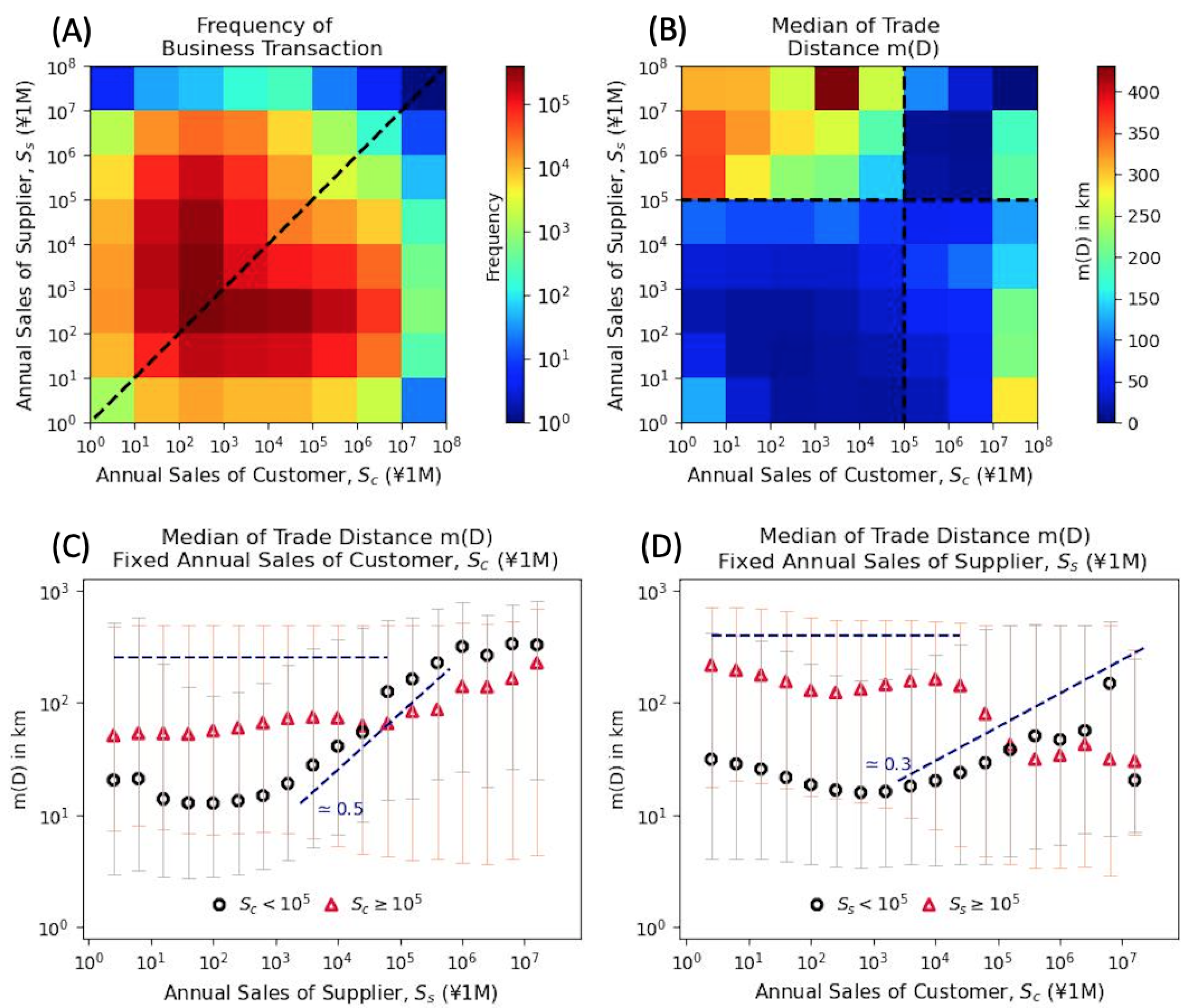
Firstly, we compare and contrast the two heatmaps at the top of Figure 1 with the methodological details described in Section 2.1. These show (A) the frequency of trades and (B) the median trade distances binned by the pairing of the annual sales of customers and those of suppliers for all existing edges within the inter-firm trade network.
It is noticeable that, whereas panel (A) is found to be almost fully symmetrical throughout the boundary , a similar pattern in panel (B) is only observed below the boundary (represented by the horizontal and vertical dotted lines). Panel (A) also highlights the existence of the relative dominance of middle-scale companies in the overall number of business transactions within the inter-firm trade network.
Following the observed abrupt break in symmetry, we classify and separate the set of edges, or business transactions, into two distinct subsets, where (black circles) and (red triangles), for the distinct roles of suppliers () in panel (C) and customers () in panel (D). From these panels, it possible to observe the existence of scaling relationships in panel (C) and in panel (D) for the firms with annual sales below the boundary , and a roughly similar inverse decay for .
Here, we emphasise that we make use of the word ‘association’ in a neutral manner and we do not imply that the individual agents, or firms, are necessarily expressing specific behaviours and preferences as a result of logical decision-making processes endogenous to the agents. Instead, we solely focus our attention on the influence of the geographical distance on the emerging properties of the inter-firm business network from a structural, and systemic, perspective.
These results seem to indicate that geometric distances tend to play a stronger role in shaping the associations (with business partners) of middle- to large-sized (or scaled) companies in comparison to small or very large companies. By considering the information across all panels, one can also suggest that large customers have a tendency to associate with small suppliers at smaller distances (average 100 km), while small customers are usually supplied by firms located at places beyond the average distance (over 200 km). In addition, it appears that the trade distances D between large companies, expressed in the upper right of panel (A) and as a tail of red triangular distributions (D), are short.
We highlight some interesting findings resulting from our analysis.
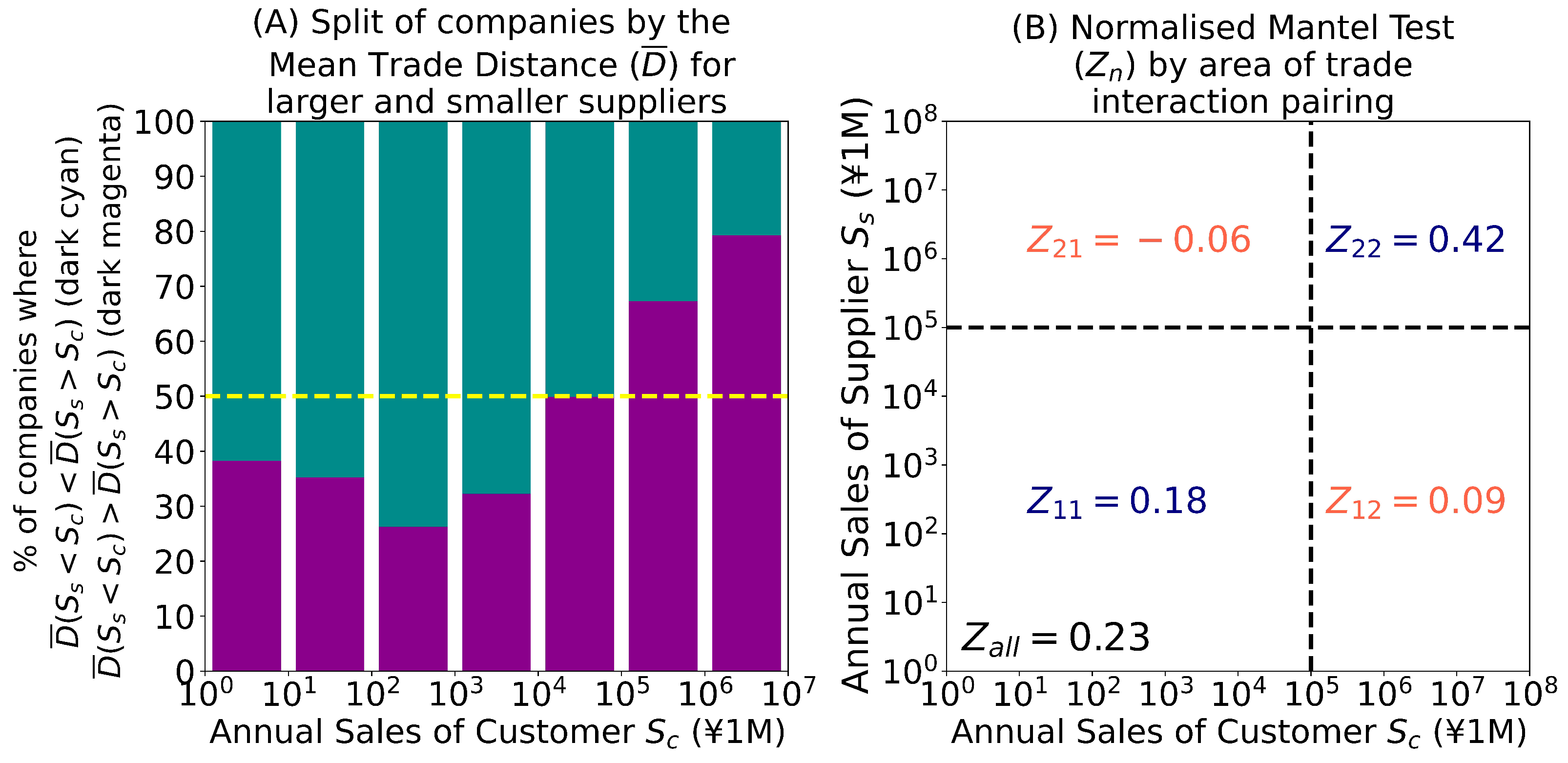
Firstly, it would be intuitive to expect that longer trade distances result in a lower frequency of trade. However, this is not a simple linear relationship. Instead, such a hypothesis will only be valid for certain combinations of sizes of customers and suppliers, with a notable asymmetric relationship where smaller customers travel long distances to trade with large suppliers but the opposite is not true. Therefore, the intricate nature of the relationships between the trade distances among companies of different sizes calls for further analysis. Figure 2 extends the analysis and provides important additional insights into the practical effects of these dynamics. In panel (A), we can observe inverse tendencies in the supplier structure between small customers () and large customers (. For around 75% to 60% of the small customers, suppliers that are smaller in relative terms () have lower average trade distances than the larger ones (), i.e., (dark cyan in panel (A)). However, this tendency reverses for large customers (increase in dark magenta proportion in panel (A)). Essentially, this means that, on average, there is a smaller benefit of cross-trading between large and small companies than inter-trading between companies of similar sizes.
To further substantiate these observations, and to reassert the general threshold of as a transition point for distinct dynamics, we have also applied the normalised Mantel test [28] (as per Equation (4)) for the whole population, as well as a subset of the four areas resulting from the combination of areas above and below the general threshold. The results shown in panel (B) clearly indicate that there is a higher level of trade distance influence for inter-trading between large companies () and, to a lesser extent, between small companies (). In contrast, the Mantel tests related to cross-sizes yield results close to zero ( and ), thereby suggesting that the trade distance plays a minimal role in shaping these combinations of customer and supplier sizes. We note here that although the Mantel test is a widely used method [29] in ecosystems to ascertain the geographical location as a potential predictor variable for species attributes, it is, in essence, a test akin to the Pearson correlation and hence subject to a number of limitations, particularly when scaling properties are present. Therefore, the values above are taken as proxies to evaluate tendencies rather than any precise and specific measure.
Despite the above, it is important to draw the reader’s attention to the fact that the overall of 0.23 suggests a limited influence (or a more localised effect from a network perspective) of the distance in shaping the inter-firm trading network. This is not surprising given that a number of studies were able to replicate inter-firm networks without the need to take into account distance as a fundamental model parameter [25,30,31]. More interestingly, studies that make use of a geographical mechanism [32] to explain network formation rely on limited data, solely from large firms. The data themselves might lead to an over-reliance on the mechanism given that it is related to a sample taken from the area where the influence is the highest, i.e., .
Secondly, from an economic analysis perspective, an interesting insight about structural competition may be obtained by the joint analysis of Figure 1 and Figure 2. As already stated, small firms tend to engage in trading with larger firms over greater distances, which is also confirmed by the Mantel tests and , nearing zero levels. However, Figure 2A implies a benefit in engaging with smaller companies (assuming the minimisation of the transport costs). We hypothesise that the main reason for such behaviour results from the fact that larger companies tend to act in markets where competition is restricted to a few players, and most of these companies are located in a few urban centres. As a result, the possibility for smaller customers to engage with local or even mid-range suppliers is severely limited.
All the above structural features can also be better understood in the context of the findings described in Section 3.4. This is because the core clusters of Tokyo and Osaka have a much smoother decay than the other clusters. In addition, larger companies—and the related transactions among these companies—are heavily concentrated within the same core clusters (of Tokyo and Osaka). For instance, 70% of large companies (whose sizes are over ) are located in Tokyo, and they account for over 50% of the business transactions between these companies. In short, the behaviour of middle-scale companies is heavily influenced by the communitarian and midway clusters, where the behaviour of larger companies is mostly shaped by the core clusters.
3.2. Geometric Proximity between Interacting Firms: Industry Sectors and Prefectures
Extensive research has been carried to evaluate industrial localisation, with several methods developed to quantify trade preferences [33,34,35]. However, these studies are based on aggregated, coarse-grained data, effectively inhibiting and limiting the analysis of the structural, systemic features of trade among businesses and firms. In any case, and unsurprisingly, the empirical results from these previous studies suggest that the geographical location of a firm is undoubtedly a relevant parameter in shaping its business partners’ trading activities. Thus far, however, to our knowledge, no study has attempted to articulate this phenomenon and quantify it by making use of comprehensive datasets that include a nationwide business transaction network. Within such an objective in mind, we attempt to observe whether geometric proximity influences, in a different manner, the generation of business interactions depending on the industry sector. Furthermore, we aim to better understand the potential evolution of trade distances over a relatively long time period (i.e., over 20 years).
Our approach within this and the subsequent sections consists of evaluating the key structural features of the real-world inter-firm trading network by normalising, comparing or contrasting it to a ‘randomised network’. The latter is synthetically built through swapping links randomly while preserving the degree distributions of each of the firms [16]. In a conceptually similar manner to other studies, we opt to maintain the degree distributions to keep the basic quantities held by the agents consistent with the network structure [17]. This approach is required since different quantities within agents (i.e., annual sales, number of employees, number of business connections) scale in a similar manner to the power law, like the degree distribution of companies. Therefore, consistency among these attributes can only be maintained if the degree distributions are kept fixed.
One method to address this issue is graph randomisation. The most commonly used such approach for biological networks is based on performing edge exchanges [4,8,9]. This algorithm (illustrated in Appendix, Figure A1 by construction preserves the network’s degree distribution exactly.
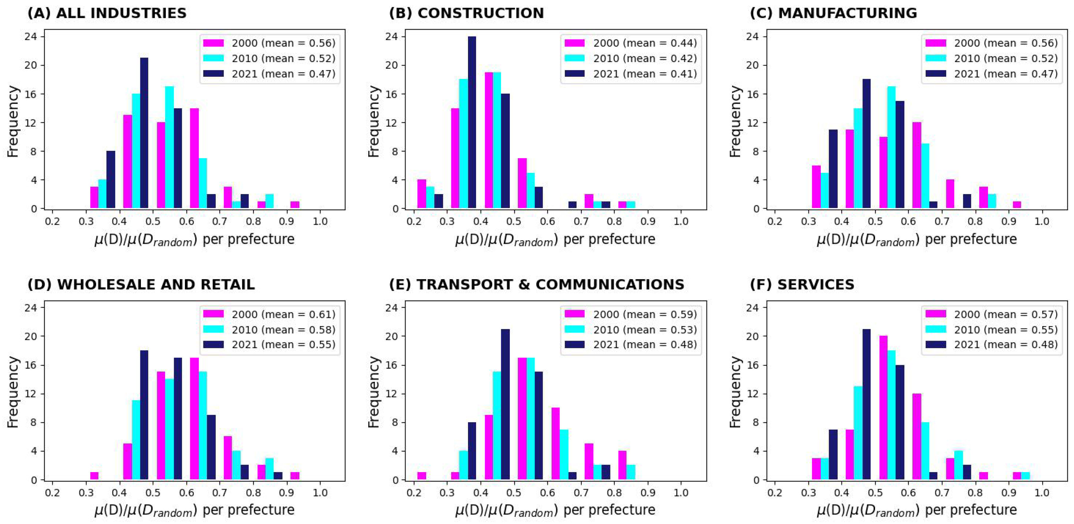
Figure 3 shows how the geometric proximity between interacting firms behaves by industry sector and is coarse-grained by prefecture for the years 2000, 2010 and 2021. Each subplot is a histogram of the frequency distribution of the Japanese prefectures as a function of the ratio for the years 2000 (pink), 2010 (cyan) and 2021 (navy blue), with the overall mean ratio for each year shown within the insets. The detailed methodology of the analysis is described in Section 2.2. These results suggest that the average trade distance for the real network D is—and has historically been—consistently and considerably shorter than that of the controlled randomised network .
Such an observation is obviously consistent with our previous findings within Figure 1, and it methodologically corroborates the empirical observation that firms tend to be influenced by their business partners’ distances when forging trade links. In addition, this analysis adds to previous factual knowledge.
Firstly, although some differences can be observed when comparing different industry sectors, these tend to be limited in nature. The construction sector (panel (B))—with the smallest ratio —tends to be the largest outlier, whereas all others, including the largest (wholesale and retail sector), tend to be fairly similar to each other.
Secondly, and interestingly, the trend over the last 21 years is the shortening of the trade distances within the real world network when normalised to the randomised network. This is a feature that can be observed in all sectors, and it is highly consistent with the theory of the growth and scaling of cities and urban environments [36].
Furthermore, we tested whether such a decrease in trading proximity with the years was related to previously existing companies or to newcomers (i.e., the growing number of new companies in each sector). This was done by reproducing the same method but only keeping links related to companies that existed in all years (i.e., 2000, 2010 and 2021). We found that the shortening of distances was related to both existing and new companies in all industries, with the sole exception of the transport and communications sector, where the reduction has been solely driven by newcomers.
We also analysed whether potentially different patterns may exist as a function of the size of firms. This was done by (a) splitting the data from the analysis in Figure 3 into two subsets related to the size of firms, where the annual sales for both customer and supplier firms were either or ; and (b) computing the mean trade distances within each subset of all edges for a given prefecture and industry for the years 2021 and 2000 (noting that all prefectures are given the same weight). We found that the average rate of decrease in the trading distance over 21 years between the largest companies () ranged from to (by industry sector), which was generally double that between smaller companies () that vary from to . This is a trend observed for all sectors, except for transport and communications, where the behaviours are similar regardless of size, revealing this again to be a contrarian sector.
3.3. Location Dependency of Trade Distance Distribution: Prefectures and Economic Regions
The statistical characteristics of the trade distance within a country will be naturally affected by the geographical shape of a given country. For example, the trade distance within Japan—an archipelago resembling a bow-shaped form—as opposed to France—a rectangular-shaped country—will fundamentally differ simply as a function of their geographical boundaries. Therefore, normalisation procedures are required in order to reduce and minimise the above effect. For the analysis of trade distance distributions, such normalisation can be done by making use of a randomised network.
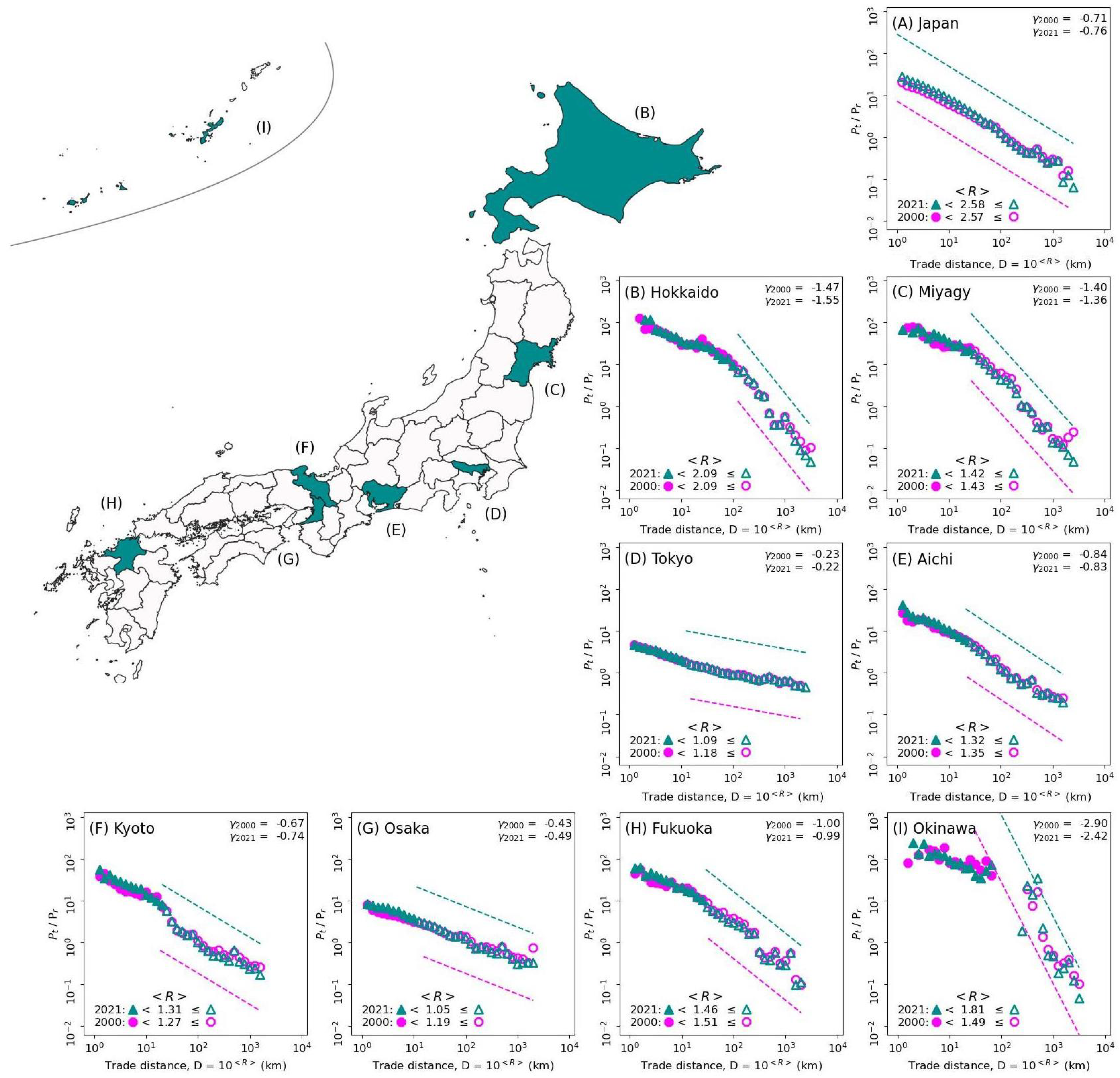
Here, we normalise the probability distribution of the link distances of a firm in the real-world inter-firm trade network by dividing each number by its equivalent probability distribution for the randomised network. In this way, we obtain the resulting normalised probability distribution within panels (A) to (I) in Figure 4. The detailed methodology is described in Section 2.3. For each of these panels, the existence of a well-approximated power law decay above a certain distance threshold can be observed, with the exponent being estimated by a process similar to the Castillo–Puig test [37,38]. In order to detect a sensible starting point for the power law decay quantitatively, we calculate each size of a given economic zone by the firms’ location , in accordance with Equations (10) and (11). Each and represent the centre of gravity and the radius of the selected prefecture, respectively.
In Figure 4, we can see the normalised probability distributions of the trade distance in (A) Japan and for firms solely located in distinct prefectures: (B) Hokkaido, (C) Miyagi, (D) Tokyo, (E) Aichi, (F) Osaka, (G) Kyoto, (H) Fukuoka and (I) Okinawa. Filled shapes (circles and triangles) show datapoints at a distance (as defined in Equation (11)), whereas empty shapes represent datapoints above the radius, where the power law decay can be effectively observed. We note that the magenta circles, representing data for 2021, almost always reside above the dark cyan triangles, related to 2000. Therefore, it is reasonable to conclude that few changes have occurred in the probability distributions of the former at a high macro level. Moreover, the power law decay above a certain distance is consistent with the statistical findings of previous studies on infrastructure networks, such as subways and logistics [5,6,7,8,9,10,11,12]. We also note that the decay exponents significantly differ between prefectures.
Furthermore, it is important to note that the shapes for urban areas, such as Tokyo and Osaka in panels (D) and (F) of Figure 4, are much flatter than others. This effectively means that the locations of firms within urban areas tend to bear little relation to the transaction costs, if one were to assume a direct link between such costs and trade distances, as advocated for by Coase’s theory of firms [13]. However, Coase’s theory may be too simplistic for the modern state of human conurbations. In order to obtain more fine-grained insights into the specific dynamics of the firm-scale dependencies between and across small, middle-sized and large firms, we generated Figure 5. The plots within the figure are similar in structure to those of Figure 4. They are distinct, however, due to the splitting of business transactions (or edges) by the threshold levels (from Figure 1) of the customer annual sales, (black circles) and (red triangles). Each panel contains the normalised probability distributions for (A) Japan as a whole; (D) Tokyo, the largest prefecture; (C) Miyagi, a small prefecture; and (H) Fukuoka, a mid-sized prefecture.
The four panels clearly indicate that the normalised probability distributions of firms both above (red triangles, ) and below (black circles, ) the threshold closely resemble each other for all prefectures at longer distances, but they have very distinctive patterns at shorter distances. By computing the best fit for the slope (in the same manner as done for Figure 4), it is possible, however, to observe that, quantitatively, the similarity increases from the largest to the smallest prefectures. Here, however, it is important to emphasise that the starting point of the fitting curve (radius km) has some impact on the exact value of the slope. The described tendency, however, is still valid, but less pronounced, if the starting point is moved to higher distances. Most importantly, larger companies tend to be much less sensitive to the distance at lower levels than smaller companies. This behaviour can be noticed in all panels within Figure 5, as the red triangles are always below the black circles at shorter distances (left side) and have a much flatter pattern. Assuming some level of validity for Coarse’s theory of firms, and by combining our observations in Figure 4 and Figure 5, we are able to conclude that, at shorter distances, small- and middle-scale firms might have stronger concerns about transaction costs than large-scale companies. However, the gap between these behaviours tends to disappear at longer distances.
It is reasonable to hypothesise that these observed dynamics may well be influenced by the high-quality infrastructure in urban areas, since most large companies are located in the core economic centres of Tokyo and Osaka. Moreover, it is important to note that the major benefits from improvements in accessibility, such as high-speed rail [39,40], may have had a ‘democratic’ effect for firms across the size spectrum. In this regard, the Japanese Shinkansen, which started its activities in 1964, may be seen as a truly beneficial transport policy, equally benefiting all firms.
3.4. Prefectures and Communities: A Mutual Information Approach
The previous section highlighted distinctive features among prefectures having different urban densities, economies and sizes. The boundaries of prefectures, however, are based upon historical administrative and geopolitical structures that might not always resemble the real trading partnerships arising from the close associations within economic structures. With this in mind, we develop a method to aggregate, or coarse-grain, prefectures into economic regions based on the existing real-world interactions within the inter-firm trade network. We then follow by comparing and contrasting the resulting distribution of the geometric trade distances for each of the regions.
Here we summarise the logic and rationale for the application of our method from a theoretical and empirical perspective. The detailed method and specific steps in developing our analysis are described within Section 2.4.
It is now well known that the distribution of nodes and edges for the Japanese inter-firm trade network follows a power law distribution governed by mechanisms associated with a cumulative advantage [16] and preferential attachment [17], leading to the formation of a disassortative network underpinned by a power law structure [36]. Previous studies show that, from an information theory perspective, an amount of mutual information that can be calculated as a function of source and target pairings will always be different from zero if the network is disassortative. Therefore, within our framework (where customers and suppliers are equivalent to sources and targets), it is possible to break down the computation of the mutual information into two separate but related components: the structural mutual information, , and the total mutual information, I. The former solely relates to the degree distribution of the nodes within a given network, whereas the latter encompasses both the node degree distribution and the disassortativeness of the network. In our research, is calculated from the randomised network, whereas I is calculated from the real-world inter-firm trade network. Such a distinction also fits well within the economics and finance perspective, since is closely related to a theoretical ‘free market’, stock-market-type configuration, where a buyer has a probability of trading with a seller solely based upon the existing quantities of stock held by the latter. In contrast, I reflects the natural market-distortion-associated dominance and influence in a real-world situation, where the ‘preferences’ of buyers and sellers are expressed.
Panels (A) and (B) of Figure 6 show, respectively, the pointwise contribution to the mutual information for the real-world inter-firm trade network and randomised network for the parings of customers (vertical) and suppliers (horizontal) by prefecture, coarse-grained in accordance with Equation (12). From analysing the structure of Equation (14), one can deduce that a positive pointwise contribution indicates that the pairing occurs in a frequency ‘higher than expectations’, whereas a negative contribution occurs with a frequency ‘below expectations’. In the context of a trading relationship, this can be interpreted as the prefectures having a higher level of attraction between the customer and supplier for the former, whereas the later shows a tendency to repel each other. From (A), three key features can be observed. Firstly, the more urbanised the prefecture (Tokyo, Osaka, Nagoya, Fukuoka), the higher the tendency to record a positive pointwise contribution to the mutual information. Secondly, as the cardinal order of prefectures is closely related to geographical proximity, it can be clearly noticed that neighbouring prefectures have a higher frequency of positive pointwise contributions (as identified visually by the shapes around the diagonal). Thirdly, the relations among prefectures (especially Tokyo) tend to be relatively symmetrical (visually, horizontal lines similar to vertical lines). In contrast, it is possible to verify from (B) that a randomised network would have kept some level of mutual information, , mainly at level of Tokyo only, the largest prefecture, with the diagonal shapes associated with the neighbourhood being effectively eliminated.
Next, we apply a clustering method where we aggregate into single trade regions all entities that have positive (in both directions) contributions to the mutual information among themselves. The clustering process starts by identifying the largest possible number of prefectures that can be fit into a single cluster with the highest levels of aggregated pointwise contribution to the mutual information , followed by segregating it, setting it aside and repeating the process with the remaining prefectures until a cluster can no longer be found. Any remaining unallocated prefectures (in our case, only Wakayama and Tochigi) are then allocated to a cluster if they contain fewer than two negative contributions between the prefecture and the cluster. The resulting clusters can be observed in the map in Figure 6.
From the analysis, a number of interesting observations can be made.
Firstly, although no geographical feature is enforced at the input level, all clusters are formed within actual geographical neighbours, and only the remote islands of Hokkaido and Okinawa remain unclustered.
Second, four clusters emerge as an exact match of Japan’s geographically defined regions, namely Kyushu (lime green), Chugoku (gold), Shikoku (saddle brown) and Tohoku (dodger blue). These clusters, together with smaller ones that we name East Chubu (darkcyan) and West Hokuriku (dim gray), make up the grouping that we define as the ‘communitarian clusters’. Importantly, as can be noted in panel (E), all communitarian clusters exhibit very similar characteristics in terms of the normalised probability distribution . It is possible to argue, therefore, that, from a structural trading perspective, these clusters have remarkable similarity, which cannot be observed at single-prefecture, administrative level.
Third, we note that a second group, the ‘core clusters’, emerges from the two urban regions associated with the two largest cities in Japan: Tokyo (East Kanto) and Osaka (West Kansai). These two clusters also show similar patterns in relation to the normalised probability distribution (panel (D)), although some limited divergence exists at shorter trade distance levels. In the previous section, and in Appendix C, we comment on the distinct patterns arising between urban prefectures and those with a lower density. By comparing and contrasting panels (D) and (E), it is possible to obtain an enhanced picture where the core (urban) clusters have dynamics fundamentally different from those of the communitarian clusters. Whereas the former tend to have a higher tendency of trade across the nation (i.e., it is flatter), the latter show a clear regional, geographically limited tendency (i.e., the decay is very pronounced).
Fourth, a third grouping, the ‘midway clusters’, encompasses two smaller clusters, namely Southeast Chubu and West Chubu and East Kansai. The prefectures within these clusters are characterised by a higher prevalence of negative contributions to the mutual information beyond Tokyo. It is also worth noting that the midway clusters are geographically located between the two largest urban centres and that the normalised probability distributions for the clusters have a hybrid shape, with characteristics close to those of the communitarian clusters at shorter distances and more similar to the core clusters at longer distances (as can be observed in panels (F) and (G)).
Fifth, panel (C) shows the computation of the pointwise contribution to the mutual information coarse-grained at the cluster level, where three general and distinct patterns can be clearly noticed depending on the grouping. The core cluster of Tokyo is generally characterised by a significant positive contribution across most of the clusters, whereas the Osaka cluster has positive contributions with clusters in Central to West Japan, but negative nearing Tokyo and North Japan. In contrast, the midway clusters tend to be negative in relation to the communitarian clusters—and between themselves—but positive in relation to the East Kanto (Tokyo) cluster. Finally, the communitarian clusters indicate a very small level of contribution among themselves, albeit with some moderate positive contributions among the neighbouring far west clusters. In brief, East Kanto has a nationwide ‘attraction’ and West Kansai ‘attracts’ the western half of the country, whereas all others have limited regional reach.
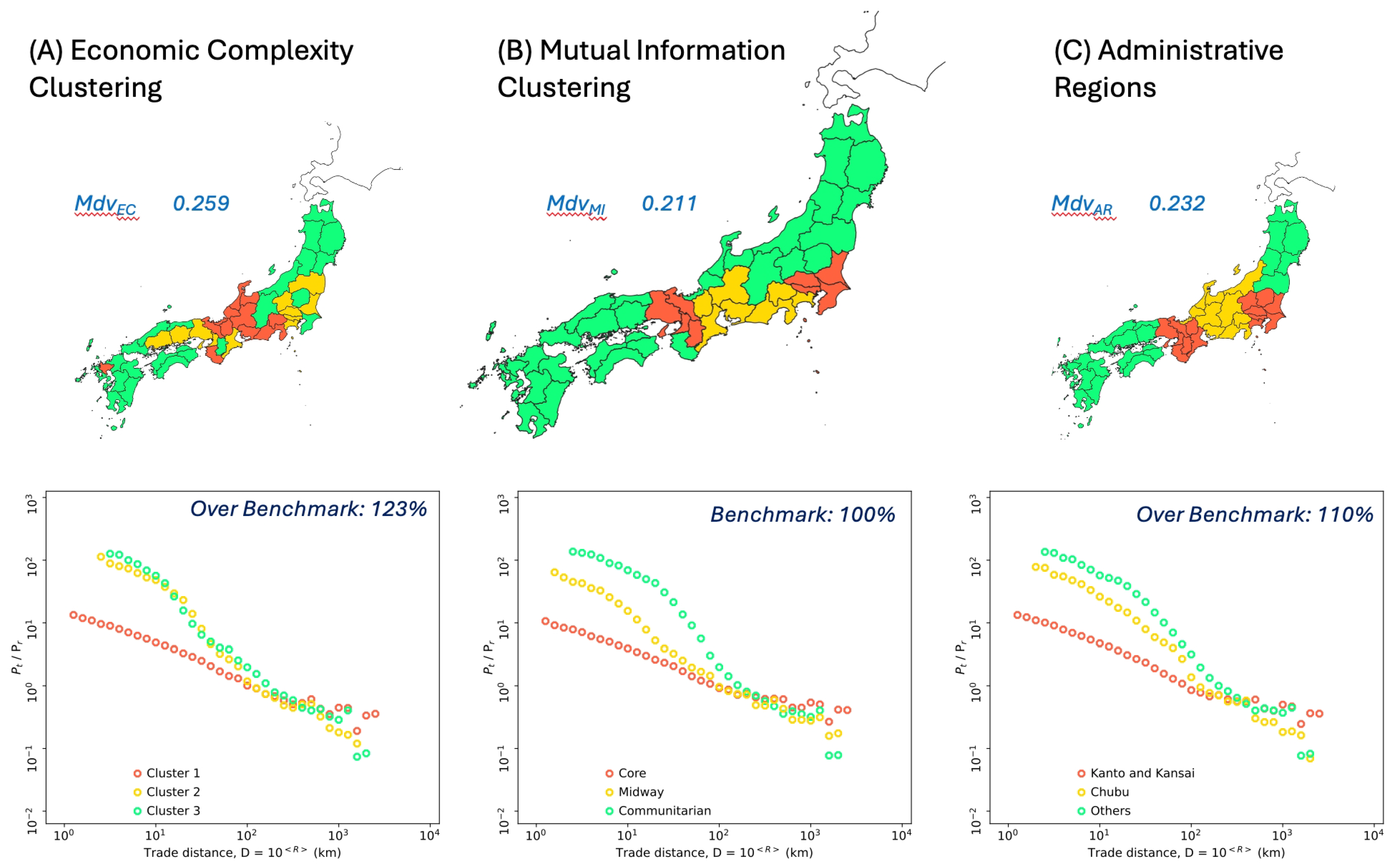
As the final component of our work, we also carried out a comparative performance analysis of our mutual information clustering approach that included (a) clustering by the minimal spanning trees (‘MST’) method, adopted for the analysis of the economic complexity of Japanese prefectures [41], and (b) clustering by the officially defined Japanese regions. We note here, however, that any choice of algorithm will yield different results based on a specific optimisation problem, and they need to be fit for the specific purpose in question. As a result, we do not claim in this research that our algorithm is superior in terms of universal performance. Instead, we simply claim that mutual information is a very valuable predictor variable to evaluate similarities in trading network structures, and that the method applied of clustering by the similarity of neighbourhood tiles yields a consistent result. Within this context, the optimisation benchmark adopted is the minimum mean deviation value of the datapoints between the actual data of the prefectures (as per Figure 4) and the equivalent aggregate curve of the clusters (as per Figure 4).
Comparing the results shown in Figure 7, we highlight three elements. Firstly, the benchmark performance shows that our mutual information approach leads to a closer alignment between the datapoints of the individual prefectures with the aggregate curve of the clusters, as expressed by the deviation values ‘Mdv’ and the percentages over the benchmark within Figure 7. Secondly, the economic complexity clustering based on MST fails to identify and distinguish the midway clusters. Thirdly, because MST is not enforced by any geographical constraint, the clustering generates a few ‘doughnuts’ (i.e., isolated prefectures), as visually illustrated by the map on the left side. We emphasise here, however, that more sophisticated methods that use mutual information as a predictor variable might yield more refined results. At the same time, the results of this analysis provide reasonable evidence that our approach is effective.
4. Discussion
As detailed within the Section 1, we designed this research to identify the core emerging properties of the inter-firm business transaction network by making use of a large, extensive and comprehensive dataset that materially encompasses all transactions within Japan.
Unsurprisingly, we found that there is a generic functional relationship between the geometric distance and frequency of trade that is largely dependent on the size of the firms within a customer and supplier relationship. Surprisingly, however, this is not a simple linear relationship as the different combinations of sizes of customers and suppliers lead to a notable asymmetric relationship between smaller customers and large suppliers. Essentially, small firms will travel large distances to partner with large suppliers. However, large firms will not travel long distances to partner with one another, as illustrated by Figure 1. We were able to identify that the observed phenomena may be the result of two different aspects. Firstly, our data analysis shows that, on average, there is less benefit in the shortening of the distances by cross-trading between large and small companies than inter-trading among companies of similar sizes. Secondly, despite such observations, smaller companies travel across long ranges to trade with large firms. We hypothesise that the main reason for such behaviour is simply the severely limited choices of smaller firms when they need to acquire products with restricted competition. This is typical of larger companies, which also tend to be located in a few urban centres.
A second finding that is somewhat counterintuitive, or against the general expectation, is the fact that when all trades among companies are taken into account and averaged, it is found that the mean distance between all customers and buyers within Japan has been decreasing over time when viewed for a relatively long period of 21 years (between 2000 and 2021). There is some level of general agreement among policymakers that, with the advances of technology and transport during the 21st century, economic and business relationships have developed a reduced dependence on geographical proximity. However, our results suggest that the trading proximity within the physical world still holds an important role in the optimisation of costs and logistics within companies (as illustrated by Figure 3), irrespective of the industry sector. Overall, our results give some evidence that technological innovation may not have substantially affected the dynamics of scaling and the pace of life in cities [36], as observed by researchers at the turn of the century.
Third, we find that the normalised probability distribution of the trade distance generally follows a shape that resembles a truncated power law distribution, both at the prefecture and trade region level—as illustrated by Figure 4, Figure 5 and Figure 6. From this narrow perspective, our results are consistent with the statistical findings of previous studies on infrastructure networks, such as subways and logistics. This suggests weaker concerns about transaction costs across shorter distances, which are predominantly considered in terms of frequency within urban areas. This is seemingly influenced by the high-quality infrastructure in urban areas, which leads to the improved efficiency and attractiveness of cities as newly connected locations with reduced communication and transaction costs.
Our work also reveals a subtle finding with regard to the influence of regional characteristics and patterns on the dynamics of the trade distance. Specifically, within Japan, we are able to clearly identify three groupings of structural trading dynamics based on their similarity (as illustrated by Figure 6): the communitarian, core and midway clusters.
The first grouping, the communitarian clusters, consists of six distinct trade regions that emerge naturally from our mutual information clustering method and that are very closely associated with the formally defined Japanese regions. The grouping is characterised by rural, lower-density areas where trading activity has a very regional, local bias (with all clusters showing a very similar, relatively high power law decay). In contrast, the core clusters are composed of the two regions around the two largest urban areas in Japan, Tokyo and Osaka, where trading distances play a much reduced role (with a much smaller power law decay). The mutual information analysis also shows clearly the distinction between these two clusters: whereas the cluster including Tokyo has a nationwide influence, Osaka’s is mostly concentrated within the western half of Japan. Lastly, the midway clusters, located between these two urban core areas, are defined by mixed characteristics, between those of the communitarian and core clusters.
Next, we discuss some of the potential consequences of the observed reduction in trade distances and speculate on existing options for policymakers. At first sight, a ‘laissez faire’ market view would conclude that the shortening of trade distances can be seen in a positive light if one were to assume that this is the result of efficient logistics, leading to some natural level of optimisation that reduces transport and commuting efforts and, by extension, emissions and pollution. However, our view is that such an argument is naive as these improvements might be simply driven by higher levels of urbanisation, instead of optimised cross-country logistics, where the second-order effects may well negate, or even worsen, any of the perceived benefits [42]. Indeed, some academics argue that middle-sized cities are experiencing an existential crisis [43] with the emergence of super-cities [36]. Therefore, we argue that our research is simply a small step towards a better understanding of the evolutionary dynamics of the trading distance and its different effects on regions. However, significant further work is required in the field to ascertain whether optimal methods can be designed to support the challenges associated with climate change (such as emissions) as well as social changes (i.e., higher deprivation, lack of opportunities, ageing population, etc., in smaller and middle-sized cities), which should take equal, if not higher, importance as economic efficiency.
In relation to the clustering method, we emphasise that mutual information is a very valuable predictor variable to evaluate similarities in trading network structures among prefectures. However, whereas the method applied of clustering by the similarity of neighbouring prefectures yields a consistent and effective result (when optimised against while maintaining reasonable similarity to the officially defined regions), it is reasonable to speculate that an approach combining additional granularity with the computation of the mutual information (by breaking prefectures down into divisions and wards) with more sophisticated clustering methods [44] may well lead to an enhanced perspective. This is an area, however, for future exploration beyond the aims of this research.
Whereas we carried out our work specifically in Japan, there is a likelihood that similar fundamental dynamics are present in most other larger countries. However, this remains a subject for future study, if similar data are available.
We also note that this study is, however, constrained by the fact that companies are not broken down into smaller sub-units such as branches. Therefore, the geographical location of a company is based on the ultimate decision-making location—normally the head office—where the management and governance of commercial transactions tend to take place (as opposed to the actual point of sale). We emphasise, though, that we do not regard this approach as a limitation, but simply a method adopted to place a focus on the decision-making centres rather than on the process-driven activities.
Author Contributions
E.V. performed and designed the experiments, interpreted the results and co-wrote the manuscript. O.L. interpreted the results and co-wrote the manuscript. S.H. designed the experiments, supervised the experimental designs, interpreted the results and reviewed the manuscript. H.T. designed the experiments, supervised the experimental designs, interpreted the results and reviewed the manuscript. M.T. conceived the project, designed the experiments, supervised the experimental designs, interpreted the results and reviewed the manuscript. All authors have read and agreed to the published version of the manuscript.
Funding
This study was partially supported by JSPS KAKENHI, Grant-in-Aid for Scientific Research (B), Grants No. 26310207.
Data Availability Statement
The data that support the findings of this study are available from Teikoku Databank, Ltd., that supported this project, but restrictions apply to the availability of these data, which were used under a license for the current study and are not publicly available. The data are, however, available from the corresponding author, M.T. (contact: [email protected]), upon reasonable request and with the permission of Teikoku Databank, Ltd.
Acknowledgments
The authors appreciate Teikoku Databank, Ltd., and the Center for TDB Advanced Data Analysis and Modeling at the Tokyo Institute of Technology for providing both the data and financial support.
Conflicts of Interest
The authors declare no conflicts of interest.
Abbreviations
The following abbreviations are used in this manuscript:
| SMI | Structural Mutual Information |
| I | Mutual Information |
| TDB | Teikoku Databank Ltd. |
Appendix A. Data Source Context and Description
Business practices in Japan have some unique features. When building relationships with clients or managing counterparty credit risks, Japanese banks and firms tend to gather a significant level of corporate information, commonly making use of professional third-party organisations to collect data and evaluate their potential and existing partners’ credit statuses. Teikoku Databank Ltd. (TDB) is one of the largest corporate research providers in Japan. The company was founded more than 120 years ago and it has been assessing the credit statuses of firms since then. TDB’s credit research reports are very extensive, including detailed information on the financial statements of firms and their history, business partners, management structures and banking transactions.
Within this research, we make use of the Japanese inter-firm business transaction networks of money transactions between customers and suppliers developed by TDB and derived from the underlying credit research activities. In addition to transactions, TDB’s database also contains the geographical coordinates of almost all firms within their domain. Therefore, the calculation of the Euclidean geometric distances among all firms becomes a relatively straightforward computational process. The database contains a register of about 1.5 million corporations with total annual sales beyond 1.4 trillion yen in 2020. Compared with the reports of the Minister of Finance in Japan and the Statistics Bureau of Japan, the database covers around 84% of the total number of corporations and about 98% of their total annual sales, with over 1 million companies with consistent and reliable information on business transactions and geographical locations.
To our knowledge, no other developed country has such an extensive and granular database held outside governmental agencies.
Appendix B. Scaling Relations between Interacting Firms
Appendix B.1. Randomised Network
We show four panels in Figure 1 to illustrate the scaling relations between customers and suppliers within the inter-firm trade network for the actual data in 2021. Here, we reproduce in Figure A1 the same graphs for the data related to the randomised network, which was generated by the process described in the Section 2.
As can be noted, the randomisation process generated results consistent with our expectations.
First, and in contrast to the actual data, the randomised data are virtually symmetrical for both the frequency of trade and the median trade distance.
Second, the median trade distance significantly increases on average as the geographic scaling is removed. This can also be observed in the panels in the lower row.
Thirdly, it can be clearly noticed that, even after normalisation, the largest firms retain a distinct pattern from the smaller firms. This is simply a result of the fact that the network is dissortative, and the numbers of edges are discrete—natural—numbers. In our research paper, we explain this feature when elaborating on the concept of the structural mutual information, SMI.
Figure A1.
The frequency of trade and distance D in a randomised network as a function of the annual sales of customers and annual sales of suppliers . (A) is a heatmap showing the frequency of trade among the and pairings, where the dotted diagonal line is the symmetry = . (B) is the equivalent heatmap quantifying the median of the and pairing, where the horizontal and vertical lines indicate the original break in symmetry for the actual data, , which is not found in the randomised network. (C) shows the scaling of the median distance of firms at different levels (above and below the actual data symmetry break) with fixed , and (D) is an equivalent plot with fixed and variable levels. Each black circle and red triangle represent firms where and , respectively. Figures are plotted on a log–log scale for the year 2021.

Appendix B.2. Actual Data for 2010
Figure A2 represents the year 2010, and it was generated on the same basis as Figure 1 (for the year 2021).
We include the year 2010 in this Appendix for a comparative analysis to show that the resulting computations for both figures are largely similar and that the break in symmetry and other trends noted in our analysis remain valid regardless of the year in question.
Figure A2.
The frequency of trade and distance D highly depend on the annual sales of customers and annual sales of suppliers for the year 2010, similarly to 2021. (A) is a heatmap showing the frequency of trade among the and pairings, where the dotted diagonal line is the symmetry = . (B) is the equivalent heatmap quantifying the the median of the and pairing, where the horizontal and vertical lines indicate the breakage of the symmetry. (C) shows the scaling of the median distance of firms at different levels (above and below the symmetry break) with fixed , and (D) is an equivalent plot with fixed and variable levels. Each black circle and red triangle represent firms where and , respectively. Figures are plotted on a log–log scale for the year 2010.

Appendix C. Correlation between the Exponents of Sizes of Economic Zones, ⟨R⟩, and the Decay γ in the Normalised Probability Distributions Pt/Pr
Figure A3 shows the exponents of the sizes of the economic zones and the power law exponent observed in the normalised probability distributions of the trade distance for each prefecture in 2021. As described in our research paper, we observe a significant level of correlation between the pairing (⟨R⟩,), which is illustrated in Figure A3 (with one outlier point).
Figure A3.
Correlation between the sizes of economic zones and the power law exponent . The figure was produced by binning the x-axis into a fixed number of datapoints (5) and calculating the averages of and within each bin. The dotted line represents the best fit line, excluding the outlier point around (1.5, −1.12).

Appendix D. Distribution of Companies across Prefectures in Japan
The maps within Figure A4 and Figure A5 are solely an illustrative reference for the reader with regard to basic company statistics in Japan.
It is worth pointing out, however,
(a) the large concentration within the Tokyo prefecture, as described in our research paper, and
(b) the fact that there is no major difference in the distribution of smaller and middle-sized firms when compared to that of the largest firms.
Figure A4.
Distribution of companies by prefecture in Japan, 2021. (A) shows the relative distribution of companies in Japan, coloured using natural numbers. In contrast, (B) shows the same distribution but colour-coded in the scale.
Figure A4.
Distribution of companies by prefecture in Japan, 2021. (A) shows the relative distribution of companies in Japan, coloured using natural numbers. In contrast, (B) shows the same distribution but colour-coded in the scale.

Figure A5.
Distribution of companies by prefecture in Japan, 2021, split by the annual sales, S. (A) shows the distribution of companies in Japan on a scale for companies with annual sales below yen, whereas (B) is the equivalent map for the companies with annual sales above yen.
Figure A5.
Distribution of companies by prefecture in Japan, 2021, split by the annual sales, S. (A) shows the distribution of companies in Japan on a scale for companies with annual sales below yen, whereas (B) is the equivalent map for the companies with annual sales above yen.

References
- Boccaletti, S.; Latora, V.; Moreno, Y.; Chavez, M.; Hwang, D.U. Complex networks: Structure and dynamics. Phys. Rep. 2006, 424, 175–308. [Google Scholar] [CrossRef]
- Schweitzer, F.; Fagiolo, G.; Sornette, D.; Vega-Redondo, F.; Vespignani, A.; White, D.R. Economic networks: The new challenges. Science 2009, 325, 422–425. [Google Scholar] [CrossRef]
- Watts, D.J.; Strogatz, S.H. Collective dynamics of ‘small-world’ networks. Nature 1998, 393, 440. [Google Scholar] [CrossRef] [PubMed]
- Barabási, A.L.; Albert, R. Emergence of scaling in random networks. Science 1999, 286, 509–512. [Google Scholar] [CrossRef]
- Rozenfeld, A.F.; Cohen, R.; Ben-Avraham, D.; Havlin, S. Scale-free networks on lattices. Phys. Rev. Lett. 2002, 89, 218701. [Google Scholar] [CrossRef]
- Yook, S.H.; Jeong, H.; Barabási, A.L. Modeling the Internet’s large-scale topology. Proc. Natl. Acad. Sci. USA 2002, 99, 13382–13386. [Google Scholar] [CrossRef]
- Xulvi-Brunet, R.; Sokolov, I.M. Evolving networks with disadvantaged long-range connections. Phys. Rev. E 2002, 66, 026118. [Google Scholar] [CrossRef]
- Barthélemy, M. Crossover from scale-free to spatial networks. EPL (Europhys. Lett.) 2003, 63, 915. [Google Scholar] [CrossRef]
- Barrat, A.; Barthelemy, M.; Pastor-Satorras, R.; Vespignani, A. The architecture of complex weighted networks. Proc. Natl. Acad. Sci. USA 2004, 101, 3747–3752. [Google Scholar] [CrossRef] [PubMed]
- Guimera, R.; Mossa, S.; Turtschi, A.; Amaral, L.N. The worldwide air transportation network: Anomalous centrality, community structure, and cities’ global roles. Proc. Natl. Acad. Sci. USA 2005, 102, 7794–7799. [Google Scholar] [CrossRef]
- Jung, W.S.; Wang, F.; Stanley, H.E. Gravity model in the Korean highway. EPL (Europhys. Lett.) 2008, 81, 48005. [Google Scholar] [CrossRef]
- Barthélemy, M. Spatial networks. Phys. Rep. 2011, 499, 1–101. [Google Scholar] [CrossRef]
- Coase, R.H. The nature of the firm. Economica 1937, 4, 386–405. [Google Scholar] [CrossRef]
- Nakajima, K.; Saito, Y.U.; Uesugi, I. Measuring economic localization: Evidence from Japanese firm-level data. J. Jpn. Int. Econ. 2012, 26, 201–220. [Google Scholar] [CrossRef]
- Takayasu, M.; Sameshima, S.; Ohnishi, T.; Ikeda, Y.; Takayasu, H.; Watanabe, K. Massive economics data analysis by econophysics methods-the case of companies’ network structure. Annu. Rep. Earth Simulator Cent. April. 2007, 2008, 263–268. [Google Scholar]
- Milo, R.; Kashtan, N.; Itzkovitz, S.; Newman, M.E.; Alon, U. On the uniform generation of random graphs with prescribed degree sequences. arXiv 2003, arXiv:cond-mat/0312028. [Google Scholar]
- Viegas, E.; Goto, H.; Kobayashi, Y.; Takayasu, M.; Takayasu, H.; Jensen, H.J. Allometric Scaling of Mutual Information in Complex Networks: A Conceptual Framework and Empirical Approach. Entropy 2020, 22, 206. [Google Scholar] [CrossRef]
- QGIS Development Team. QGIS Geographic Information System; Open Source Geospatial Foundation Project: Beaverton, OR, USA, 2019; Available online: http://qgis.osgeo.org (accessed on 18 February 2023).
- Brown, J.H.; West, G.B.; West, S.S.G.B. (Eds.). Scaling in Biology; Oxford University Press on Demand: Oxford, UK, 2000. [Google Scholar]
- Brock, W.A. Scaling in economics: A reader’s guide. Ind. Corp. Change 1999, 8, 409–446. [Google Scholar] [CrossRef]
- Takayasu, H.; Okuyama, K. Country dependence on company size distributions and a numerical model based on competition and cooperation. Fractals 1998, 6, 67–79. [Google Scholar] [CrossRef]
- Axtell, R.L. Zipf distribution of US firm sizes. Science 2001, 293, 1818–1820. [Google Scholar] [CrossRef] [PubMed]
- Fu, D.; Pammolli, F.; Buldyrev, S.V.; Riccaboni, M.; Matia, K.; Yamasaki, K.; Stanley, H.E. The growth of business firms: Theoretical framework and empirical evidence. Proc. Natl. Acad. Sci. USA 2005, 102, 18801–18806. [Google Scholar] [CrossRef]
- Watanabe, H.; Takayasu, H.; Takayasu, M. Relations between allometric scalings and fluctuations in complex systems: The case of Japanese firms. Phys. A Stat. Mech. Its Appl. 2013, 392, 741–756. [Google Scholar] [CrossRef]
- Stanley, M.H.; Amaral, L.A.; Buldyrev, S.V.; Havlin, S.; Leschhorn, H.; Maass, P.; Salinger, M.A.; Stanley, H.E. Scaling behaviour in the growth of companies. Nature 1996, 379, 804–806. [Google Scholar] [CrossRef]
- Takayasu, M.; Watanabe, H.; Takayasu, H. Generalised central limit theorems for growth rate distribution of complex systems. J. Stat. Phys. 2014, 155, 47–71. [Google Scholar] [CrossRef]
- Goto, H.; Viegas, E.; Henrik, J.J.; Takayasu, H.; Takayasu, M. Appearance of Unstable Monopoly State Caused by Selective and Concentrative Mergers in Business Networks. Sci. Rep. 2017, 7, 5064. [Google Scholar] [CrossRef] [PubMed]
- Mantel, N. The detection of disease clustering and a generalized regression approach. Cances Res. 1967, 27, 209–220. [Google Scholar]
- Jangid, K.; Whitman, W.B.; Condron, L.M.; Turner, B.L.; Williams, M.A. Soil bacterial community succession during long-term ecosystem development. Mol. Ecol. 2024, 22, 0962–1083. [Google Scholar] [CrossRef]
- Ozaki, J.; Viegas, E.; Takayasu, H.; Takayasu, M. Integration of B-to-B trade network models of structural evolution and monetary flows reproducing all major empirical laws. Sci. Rep. 2024, 1, 4628. [Google Scholar] [CrossRef] [PubMed]
- Dhyne, E.; Magerman, G.; Rubínová, S. The Belgian Production Network; Working Paper 288; National Bank of Belgium: Brussels, Belgium, 2015. [Google Scholar]
- Braha, D.; Stacey, B.; Bar-Yam, Y. Corporate competition: A self-organizing network. Soc. Netw. 2011, 33, 219–230. [Google Scholar] [CrossRef]
- Hoover, E.M. The measurement of industrial localization. Rev. Econ. Stat. 1936, 18, 162–171. [Google Scholar] [CrossRef]
- Harris, C.D. The Market as a Factor in the Localization of Industry in the United States. Ann. Assoc. Am. Geogr. 1954, 44, 315–348. [Google Scholar]
- Holmes, T.J. Localization of industry and vertical disintegration. Rev. Econ. Stat. 1999, 81, 314–325. [Google Scholar] [CrossRef]
- Bettencourt, L.M.A.; Lobo, J.; Helbing, D.; Kuhnert, C.; West, G.B. Growth, innovation, scaling, and the pace of life in cities. Proc. Natl. Acad. Sci. USA 2007, 104, 7301–7306. [Google Scholar] [CrossRef] [PubMed]
- Del Castillo, J.; Puig, P. The best test of exponentiality against singly truncated normal alternatives. J. Am. Stat. Assoc. 1999, 94, 529–532. [Google Scholar] [CrossRef]
- Malevergne, Y.; Pisarenko, V.; Sornette, D. Testing the Pareto against the lognormal distributions with the uniformly most powerful unbiased test applied to the distribution of cities. Phys. Rev. E 2011, 83, 036111. [Google Scholar] [CrossRef]
- Brócker, J.; Korzhenevych, A.; Schúrmann, C. Assessing spatial equity and efficiency impacts of transport infrastructure projects. Transp. Res. Part B Methodol. 2010, 44, 795–811. [Google Scholar] [CrossRef]
- Monzón, A.; Ortega, E.; Lxoxpez, E. Efficiency and spatial equity impacts of high-speed rail extensions in urban areas. Cities 2013, 30, 18–30. [Google Scholar] [CrossRef]
- Chakraborty, A.; Inoue, H.; ANDFujiwara, Y. Economic complexity of prefectures in Japan. PLoS ONE 2020, 15, e0238017. [Google Scholar] [CrossRef] [PubMed]
- Perera, A.T.D.; Javanroodi, K.; Mauree, D.; Nik, V.M.; Florio, P.; Hong, T.; Chen, D. Challenges resulting from urban density and climate change for the EU energy transition. Nat. Energy 2023, 8, 397–412. [Google Scholar] [CrossRef]
- Wilkinson, W. The Density Divide: Urbanization, Polarization, and Populist Backlash; Research Paper; Nishikanen Centre: Washington, DC, USA, 2012; Available online: https://www.niskanencenter.org/wp-content/uploads/2019/09/Wilkinson-Density-Divide-Final.pdf (accessed on 23 April 2023).
- Liu, Z.; Barahona, M. Graph-based data clustering via multiscale community detection. Appl. Netw. Sci. 2020, 5, 3. [Google Scholar] [CrossRef]
Figure 1.
The frequency of trade and distance D highly depends on the annual sales of customers and annual sales of suppliers . (A) is a heatmap showing the frequency trades among the and pairings, where the dotted diagonal line is the symmetry = . (B) is the equivalent heatmap quantifying the median of the and pairing, where the horizontal and vertical lines indicate the breakage of the symmetry. (C) shows the scaling of the median distance of firms at different levels (above and below the symmetry break) with fixed , and (D) is an equivalent plot with fixed and variable levels. Each black circle and red triangle represent firms where and , respectively. Figures are plotted on a log–log scale for 2021.

Figure 2.
Splitting of customers by the mean trade distance for larger and smaller suppliers and normalised Mantel tests . (A) provides a breakdown of the percentages of companies where suppliers that are smaller in relative terms () have lower average trade distances than larger ones (), i.e., (dark cyan). When the opposite occurs, , dark magenta is used for representation. (B) shows the values for the normalised Mantel test () for the whole population (black at bottom left) as well as for each subset of the four areas resulting from the combination of areas above and below the symmetry break from Figure 1.

Figure 3.
Trading proximity decreases with the years in all sectors. Industry sector analysis for geometric proximity between interacting firms, clustered by prefecture for 2000, 2010 and 2021. Each plot shows a histogram, where each prefecture is an item, for different bands as calculated by the mean trade distance within the real network and the equivalent values in the randomised network . This is done for (A) all industries and the following economic sectors: (B) construction industry, (C) manufacturing industry, (D) wholesales and retailing industries, (E) transport and communications industries and (F) services industry. Magenta, cyan and navy blue bars in each plot refer to the years 2000, 2020 and 2021, respectively. Moreover, the overall mean ratio for each year is shown within the insets for each plot.

Figure 4.
Trade distances generally follow a truncated power law at the prefecture level (generated by QGIS 3.6 software [18]). Normalised probability distributions of trade distance for each selected prefecture in 2000 and 2021, on a log–log-scale plot. Each curve of filled magenta squares, empty magenta squares, filled dark cyan circles and empty dark cyan circles shows the distribution below and above the radius for each prefecture in 2021 and 2000, respectively. The dotted lines indicate power law distributions. Each panel corresponds to the distribution generated by firms located in (A) Japan and (B) Hokkaido, (C) Miyagi, (D) Tokyo, (E) Aichi, (F) Osaka, (G) Kyoto, (H) Fukuoka and (I) Okinawa prefectures, respectively.

Figure 5.
Firms of different sizes closely resemble each other at longer distances, but have very distinctive patterns at shorter distances. Normalised probability distributions of trade distance for selected prefectures with fixed annual sales of customers (million yen) in 2021, on a log–log-scale plot. Each curve of filled shapes shows the distribution below the radius km for each prefecture in 2021, whereas non-filled shapes are datapoints above the radius. The dotted lines indicate power law distributions. Each panel contains the normalised probability distributions for (A) Japan as a whole, (C) Miyagi, (D) Tokyo and (H) Fukuoka. Each curve of black circles and red triangles shows the normalised probability of existence of a trade within distance D in 2021, categorised by the amount of annual sales of companies as and , respectively.

Figure 6.
Pointwise contributions to the mutual information and structural clustering of prefectures (generated by QGIS 3.6 software [18]). The map on the left is coloured in accordance with the eight regions that emerge from the clustering method based on the pointwise positive contribution to the mutual information. The regions are aggregated into three groupings: the communitarian clusters (E), corresponding to Kyushu (lime green), Chugoku (gold), Shikoku (saddle brown), Tohoku (dodger blue) and East Chubu (dim gray); the core clusters (D) of the Tokyo sphere (navy blue) and Osaka sphere (dark orange); and the midway clusters (F) (dark magenta). The panels in the bottom row show the normalised probability distributions with distance (similarly to Figure 5), where panel (G) is a schematic trend-line representation of the three groupings. Panels (A), (B) and (C) present the heatmaps of the pointwise contributions to the mutual information (calculated in accordance with Equation (14)) for the real world inter-firm trade network, the randomised network and the clustered regions, respectively.

Figure 7.
Comparative structural clustering of prefectures by distinct methods (generated by QGIS 3.6 software [18]). The three maps at the top are coloured in accordance with the three highest-order clusters that emerge from each clustering method: the economic complexity (A), the method applied in this research (i.e., the mutual information) (B) and the officially defined administrative regions (C). The colour coding is related to the clusters identified by the legends within the panels below. The panels at the bottom show the normalised probability distributions with distance (similarly to Figure 5).

Disclaimer/Publisher’s Note: The statements, opinions and data contained in all publications are solely those of the individual author(s) and contributor(s) and not of MDPI and/or the editor(s). MDPI and/or the editor(s) disclaim responsibility for any injury to people or property resulting from any ideas, methods, instructions or products referred to in the content. |
© 2024 by the authors. Licensee MDPI, Basel, Switzerland. This article is an open access article distributed under the terms and conditions of the Creative Commons Attribution (CC BY) license (https://creativecommons.org/licenses/by/4.0/).
Share and Cite
MDPI and ACS Style
Viegas, E.; Levy, O.; Havlin, S.; Takayasu, H.; Takayasu, M. Spatial Constraints on Economic Interactions: A Complexity Approach to the Japanese Inter-Firm Trade Network. Mathematics 2024, 12, 1244. https://doi.org/10.3390/math12081244
AMA Style
Viegas E, Levy O, Havlin S, Takayasu H, Takayasu M. Spatial Constraints on Economic Interactions: A Complexity Approach to the Japanese Inter-Firm Trade Network. Mathematics. 2024; 12(8):1244. https://doi.org/10.3390/math12081244
Chicago/Turabian StyleViegas, Eduardo, Orr Levy, Shlomo Havlin, Hideki Takayasu, and Misako Takayasu. 2024. "Spatial Constraints on Economic Interactions: A Complexity Approach to the Japanese Inter-Firm Trade Network" Mathematics 12, no. 8: 1244. https://doi.org/10.3390/math12081244
Note that from the first issue of 2016, this journal uses article numbers instead of page numbers. See further details here.