Urban Origin–Destination Travel Time Estimation Using K-Nearest-Neighbor-Based Methods

Abstract

Improving the estimation of origin–destination (O-D) travel times poses a formidable challenge due to the intricate nature of transportation dynamics. Current deep learning models often require an overwhelming amount of data, both in terms of data points and variables, thereby limiting their applicability. Furthermore, there is a scarcity of models capable of predicting travel times with basic trip information such as origin, destination, and starting time. This paper introduces novel models rooted in the k-nearest neighbor (KNN) algorithm to tackle O-D travel time estimation with limited data. These models represent innovative adaptations of weighted KNN techniques, integrating the haversine distance of neighboring trips and incorporating correction factors to mitigate prediction biases, thereby enhancing the accuracy of travel time estimations for a given trip. Moreover, our models incorporate an adaptive heuristic to partition the time of day, identifying time blocks characterized by similar travel-time observations. These time blocks facilitate a more nuanced understanding of traffic patterns, enabling more precise predictions. To validate the effectiveness of our proposed models, extensive testing was conducted utilizing a comprehensive taxi trip dataset sourced from Santiago, Chile. The results demonstrate substantial improvements over existing state-of-the-art models (e.g., MAPE between 35 to 37% compared to 49 to 60% in other methods), underscoring the efficacy of our approach. Additionally, our models unveil previously unrecognized patterns in city traffic across various time blocks, shedding light on the underlying dynamics of urban mobility.

1. Introduction

In our increasingly interconnected world, the efficient movement of people and goods is essential for economic growth and quality of life. Origin–destination travel times serve as the backbone of multiple transportation planning and management models. For example, urban planners and policymakers rely on these estimates to design and improve transportation networks, allocate resources, and implement infrastructure projects, as accurate travel-time estimates can reveal trends and patterns in transportation behavior, aiding in the development of long-term sustainable urban strategies. In congested urban areas, accurate travel-time estimates also empower traffic management systems and help improve public transit by aligning traffic patterns with traffic signal control systems and transit schedules and routes.

Estimation of origin–destination (O-D) travel times is a complex task that involves various methods and approaches that have evolved. The simplest approach is to establish a mathematical relationship between travel time and distance (considering factors such as road type, speed limits, and congestion). Other models use historical data to develop indices that reflect travel time variations based on time of day, day of the week, or specific events (e.g., holidays or special occasions), and then travel time indices are used to adjust base travel-time estimates. For example, given the data collected from a sample of travelers on their trips (origin, destination, departure time, and arrival time), the average and variability of the travel time can be calculated.

The proliferation of GPS-equipped smartphones has provided a rich source of real-time travel data. Mobile applications and GPS navigation systems record the travel times of individual vehicles, which can be aggregated and analyzed to estimate travel times on specific routes and at specific times. However, there are cases where there is only partial information on the GPS data due to insufficient information (sample size) or low coverage. In these cases, only certain traces or only location or departure/arrival times are available. This is also the case for public crowd-sourced data. Public data from platforms such as Waze, Uber, or Google Maps usually provide only location and departure/arrival times. In these cases, as mentioned in [1], advanced machine learning techniques, which can account for complex interactions and non-linearities in traffic patterns, can be trained on historical traffic data to predict O-D travel times.

In this paper, we examine the O-D time estimation problem, where partial information is available: the origin and destination location and the time of day when the trip is scheduled are considered to estimate the travel time. This problem arises from the estimation of travel time for taxi rides within a city that report their GPS location for passenger trips [1]. Given the large volume of data generated in this kind of context, we resort to machine learning tools to generate time predictions. In particular, the focus is on the KNN method, one of the most popular methods in the field [2], which uses travel-time observations from a training set that is similar to the one to be estimated. To produce high-quality estimations, extensions and improvements to the KNN model are proposed, addressing shortcomings of this model for estimating O-D travel times. Our contributions are the following:

• We propose the haversine metric as a new distance metric for KNN. This metric enables the elimination of bias inherent in the commonly used Euclidean distance. Additionally, we include a correction factor for the KNN’s estimated times, adjusting predictions based on the distances traveled by the KNNs.
• An adaptive algorithm is proposed to efficiently partition the neighbor search based on the trip’s starting time. Employing a binary search approach, the algorithm generates time partitions to define the training observation neighbors. This method facilitates the inclusion of a new predictor variable in the model without necessitating adjustments to the distance metric. This extension to the KNN framework enables the incorporation of additional input variables into the model.
• Finally, a comprehensive computational study was conducted using a taxi company database to examine methods and algorithms commonly utilized in machine learning. The results and analysis offer meaningful insights into the times (hours) of the day exhibiting the most similar travel times. These insights are deemed potentially valuable to decision-makers.

The remainder of the paper is organized as follows. Section 2, discusses the relevant literature. Section 3 formally defines the O-D travel time estimation problem, while in Section 4, improvements to the KNN and the algorithm for partitioning the travel starting time are described. The results of a comprehensive computational study are shown and analyzed in Section 5. Finally, the conclusions are presented in Section 6.

2. Literature Review

Traditionally, travel time estimation has used simple models based on average speeds or historical data [3]. However, these methods often fail to capture real-time variations caused by traffic congestion, road conditions, and unforeseen incidents. With the advent of advanced technologies and the proliferation of data sources, there is a growing opportunity to leverage partial data to develop more accurate and dynamic travel time estimation models. One of the primary sources of partial data for the estimation of travel time is the Global Positioning System (GPS). GPS devices or smartphone applications equipped with GPS capabilities provide location information that can be used to track the movement of vehicles. By analyzing the trajectory data collected from these GPS devices, it becomes possible to extract valuable insights regarding travel times [4,5,6], speeds [7,8], congestion patterns on specific routes [9,10,11], or destination choices [12].

The development of sophisticated algorithms, such as machine learning models and data fusion approaches has opened up new possibilities to estimate travel times with multiple data sources. While there have been multiple approaches proposed over the years, the state of the art can be roughly separated into two different approaches: models using trajectory data and models using partial data.

2.1. Travel Time Prediction Using Trajectory Data

GPS trajectory data usually consists of millions of data points that are useful for deep learning models. Currently, GPS update rates are around one update per second. Then, even for short trips of 20 min, GPS trajectory data generate over a thousand data points. This vast amount of generated data has fueled the application of deep learning models to this type of data. For example, Chughtai et al. [13] tested four neural network models (convolutional neural networks, multilayer perceptron, long short-term memory, and gated recurrent unit) and a hybrid ensemble to predict travel times with trajectory data. Vankdoth and Arock [14] used a hybrid model, combining a U-net and graph neural network, to predict traffic flow, and used it to estimate the travel time from one location to another. Sheng et al. [15] used an image-processing method (the image is generated using GPS data) and time series for travel time prediction on taxi and online ride-hailing. Li Zhuang and Wong [16] used multiple source data in combination with a long short-term memory module (for extracting temporal features) and a convolutional neural network module (for extracting spatial–temporal features) to estimate journey time intervals. Finally, Zhang et al. [17] recently proposed a knowledge distillation for travel time estimation, a special type of deep neural network architecture that reduces the model’s computational and memory requirements. Even though these deep learning models can accurately predict the time between two points, these models can not be applied to the data of this paper. Specifically, these models need millions of data points and multiple variables instead of the reduced and partial data used in this paper.

2.2. Travel Time Prediction Using Partial Data

Relying solely on GPS data has limitations, as it may not capture the complete picture of traffic conditions, especially in areas with limited GPS coverage or when the sample size is insufficient [18] and/or sparse [19,20]. Therefore, there are cases where there is partial information, such as the location of origin (O) and destination (D), and it is possible to estimate the travel times between O and D, but not the complete trajectory of the trip. In such cases, the estimation of the link or path travel times is more complex. Regarding this type of problem, the literature is less extensive and, as Ghandeharioun and Kouvelas [21] mention, covers parametric approaches (statistical), nonparametric approaches (machine learning), and hybrid approaches. For example, Zhan et al. [22] formulated an optimization problem, which is solved with the Levenberg–Marquardt method, to predict the time between the O and D of the New York City yellow cabs data set (NYC, NYCTLC [23]). The formulated problem, besides the origin and destination, needs several other information set, including those related to the streets and their direction. Later, Zhan et al. [24] reformulated the approach and proposed a Bayesian mixture model in which they estimate the path taken between an O and D using a multinomial logit model. The model combines distributions and spatial and temporal correlations based on historical data to estimate the mean and standard deviation of the link travel times. The parameters of the model were obtained using an expectation–maximization (EM) algorithm; however, their model relies on the distributions assumed for the link travel time and on the accuracy of the path selection model. Later, Wang et al. [25] proposed to take the average time of all the neighbors inside a specific radius of the origin and destination points. However, the model is severely affected by outliers, and data must be preprocessed to avoid these data points, with important information being discarded. Covering some limitations of the previous approaches (e.g., the need for an a priori link distribution), Bertsimas et al. [1] proposed an optimization model to adjust the travel times for links forming a path (the shortest path between O and D) which are iteratively generated. They compared their method against the model proposed by Zhan et al. [22] and with a k-nearest neighbor (KNN) algorithm. In the latter, they only included the information of the O and D locations as variables. Their results showed that while the model proposed by Bertsimas et al. [1] was largely superior to the model proposed by Zhan et al. [22], the KNN performed better for large training data sets (10,000 or more), and it was very competitive even for smaller data sets (1000 or less). Unfortunately, similar to other optimization model approaches, several variables are needed to achieve good results. Moreover, the KNN results are an important finding, as KNN does not require prior knowledge of the network or the underlying behavior (path estimation) of taxi drivers, showing the usefulness of using machine learning to infer travel times, especially with minimal assumptions on the data.

In the same year (2019), Araujo and Etemad [26] tested different machine learning models (SVM, random forest, XGBoost, multilayer perceptron, and a fully connected deep neural network) to predict travel times for origin–destination pairs using the NYC taxi data set. The novelty in this approach is the inclusion of the geodesic distance instead of the Euclidean distance and the inclusion of time/day data in the models. This slightly improves the metrics used (MAPE, explained variance, and root-mean-squared logarithmic error). They also found that the trained deep neural network outperformed the classical machine learning models. However, the results presented were only based on the training data set, without further testing being conducted to validate their results. Later, in 2022, Ghandeharioun and Kouvelas [21] addressed the link estimation problem with partial data (location of the origin/destination, the distance traveled, the travel time of the trip, and the roads and intersections). The method starts inferring the path between the O and D, and then a function for the path is constructed as the convolution of the Gaussian distribution of the links. The model was tested with 2-day data from the NYC data set in slots of 15 min. Similar to other approaches, the proposed model also needs important information such as the road and intersections to apply the model, and it needs a greater amount of data than that collected from the GPS.

Overall, it is evident from the literature review that newer and more sophisticated machine learning models, such as deep neural networks, typically demand a considerable volume of data to attain peak performance. Conversely, existing models, exemplified by KNN, as demonstrated in studies such as those by [1,24], showcase the capacity to deliver commendable performances with lower data requirements. This observation holds particular significance given the nature of the data we are handling, which comprises origin and destination locations along with trip times.

3. Problem Definition

We consider a transportation network, represented by a directed graph $G=(\mathcal{V},\mathcal{A})$, where $\mathcal{V}$ is the set of nodes, and $\mathcal{A}$ is the set of arcs. Each observation is $(o,d,\tau ,t)$, where $o\in \mathcal{V}$ and $d\in \mathcal{V}$ are different nodes of the graph, $\tau$ is the time of day when the trip was made, and t is the time taken to travel in the network from the origin o to the destination d. We also consider that the data set is filtered by weekday or weekend since the nature of the travel time is different in each case. The data point $(o_k,d_k,{\tau }_k,t_k)$ corresponds to the k-th observation, with $k=1,\dots ,D$, where D is the total number of observations. Note that we could have more than one trip for the same origin, destination, and time of day.

For a data point $(o,d,\tau )$, we seek to estimate the time it will take to make that trip, using observations ${\left\{(o_k,d_k,{\tau }_k,t_k)\right\}}_{k=1}^D$. In general, the point to be estimated will not have the same $(o,d,\tau )$ as an observation in the data set, so an estimate must be determined. Even when the origin, destination, and time of the day are the same for an observation, we might generate an estimation that is not the observed travel time. For a set of points to be estimated E, we seek to find a function that for a given $(o,d,\tau )$, returns a time $\widehat{t}$ and minimizes the mean-squared-error (MSE), which can be defined as follows:

$$\mathrm{MSE}=\frac{1}{\left|E\right|}\sum _{i\in E}{(t_i-{\widehat{t}}_i)}^2.$$

(1)

For our methods and computational study, we also consider the mean absolute percentage error (MAPE), a metric that takes into account the proportional deviation with respect to the value to be estimated

$$\mathrm{MAPE}=\frac{1}{\left|E\right|}\sum _{i\in E}\frac{|t_i-{\widehat{t}}_i|}{max\{t_i,1\}},$$

(2)

where $max\{t_i,1\}$ is used to avoid values less than one, which negatively overestimate the importance of a data point, and also to avoid division by zero.

4. Methodology

In this section, the origin–destination (O-D) travel time estimation method is presented. It begins with an explanation of the k-nearest neighbor (KNN) model and discusses the biases inherent in estimating travel times. Corrections are introduced to address these biases, which is followed by the presentation of an algorithm designed to partition the daytime to enhance the quality of KNN predictions.

Table 1. Notation used in the paper.

Description	Notation
Transportation network graph	$\mathcal{G}=(\mathcal{V},\mathcal{A})$
Trip observation	$(o,d,\tau ,t)$
Total number of observations	D
Total number of observations for training	$D^{\prime }$
Input vector for time estimation	$\mathbf{x}$
K-nearest neighbor parameter	k
Neighborhood of input observation $\mathbf{x}$	$N_k\left(\mathbf{x}\right)$
Distance from a point $\mathbf{x}$ to a point y	$d(\mathbf{x},y)$

contains the notation utilized in this study.

4.1. K-Nearest Neighbor (KNN)

K-nearest neighbor (KNN) is a simple and intuitive machine learning algorithm used for classification and regression tasks. It works by finding the k closest the data points in the feature space to a given query point and making predictions based on the majority class (for classification) or the average value (for regression) of these neighbors. The KNN method is model free; that is, training data are directly used to make test predictions instead of the estimation of parameters. These predictions are made using a weighting of the most similar observation outputs of the point to be predicted (usually an average). Due to its simple implementation and good performance, KNN is one of the most popular methods in data science and statistics [27,28,29], being selected as one of the top ten best algorithms in this area [2]. Since its introduction in Cover and Hart [30], numerous improvements have been proposed. In the work of Wang [31], it is shown that the use of distance metrics dependent on the problem is beneficial. A variety of distance functions have been studied including Euclidean, Hamming, Mahalanobis, and Minkowsky [32], among others. In the work of Bailey and Jain [33], the weighted k-nearest neighbor (KNN-W) model is introduced, where the final prediction is a weighted combination dependent on the distance to the k nearest neighbors. In the work by Yao and Ruzzo [34], a general KNN framework is proposed to estimate the similarity or distance metric (weighted combination of base metrics). Other improvements include feature-based weight functions [35] and optimization of the estimation of the K-nearest neighbors using the ball-tree method [36]. It has recently been used for travel time estimation problems, such as those described by Qin et al. [37] (incomplete GPS trajectories) and Putatunda and Laha [6] (real-time estimation using GPS data).

Technically, the KNN model seeks to predict the value of an output t given an input vector $\mathbf{x}\in {\mathbb{R}}^n$, with n being the number of features. Through use of observations from a training set $\mathcal{S}$, where each $\mathbf{x}$ has an output t, the estimated output $\widehat{t}$ for a point $\mathbf{x}$ is given by the average of the output values of the k-nearest observations, where k is a parameter to be determined. The value of $\widehat{t}$ is given by the following:

$$\widehat{t}=\frac{1}{k}\sum _{i\in N_k\left(\mathbf{x}\right)}{t}_i,$$

(3)

where $N_k\left(\mathbf{x}\right)$ is the neighborhood of $\mathbf{x}$, defined by the k-nearest points $i\in \mathcal{S}$, with $\mathcal{S}$ being the set of observations in the training sample; and $t_i$ is the output value for observation i. To establish the closeness between input observations, this method considers a metric, which is usually a Euclidean metric.

When the observations are origin–destination (O-D) travel-time data, these input values correspond to the latitudes and longitudes of the origin and destination points of the trip. A neighbor to an O-D point $\mathbf{x}$ must be a point $\mathbf{y}$, such that both its origin and destination are close (in terms of the metric) to those of $\mathbf{x}$. Let $(x_1,x_2)$ be the coordinates of the origin point and $(x_3,x_4)$ of the destination point of observation $\mathbf{x}$. Similarly, let $(y_1,y_2)$ and $(y_3,y_4)$ be the coordinates of observation $\mathbf{y}$. The Euclidean distance for these coordinates is as follows:

$${\parallel \mathbf{x}-\mathbf{y}\parallel }^2=\sqrt{\sum _{i=1}^4{(x_i-y_i)}^2}.$$

(4)

However, this metric does not accurately reflect the true distance between the origin and destination points of $\mathbf{x}$ and $\mathbf{y}$, as it disregards the curvature of the surface. Therefore, alternative metrics that consider this factor may be more suitable for calculating the distance between observations. A proposed distance metric (the haversine distance) is introduced to accurately measure the distance between two geographic points, adapting the KNN method to the O-D travel time estimation problem. The haversine distance d between points $\mathbf{x}$ and $\mathbf{y}$ is computed as follows:

$$\begin{array}{cccc} & {\delta }_i=x_i-y_i\hfill & \hfill & i=1,\dots ,4\hfill \end{array}$$

(5a)

$$\begin{array}{cc} & d_o=2Rarcsin\left(\sqrt{{sin}^2\left(\frac{{\delta }_1}{2}\right)+cos\left(x_1\right)cos\left(y_1\right){sin}^2\left(\frac{{\delta }_2}{2}\right)}\right)\hfill \end{array}$$

(5b)

$$\begin{array}{cc} & d_f=2Rarcsin\left(\sqrt{{sin}^2\left(\frac{{\delta }_3}{2}\right)+cos\left(x_3\right)cos\left(y_3\right){sin}^2\left(\frac{{\delta }_4}{2}\right)}\right)\hfill \end{array}$$

(5c)

$$\begin{array}{cc} & d=d_o+d_f\hfill \end{array}$$

(5d)

where R is a known constant, R = 6731 km, corresponding to the approximate radius of the earth.

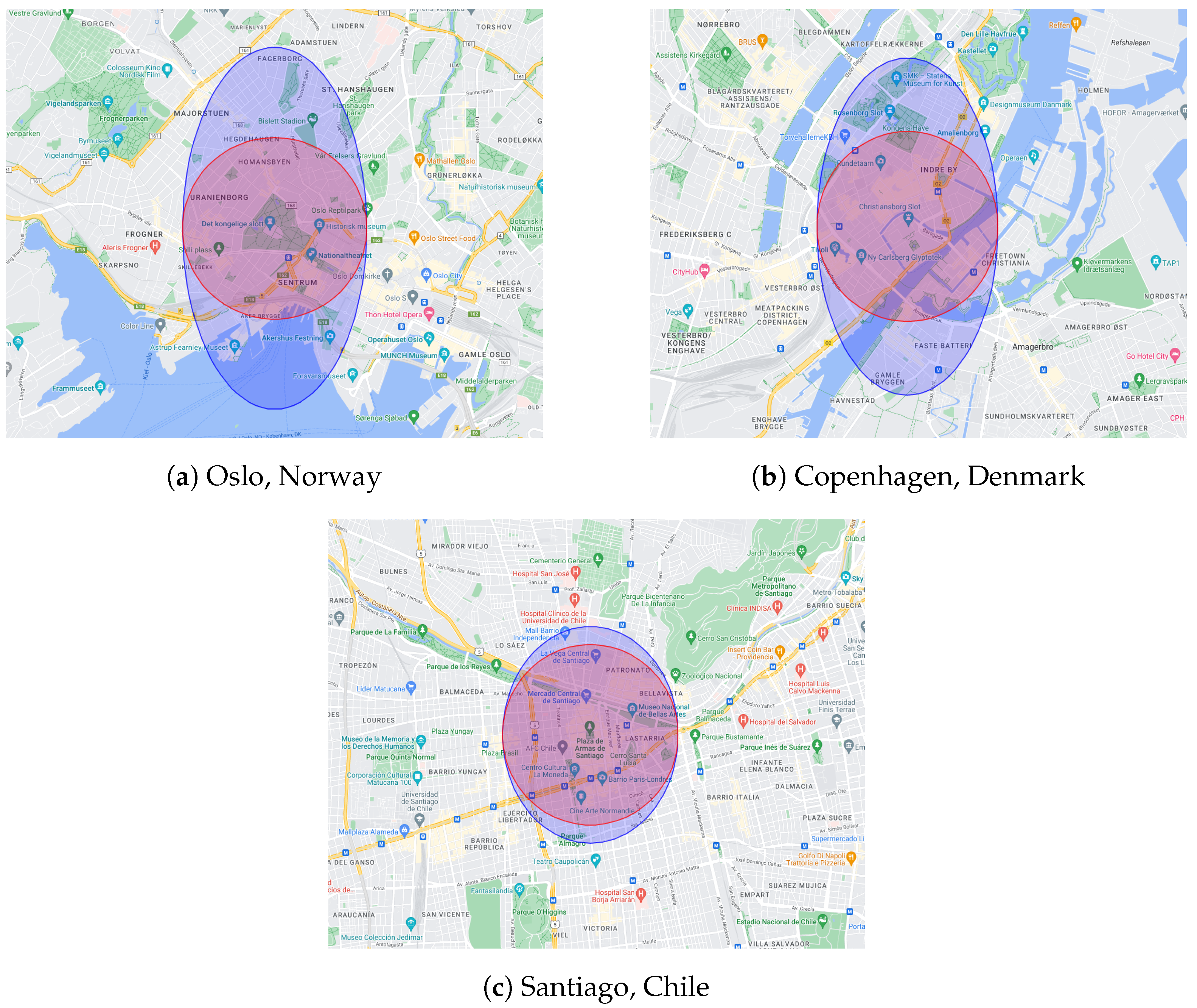
Figure 1 shows the area defined by the Euclidean and haversine distance metrics for three cities of the world, Oslo, Copenhagen, and Santiago. In each figure, the Euclidean distance area is colored blue, and all geographical points whose distance is less than 0.015 degrees are considered. For the haversine metric, a distance in meters is computed that is equal to 0.015 degrees for the horizontal axis (longitude). All points whose haversine distance is less than that distance are represented by the area in red.

As illustrated in the images, the area defined by the Euclidean distance is biased in its identification of the nearest neighbors: the points on the vertical axis (latitude) are closer in Euclidean distance than are the points at the same physical distance (in meters) on the horizontal axis. This bias prejudices the prediction of KNN since trips that have origins and destinations close to the trip to be estimated and that should be considered are discarded. Note that this bias depends on the geographic location of the city: cities closer to the earth’s poles have a larger bias. The KNN model that uses the haversine distance to determine the observation’s neighbors is denoted as “KNN-H”, while we define the standard Euclidean uniform KNN as “KNN-U”.

The KNN variant under consideration assigns different weights to neighbor observations based on their proximity to the point $\mathbf{x}$ being predicted. Those neighbors that are closer to the point have a higher weight than do those that are distant. Let $d(\mathbf{x},y_i)$ be the distance from a point $\mathbf{x}$ to one $y_i$, for i in the set of k-neighbors of $\mathbf{x}$, $N_k\left(\mathbf{x}\right)$. The predicted value $\widehat{t}$ corresponds to the following

$$\begin{array}{cccc} & \widehat{t}=\sum _{i\in N_k\left(\mathbf{x}\right)}{w}_i{t}_i,\hfill & \hfill & \end{array}$$

(6a)

$$\begin{array}{cccc} & w_i={\left(\sum _{j\in N_k\left(\mathbf{x}\right)}\frac{1}{d(\mathbf{x},y_j)}\right)}^{-1}\frac{1}{d(\mathbf{x},y_i)},\hfill & & i\in N_k\left(x\right).\hfill \end{array}$$

(6b)

This variant is known as weighted k-nearest neighbors (KNN-W) and as KNN-WH in the case where the haversine distance is used.

Nevertheless, the KNN-W does not take into account the bias that the predicted values may have due to the chosen observations. To illustrate this bias, we provide the following example. In Figure 2, we show two trips to be estimated, both represented with a red dashed line, and we also show the nearest O-D neighbors for these trips. In Figure 2a, the trip is shorter than the average distance traveled by its O-D neighbors, so KNN and KNN-W estimate a longer travel time than the trip actually has. In Figure 2b, the example trip covers a longer distance than the average of its O-D neighbors, so the travel time is underestimated. Moreover, in both cases, the time estimation of the trip is the same even though they should be significantly different.

For observations whose neighbors have travel distances smaller than or larger than the one we seek to estimate, we propose a correction mechanism, in which these values are adjusted based on the distances. Let ${\widehat{t}}^c$ be the travel-time-corrected estimation, let $t_i$ be the travel time of the trip $i\in N_k\left(\mathbf{x}\right)$, let $w_i$ be the weight determined by KNN-W, and let d be the distance of the trip to be predicted. Then, we obtain the following:

$${\widehat{t}}^c=\sum _{i\in N_k\left(\mathbf{x}\right)}\frac{d}{d_i}{w}_i{t}_i.$$

(7)

This new variant is referred to as KNN-$\overline{\mathrm{W}}$H, which means that it considers the weighted KNN, the haversine distance, and a correction factor applied exclusively to the weighted part.

4.2. Time Partitioning Predicting Methods

The time of day the trip occurs provides additional information that can be used to estimate travel times with higher accuracy. The KNN-W method requires that all the input features of the point to be predicted can be related through a distance metric, which is not necessarily the case for the travel time estimation problem (i.e., time of the day such as the afternoon versus morning). In general, for this type of problem, time intervals are determined where travel times are similar, and then estimations are made with KNN-W. These intervals are usually defined arbitrarily. In this section, a new method is described for incorporating the time-of-the-day dimension into KNN models.

The objective is to find a partition of the daytime (24 h) that groups more similar neighbors for the point to estimate. The aggregation of time points uses the time of the day when the trip started, and then its neighbors are defined according to this daytime. The partition of the time horizon consists of several disjoint time blocks that are usually arbitrarily defined. There are two challenges to be addressed for finding a partition: (1) how to determine the times of the day when one time block ends and the next begins and (2) how many blocks are considered in the partition. For the first challenge, we propose a method based on binary search that defines these time limits with high granularity. For the second, we determine the number of blocks as a hyperparameter to be defined based on the prediction errors in the test data set.

Let P be the number of blocks in the time partition, and let $[{\ell }_{1,i},{\ell }_{2,i})$ be the time interval associated with the partition $i=1,\dots ,P$. Let $D^{\prime }$ be the number of observations for model training. We seek to find a configuration of the time partition, such that the total MAPE is minimal:

$$\begin{array}{ccc} & \mathrm{MAPE}=\frac{1}{\left|D^{\prime }\right|}\sum _{p\in P}\sum _{\begin{array}{c}i\in \{1,\dots ,D^{\prime }\},\\ {\tau }_i\in [{\ell }_{1,p},{\ell }_{2,p})\end{array}}\frac{|t_i-{\widehat{t}}_i|}{max\{t_i,1\}},\hfill & \end{array}$$

(8a)

$$\begin{array}{cccc} & {\widehat{t}}_j=\sum _{\begin{array}{c}i\in N_k\left({\mathbf{x}}_{\mathbf{j}}\right),\\ {\tau }_i\in [{\ell }_{1,\overline{p}},{\ell }_{2,\overline{p}})\end{array}}\frac{d_j}{d_i}{w}_i{t}_i,\hfill & \hfill & \forall j\in \{1,\dots ,D^{\prime }\},\hfill \end{array}$$

(8b)

where $\overline{p}$ is such that the time ${\tau }_j$ of point $j\in \{1,\dots ,D^{\prime }\}$ to be predicted is in the time interval $[{\ell }_{1,\overline{p}},{\ell }_{2,\overline{p}})$.

The binary search of this method checks each time limit independently and modifies them as long as the prediction error is lower than the current one. For this purpose, it considers a training data set and a test data set. Consider two adjacent time blocks, block 1 and block 2, with block 1 preceding block 2. Let ${\ell }_1$ be the starting time of block 1 and ${\ell }_2$ be the ending time of block 2. This algorithm finds the end limit of block 1 $\ell \in [{\ell }_1,{\ell }_2]$ (and, therefore, the start limit of block 2). When the time limits are before and after midnight, daytime is considered to be continuous in that interval. That is, the time values are such that …23:58, 23:59, 00:00, 00:01, …, for hours of the day numbered from 0 to 23.

Let $m(t_1,t_2)$ be the average MAPE error (prediction error) for the test data set, with the training data for a block delimited between times $t_1$ and $t_2$ being used. Let $q(t_1,t_2)$ be the number of observations in the test data set for times $t_1$ and $t_2$. The binary search algorithm (BSA), for a time limit between two adjacent blocks, is described in Algorithm 1.    

Algorithm 1: Binary search algorithm.

Input:  Tolerance $\epsilon >0$, time points ${\ell }_1,{\ell }_2$  Output:  Value of time ℓ 1 $\ell \leftarrow ({\ell }_1+{\ell }_2)/2$; 2 compute $m_0=\frac{q({\ell }_1,\ell )}{q({\ell }_1,{\ell }_2)}m({\ell }_1,\ell )+\frac{q(\ell ,{\ell }_2)}{q({\ell }_1,{\ell }_2)}m(\ell ,{\ell }_2)$; 3 ${\ell }_1^{\prime }\leftarrow ({\ell }_1+\ell )/2$; 4 ${\ell }_2^{\prime }\leftarrow (\ell +{\ell }_2)/2$； 5 while ${\ell }_2^{\prime }-{\ell }_1^{\prime }>\epsilon$ do 6   compute $m_1=\frac{q({\ell }_1,{\ell }_1^{\prime })}{q({\ell }_1,{\ell }_2)}m({\ell }_1,{\ell }_1^{\prime })+\frac{q({\ell }_1^{\prime },{\ell }_2)}{q({\ell }_1,{\ell }_2)}m({\ell }_1^{\prime },{\ell }_2)$; 7   compute $m_2=\frac{q({\ell }_1,{\ell }_2^{\prime })}{q({\ell }_1,{\ell }_2)}m({\ell }_1,{\ell }_2^{\prime })+\frac{q({\ell }_2^{\prime },{\ell }_2)}{q({\ell }_1,{\ell }_2)}m({\ell }_2^{\prime },{\ell }_2)$; 8   set $m^{*}=min\{m_0,m_1,m_2\}$; 9   if $m_1=m^{*}$ then 10     ${\ell }_2^{\prime }\leftarrow ({\ell }_1^{\prime }+\ell )/2$; 11     $\ell \leftarrow {\ell }_1^{\prime }$; 12     ${\ell }_1^{\prime }\leftarrow ({\ell }_1+{\ell }_1^{\prime })/2$; 13   end 14   if $m_2=m^{*}$ then 15     ${\ell }_1^{\prime }\leftarrow (\ell +{\ell }_2^{\prime })/2$; 16     $\ell \leftarrow {\ell }_2^{\prime }$; 17     ${\ell }_2^{\prime }\leftarrow ({\ell }_2^{\prime }+{\ell }_2)/2$; 18   end 19   if $m_0=m^{*}$ then 20     ${\ell }_1^{\prime }\leftarrow ({\ell }_1^{\prime }+\ell )/2$; 21     ${\ell }_2^{\prime }\leftarrow (\ell +{\ell }_2^{\prime })/2$; 22   end 23 end 24 return ℓ

This algorithm receives as input a tolerance $\epsilon >0$, which represents the level of detail with which the time block limits are revised. Furthermore, this algorithm receives a reference time limit where block 1 begins, ${\ell }_1$, and a reference time where block 2 ends, ${\ell }_2$. The search starts with the time limit between these two blocks in the middle of the interval, with a MAPE error $m_0$ (i.e., the MAPE over all the test data for both intervals). The initial search time values ${\ell }_1^{\prime }$ and ${\ell }_2^{\prime }$ are also computed. As long as these search time values have a difference greater than $\epsilon$, the block time limits continue to be revised. The MAPE for each time limit alternative, ${\ell }_1^{\prime }$ and ${\ell }_2^{\prime }$, is computed, and then the option with the lowest MAPE is determined. Depending on which option is better, the values of ${\ell }_1^{\prime }$, ${\ell }_2^{\prime }$ and ℓ are updated accordingly. When the algorithm stops, the value of time ℓ is returned. Finally, considering that Algorithm 1 is an implementation of the well-known binary search algorithm, the time complexity of the algorithm is $O\left(\log n_t\right)$, where $n_t$ is the number of possible values between ${\ell }_1$ and ${\ell }_2$.

The algorithm for finding a time partition uses the previously described BSA. In this partition algorithm, each limit is revised using the binary search and updated until there are no more improvements in their prediction errors. The time partitioning algorithm (TPA) is detailed in Algorithm 2.    

Algorithm 2: Time partitioning algorithm.

Input:  Tolerance $\epsilon >0$, list of time points L  Output:  List of new time points L 1 set list $R=L$; 2 while $R\ne Ø$ do 3   get a time point $\ell \in R$; 4   remove ℓ from R and L; 5   set ${\ell }_1=max\{r\in L|r<\ell \}$; 6   set ${\ell }_2=min\{r\in L|r>\ell \}$; 7   ${\ell }^{\prime }=\mathrm{BSA}({\ell }_1,{\ell }_2)$; 8   if ${\ell }^{\prime }\ne \ell$ then 9     add ${\ell }_1$ and ${\ell }_2$ to R; 10   end 11   add ${\ell }^{\prime }$ to L; 12 end 13 return L

This algorithm receives as input a tolerance $\epsilon >0$ (input for the BSA) and an initial list of time limits L. This list is an initial time partition (it can be just a random set of values). The list R is a list of values to be revised and is initialized equal to L. As long as the list R is not empty, a value ℓ is randomly taken from the list R and then removed from both R and L. The time limits adjacent to ℓ, ${\ell }_1$ and ${\ell }_2$ are identified, which are then used for the BSA. The returned time is ${\ell }^{\prime }$, and if ${\ell }^{\prime }$ is different from ℓ, then ${\ell }_1$ and ${\ell }_2$ are added back to the list of values to be revised, R. The addition of ${\ell }_1$ and ${\ell }_2$ to R allows the algorithm to search over the limits of the neighbors, which could be modified due to the current adjustment. Finally, ${\ell }^{\prime }$ is added to L. The algorithm returns the list L of time limits for the blocks.

The time complexity for Algorithm 2 is $O(n_{k}log\left(n_t\right))$, where $n_t$ is the largest number of possible time options between two time points belonging to L, and $n_k$ is the number of iterations of the algorithm. In the best-case scenario, $n_k$ is equal to the length of list L. However, in the worst-case scenario, $n_k$ could be as large as all possible separations of the timeline.

Note that the weighted version of KNN (using Equation (6)) is denoted as KNN+, which uses the haversine distance, with the correction criterion (7) and that, for a given number of blocks, applies the TPA.

5. Computational Experiments

In this section, the computational results of the proposed KNN and the time partitioning algorithm (TPA) for the real O-D data are described . To compare the performance of our methods, we considered models and algorithms commonly used for regression analysis in machine learning. The experiments were organized so that our proposed improvements could be analyzed independently.

5.1. Dataset Description and Preprocessing

The data came from a taxi app called Fantaxico, which operates in Santiago, Chile. The company has a fleet of taxis that serve the entire city (covering an area of 641 km²). Each vehicle generates GPS data pulses every 15 s, recorded in the company’s database. The available data considered for our computational study contained the equivalent of 300 GB of GPS traces, collected in March (2014, 2015, 2016), July (2014, 2015, 2016), and November (2014, 2015). We chose these months because they do not have events that could have affected the nature of travel times (e.g., vacation periods, festivities, etc.).

For these months, the dataset included 630,823 different origin–destination pairs (O-D pairs), but after the cleaning process, we obtained a total of 356,930 O-D pairs. We first removed the trips outside Santiago and all the origins or destinations outside the following coordinates: latitude −33.87 to −33.15 and longitude −70.98 to −70.40. This process removed a total of 14,193 trips, reducing the total number to 616,310. Then, we eliminated all the trips that were less than 30 m and more than 80 km long, removing 164,184 trips. We also excluded weekend trips, given that our focus is to model blocks of time based on weekdays. This process eliminated 56,028 trips, leaving 396,138 data points. The last 39,208 removed data points corresponded to trips with less than 30 s of duration or more than 3 h of duration or those with an average speed less than 2 km per hour (kph) or higher than 110 kph. In summary, our final dataset consisted of 356,930 trips and seven variables: latitude and longitude for the origin and destination, the length of the trip, the time of the trip, and the duration of the trip (the variable to predict).

In each experiment, the data were split into blocks, and k-fold cross-validation was applied to estimate the MAPE of the model. k-fold cross-validation is a method to estimate the performance of the model that partitions the original data into k-different folds. For each k-1 fold combinations, the model is trained using the data, and the remaining fold is used for testing, obtaining one training and one testing performance observation. This process is repeated k-times using each of the k-folds as test data, generating k-different evaluations, from which the mean and standard deviation are computed. For the assessment of performance in each experiment, the MAPE and their corresponding standard deviations are reported.

5.2. Initial Model Comparison

In the initial experiment, standard KNN algorithms with uniform and weighted predictions were studied, along with other popular baseline models such as regression trees and gradient boosting with regression trees. Additionally, an extra regression tree model was considered, incorporating the starting time of the trip as a variable, denoted as RT-Time. The KNN-based models outlined in Section 4 were as follows:

• KNN-U: KNN with Euclidean distance using uniform prediction.
• KNN-W: KNN with Euclidean distance using weighted prediction.
• KNN-WH: KNN with haversine distance using the weighted prediction.
• KNN-$\overline{\mathbf{W}}$H: KNN-WH with the bias correction in (7).
• KNN+: KNN-$\overline{\mathrm{W}}$H that applies the TPA for a given number of blocks (used in experiments 5.3 and 5.4).

For each model, the best hyperparameters were searched to check that the final models were not overfitted. The final hyperparameter k was 20 neighbors for all KNN-based models and depths of 8, 8, and 12 for the regression tree, gradient boosting, and RT-Time, respectively. We also chose 100 trees for gradient boosting. Given the computational effort needed for some models, in this initial experiment, dataset was limited to 90,000 O-D data points.

The aggregated results are shown in

Table 2. Average training and test results (mean and standard deviation) for baseline models with over 90,000 data points.

Model	Hyperparameters	Training Error	Testing Error
G-Boosting	depth $=8$, trees $=100$	44.52 (0.36)	48.10 (1.12)
KNN-U	$k=20$	39.78 (0.01)	41.87 (0.71)
KNN-W	$k=20$	0.00	39.44 (0.66)
KNN-WH	$k=20$	0.00	39.37 (0.70)
KNN-$\overline{\mathrm{W}}$H	$k=20$	0.00	37.93 (0.42)
Regression Tree	depth $=8$	59.95 (0.30)	60.70 (1.57)
RT-Time	depth $=12$	46.22 (0.29)	51.12 (1.64)

. First, it can be observed that the models were not overfitted since similar MAPEs were obtained for training and testing. The exceptions are the KNN with weighted prediction, with an actual training error of 0.0. This can explained by the fact that in the training process, the closest neighbor of a data point is the same point, obtaining infinite importance in the final prediction. Both KNN baseline models (KNN-U and KNN-W) showed the lowest testing error among classical baselines, with a significant difference with respect to decision trees and gradient boosting. Even though we gave an additional variable to RT-Time, it could not overcome the KNN models. Standard KNN models were better than were tree-based models, and KNN-WH and KNN-$\overline{\mathrm{W}}$H were the best models. Although KNN-WH was not significantly better than was KNN-W (t-test hypothesis testing, p-value of 0.875), this method uses the haversine distance (the correct metric to measure the distance of geographical positions). Finally, KNN-$\overline{\mathrm{W}}$H was significantly better than all the other models according to the t-test hypothesis testing and obtained a p-value of 0.004 and 0.003 with respect to its two closest models KNN-WH and KNN-W.

5.3. Fixed Time Partition

This section outlines the investigation into how the time of day when a trip starts affects its duration. We adopt a fixed time partition of the day to differentiate between times of heavy traffic congestion and lighter traffic periods. This partition allowed us to categorize trips made under similar circumstances (congestion), enabling control over these external factors This initial time partition was taken from the division made by the Santiago subway for fare pricing. This fare reflects the movement of people during the work week, which we believe is related to traffic congestion in the city. The time blocks defined by the subway are as follows:

• 7:01 to 9:00, high fare.
• 9:01 to 18:00, medium fare.
• 18:01 to 20:00, high fare.
• 20:01 to 20:45, medium fare.
• 20:46 to 23:00, low fare.
• 23:00 to 6:00, closed.
• 6:01 to 7:00, low fare.

As in the initial experiments, we considered KNN models (all their variants) and tree-based models. RT-Time considers the starting time of the trip as a variable, but we still ran it for each time block. Similarly to before, we searched for the best hyperparameters, checking that the final models were not overfitted. The final hyperparameters were 20 neighbors for KNN-based models and depths of 8, 12, and 4 for the regression tree, RT-Time, and gradient boosting, respectively. We also chose 60 trees for gradient boosting.

Table 3. Test results (mean and standard deviation) for the prediction models per time block (Best results in bold).

	G-Boosting	KNN-U	KNN-W	KNN-WH	KNN-$\overline{\mathbf{W}}$H	Regression Tree	RT-Time
Block 0	36.36 (2.21)	25.54 (1.13)	23.53 (1.09)	23.20 (1.05)	21.13 (0.64)	37.55 (2.05)	35.67 (2.13)
Block 1	60.29 (2.66)	40.41 (0.72)	38.60 (0.70)	38.37 (0.72)	36.78 (0.49)	61.55 (1.40)	54.31 (0.62)
Block 2	65.01 (2.68)	47.23 (1.37)	45.35 (1.27)	45.07 (1.30)	42.25 (0.94)	67.06 (3.24)	61.47 (3.64)
Block 3	61.52 (3.02)	44.56 (1.25)	42.79 (1.33)	42.73 (1.27)	38.99 (0.76)	60.39 (2.47)	52.53 (2.68)
Block 4	57.96 (3.79)	40.97 (1.01)	39.31 (0.98)	39.34 (1.03)	35.37 (0.52)	55.96 (2.08)	47.53 (2.02)
Block 5	43.49 (2.62)	31.07 (0.57)	28.86 (0.50)	28.85 (0.51)	26.86 (0.28)	44.54 (1.29)	41.35 (1.00)
Block 6	41.12 (3.55)	34.00 (3.04)	30.97 (3.27)	31.37 (4.48)	25.05 (2.51)	45.49 (3.49)	43.36 (5.32)
Average	54.52	37.87	35.95	35.80	33.58	55.40	49.60

shows the test results for the prediction models for each block of the partition. We computed the average and standard deviation of the errors for each block. At the bottom of the table is the average of the errors for all blocks. Training errors are omitted, but all errors appear similar to test errors except for those of the weighted KNN models: they obtained a training error of 0.0 because of the infinite importance of the same data point.

As observed previously, the KNN-based methods showed the best results, with significant differences with respect to the tree-based models. The performance of RT-Time was worse than that of the KNN models despite it having an additional variable (the time at which the trip began) as input. However, this variable dud help to improve the performance of this method over the other tree-based models, gradient boosting, and regression trees. These results also show that KNN-$\overline{\mathrm{W}}$H had the lowest test errors for all time blocks, with significant differences. Specifically, the average MAPE of KNN-$\overline{\mathrm{W}}$H was 33.39. We also ran KNN+, obtaining an even lower average performance of 32.96; however, since this method changes the time blocks, rendering them incomparable to the original ones, we have not included the KNN+ results in Table 3. KNN-U was the KNN variant with the worst performance, showing that the changes included in KNN-W and KNN-WH generate improvements in the predictions. The performance was similar with respect to distance (Euclidean or haversine), and the differences between KNN with the weighted prediction (KNN-W), against the same version but with a change in the distance to haversine (KNN-WH), were minimal, with MAPEs of 37.48 and 37.35, respectively.

A t-test hypothesis test was used to analyze whether the mean MAPEs among the models were statistically different. In all cases, the results of the KNN variants were statistically better compared to those of the tree-based models, and the differences were statically significant at the level of $0.01$. In the comparison of the KNN models, KNN-W was statistically significantly better than the KNN-U prediction in six of the seven blocks (block 6 had a p-value of 0.046). We also applied a t-test among all blocks (one test per block), and there were no statistically significant differences between the average values when the haversine distance was used. However, when the results of the KNN variants were compared with those of KNN-$\overline{\mathrm{W}}$H, in all cases, our proposed method obtained the lowest MAPE, with differences that were statistically significant at the $0.01$ level.

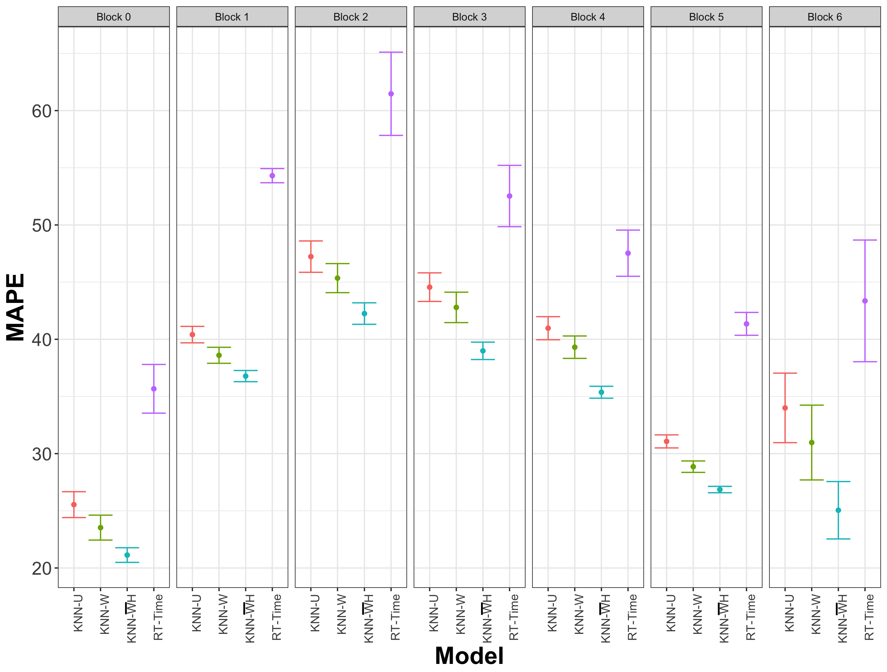
The training and test results are shown in Figure 3 for models KNN-$\overline{\mathrm{W}}$H, KNN-U, KNN-W, and RT-Time. The overlap of the training and test model MAPEs indicates that the models were not overfitted. It can also be observed that KNN-W was slightly better than KNN-U. The model KNN-$\overline{\mathrm{W}}$H significantly outperformed all models, with statistically significant differences: in six of the seven blocks, the standard deviations did not overlap between them. Even in the last block, when the standard deviation almost overlapped, the t-test returned a p-value of 0.00026 (for the closest average), indicating a statistically significant difference.

5.4. Variable Time Partition

This subsection describes the analysis of the effect of the time partition algorithm on MAPE and the final blocks using random samples of 90,000 data points. The analysis consisted of first comparing the performance of KNN+ (using TPA) against KNN-$\overline{\mathrm{W}}$H with fixed and uniform time partitions, with different numbers of blocks being considered. We then analyzed the time blocks obtained for KNN+ to inform management guidance to urban passenger transport operators on how these time blocks might impact their business.

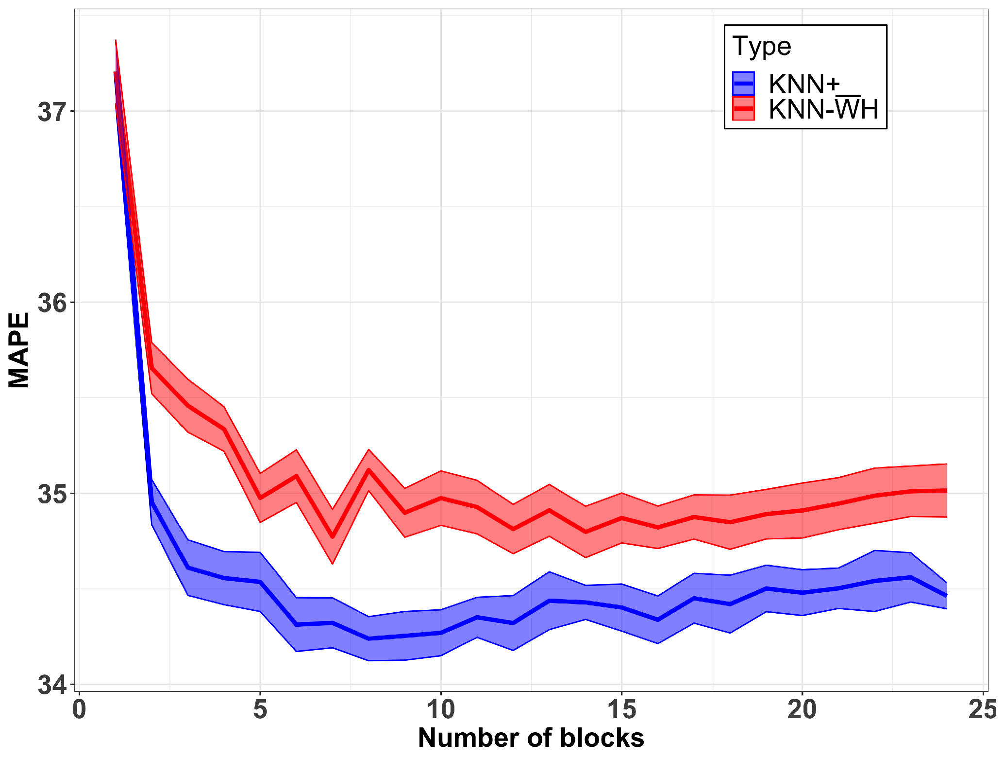
In the experiment, the MAPE of the model using 10-fold cross-validation for different numbers of blocks was estimated. The results are shown in Figure 4. Two curves were plotted, one for the KNN+ model and the other for the KNN-$\overline{\mathrm{W}}$H with fixed time blocks, and in both cases, the average MAPE and an interval of one standard deviation were considered (average plus/minus one standard deviation). Equidistant blocks were considered as input blocks for the models. As expected, both models had the same results for a single block. When the number of blocks increased, the MAPE decreased in both cases up to 10 blocks and then remained stable. It can observed that both models were able to avoid overfitting by the number of blocks. We can also observe that the KNN+ MAPE was significantly lower than the KNN-$\overline{\mathrm{W}}$H MAPE for any number of blocks greater than 1 (p-value less than 0.01). We cab conclude that KNN+ can successfully make use of the starting time of the trip to improve the performance.

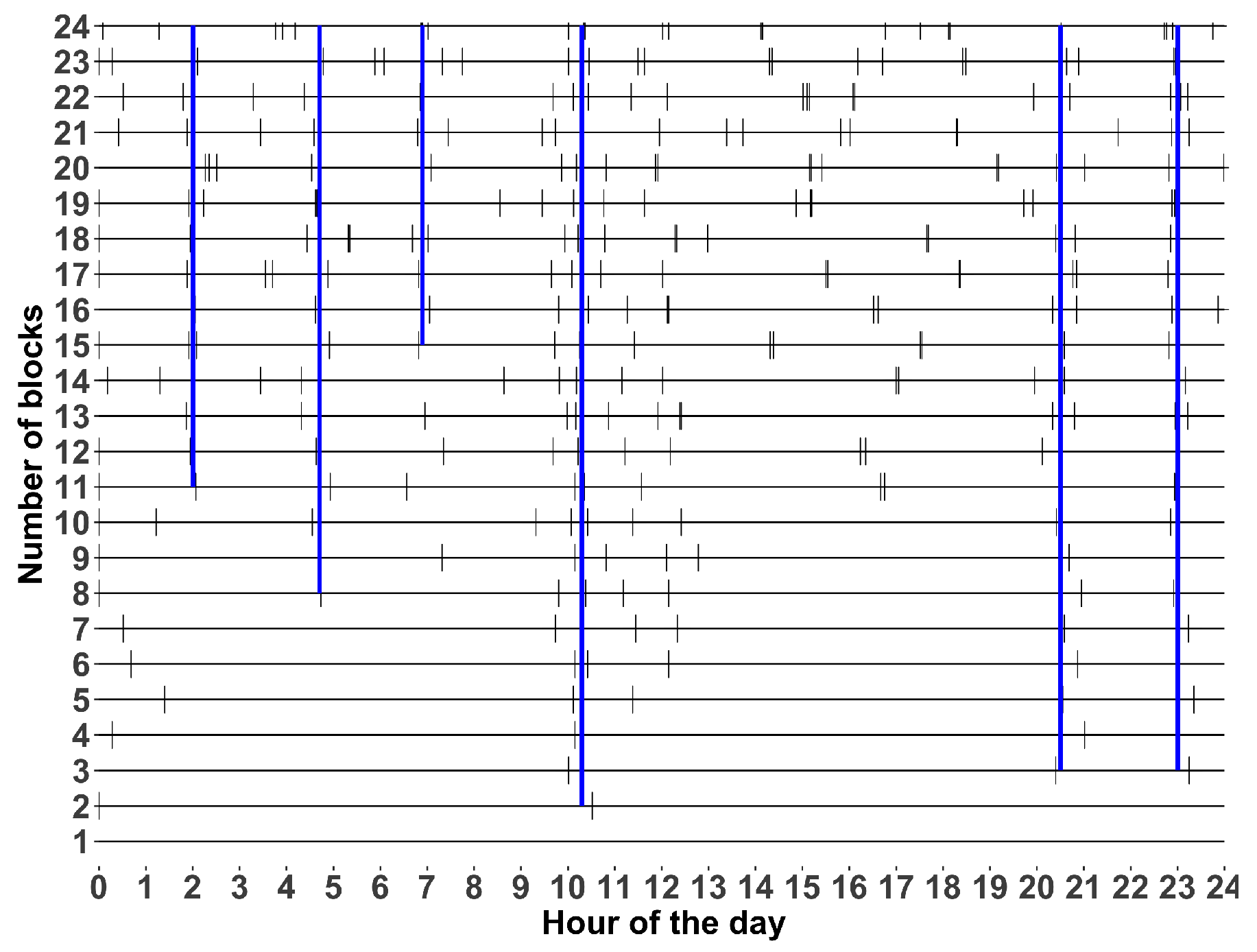
Given the better performance of our proposed KNN+ model, we analyzed the generated blocks for this model. In this case, we considered a single iteration of the 10-fold cross-validation and plotted the different blocks obtained by KNN+. The results can be observed in Figure 5, where the X-axis corresponds to 24 h of the day, and the Y-axis corresponds to the number of blocks. The vertical black dashed lines correspond to the separation produced by the model. To facilitate visualization of the plot, we included blue lines corresponding to the most common hour separation obtained by the model.

The figure shows six time slots (blocks): 2:00–4:30, 4:30–7:00, 7:00–10:00, 10:00–20:00, 20:00–23:00, and 23:00–2:00. As observed, the time blocks are different from the original seven time blocks taken from the Metro and Public Transportation System (Santiago’s subway). This has some implications for both taxi operators and planners. For the former, since taxis do not have the same behavior as that of public transportation users, taxi fares can be determined according to the proposed blocks. In addition, taxi operators and drivers can be better informed and reduce uncertainty and reduced their chances of staying in traffic bottlenecks and gridlock by improving decisions about departure times or routes. For the latter, the procedure can provide time blocks that give a more detailed understanding of how congestion builds up and dissipates over time, as a prediction of a faster adaptation to the changing conditions of traffic. This adaptability can help to prevent congestion from worsening and can alleviate it more effectively, for instance, by dynamically adjusting traffic signals or toll rates.

6. Conclusions

This study investigated the origin–destination (O-D) travel time estimation problem, aiming to predict the duration of a trip based on the origin and destination locations, along with the time of day. We propose enhancements to the KNN model, targeting two key limitations: the bias inherent in handling such data and the challenge of integrating a new input dimension (travel starting time) into the prediction process. This paper proposes new mechanisms and algorithms to handle these challenges that significantly improve O-D travel time estimation. The models consider the haversine distance instead of the Euclidean distance, improving the distance computation among trips. Moreover, the new models estimate the distance of a trip based not only on the time of their k closest neighbors but also include the distance from neighboring trips. The proposed combination demonstrated statistically significant improvements compared to current state-of-the-art models in a large taxi trip data set from Santiago, Chile.

The KNN+ model also incorporates a heuristic (TBA) to adaptively search for the best time block partition. That is, instead of using predefined time blocks as is done in the recently proposed methods in the literature, the heuristic includes a binary search over the length of a day, finding time blocks that improve the estimation of the travel time. The proposed algorithm has advantages compared to the model with a predefined time partition, achieving a superior performance to all models. To do this, our model incorporates an additional input variable (time) that allows us to partition the neighbor search. This algorithm, which is new in the literature, could be studied for other predictive problems and contexts related to machine learning. To extend this method, how the inclusion of other variables, such as the day of the week, the month of the year, or the weather of the city, impacts the prediction of time can be studied.

In the experiments conducted, time slots defined by the public transportation agency and the metro system (subway) were utilized, revealing their inapplicability to the taxi data at hand. An adaptive model capable of handling traffic conditions, particularly in travel times, can significantly enhance the development of more effective traffic management decisions and planning policies. Additionally, for taxi operators, such a model can enhance their situational awareness, mitigate uncertainty, assist in identifying optimal routes, and optimize pricing strategies.

References

- Bertsimas, D.; Delarue, A.; Jaillet, P.; Martin, S. Travel time estimation in the age of big data. Oper. Res. 2019, 67, 498–515. [Google Scholar] [CrossRef]
- Wu, X.; Kumar, V.; Ross Quinlan, J.; Ghosh, J.; Yang, Q.; Motoda, H.; McLachlan, G.J.; Ng, A.; Liu, B.; Yu, P.S.; et al. Top 10 algorithms in data mining. Knowl. Inf. Syst. 2008, 14, 1–37. [Google Scholar] [CrossRef]
- Vlahogianni, E.I.; Karlaftis, M.G.; Golias, J.C. Short-term traffic forecasting: Where we are and where we’re going. Transp. Res. Part C Emerg. Technol. 2014, 43, 3–19. [Google Scholar] [CrossRef]
- Woodard, D.; Nogin, G.; Koch, P.; Racz, D.; Goldszmidt, M.; Horvitz, E. Predicting travel time reliability using mobile phone GPS data. Transp. Res. Part C Emerg. Technol. 2017, 75, 30–44. [Google Scholar] [CrossRef]
- Prokhorchuk, A.; Dauwels, J.; Jaillet, P. Estimating Travel Time Distributions by Bayesian Network Inference. IEEE Trans. Intell. Transp. Syst. 2020, 21, 1867–1876. [Google Scholar] [CrossRef]
- Putatunda, S.; Laha, A. Travel Time Prediction in Real time for GPS Taxi Data Streams and its Applications to Travel Safety. Hum. Cent. Intell. Syst. 2023, 3, 381–401. [Google Scholar] [CrossRef]
- Satrinia, D.; Saptawati, G.P. Traffic speed prediction from GPS data of taxi trip using support vector regression. In Proceedings of the International Conference on Data and Software Engineering (ICoDSE), Palembang, Indonesia, 1–2 November 2017; pp. 1–6. [Google Scholar] [CrossRef]
- Gmira, M.; Gendreau, M.; Lodi, A.; Potvin, J.Y. Travel speed prediction based on learning methods for home delivery. EURO J. Transp. Logist. 2020, 9, 100006. [Google Scholar] [CrossRef]
- Sun, S.; Chen, J.; Sun, J. Traffic congestion prediction based on GPS trajectory data. Int. J. Distrib. Sens. Netw. 2019, 15, 1550147719847440. [Google Scholar] [CrossRef]
- Stipancic, J.; Miranda-Moreno, L.; Labbe, A.; Saunier, N. Measuring and visualizing space–time congestion patterns in an urban road network using large-scale smartphone-collected GPS data. Transp. Lett. 2019, 11, 391–401. [Google Scholar] [CrossRef]
- Zheng, L.; Xia, D.; Zhao, X.; Tan, L.; Li, H.; Chen, L.; Liu, W. Spatial–temporal travel pattern mining using massive taxi trajectory data. Phys. A Stat. Mech. Its Appl. 2018, 501, 24–41. [Google Scholar] [CrossRef]
- Krause, C.M.; Zhang, L. Short-term travel behavior prediction with GPS, land use, and point of interest data. Transp. Res. Part B Methodol. 2019, 123, 349–361. [Google Scholar] [CrossRef]
- Chughtai, J.U.R.; Haq, I.U.; Shafiq, O.; Muneeb, M. Travel Time Prediction Using Hybridized Deep Feature Space and Machine Learning Based Heterogeneous Ensemble. IEEE Access 2022, 10, 98127–98139. [Google Scholar] [CrossRef]
- Vankdoth, S.R.; Arock, M. Deep intelligent transportation system for travel time estimation on spatio-temporal data. Neural Comput. Appl. 2023, 35, 19117–19129. [Google Scholar] [CrossRef]
- Sheng, Z.; Lv, Z.; Li, J.; Xu, Z. Deep spatial-temporal travel time prediction model based on trajectory feature. Comput. Electr. Eng. 2023, 110, 108868. [Google Scholar] [CrossRef]
- Zhuang, L.; Wu, X.; Chow, A.H.; Ma, W.; Lam, W.H.; Wong, S.C. Reliability-based journey time prediction via two-stream deep learning with multi-source data. J. Intell. Transp. Syst. 2024, 1–19. [Google Scholar] [CrossRef]
- Zhang, H.; Zhao, F.; Wang, C.; Luo, H.; Xiong, H.; Fang, Y. Knowledge Distillation for Travel Time Estimation. IEEE Trans. Intell. Transp. Syst. 2024, in press. [CrossRef]
- Zhou, X.; Yang, Z.; Zhang, W.; Tian, X.; Bing, Q. Urban Link Travel Time Estimation Based on Low Frequency Probe Vehicle Data. Discret. Dyn. Nat. Soc. 2016, 2016, 7348705. [Google Scholar] [CrossRef]
- Vu, L.H.; Passow, B.N.; Paluszczyszyn, D.; Deka, L.; Goodyer, E. Estimation of Travel Times for Minor Roads in Urban Areas Using Sparse Travel Time Data. IEEE Intell. Transp. Syst. Mag. 2021, 13, 220–233. [Google Scholar] [CrossRef]
- Sanaullah, I.; Quddus, M.; Enoch, M. Developing travel time estimation methods using sparse GPS data. J. Intell. Transp. Syst. Technol. Plan. Oper. 2016, 20, 532–544. [Google Scholar] [CrossRef]
- Ghandeharioun, Z.; Kouvelas, A. Link Travel Time Estimation for Arterial Networks Based on Sparse GPS Data and Considering Progressive Correlations. IEEE Open J. Intell. Transp. Syst. 2022, 3, 679–694. [Google Scholar] [CrossRef]
- Zhan, X.; Hasan, S.; Ukkusuri, S.V.; Kamga, C. Urban link travel time estimation using large-scale taxi data with partial information. Transp. Res. Part C Emerg. Technol. 2013, 33, 37–49. [Google Scholar] [CrossRef]
- NYCTLC. Trip Record Data. 2016. Available online: https://www.nyc.gov/site/tlc/about/tlc-trip-record-data.page (accessed on 25 March 2024).
- Zhan, X.; Ukkusuri, S.V.; Yang, C. A Bayesian mixture model for short-term average link travel time estimation using large-scale limited information trip-based data. Autom. Constr. 2016, 72, 237–246. [Google Scholar] [CrossRef]
- Wang, H.; Tang, X.; Kuo, Y.H.; Kifer, D.; Li, Z. A Simple Baseline for Travel Time Estimation using Large-scale Trip Data. ACM Trans. Intell. Syst. Technol. 2019, 10, 1–22. [Google Scholar] [CrossRef]
- Araujo, A.C.D.; Etemad, A. Deep Neural Networks for Predicting Vehicle Travel Times. In Proceedings of the IEEE Sensors, Montreal, QC, Canada, 27–30 October 2019; pp. 1–4. [Google Scholar] [CrossRef]
- Bishop, C.M.; Nasrabadi, N.M. Pattern Recognition and Machine Learning; Springer: Cham, Switzerland, 2006; Volume 4. [Google Scholar]
- Hastie, T.; Tibshirani, R.; Friedman, J.H.; Friedman, J.H. The Elements of Statistical Learning: Data Mining, Inference, and Prediction; Springer: Cham, Switzerland, 2009; Volume 2. [Google Scholar]
- Murphy, K.P. Machine Learning: A Probabilistic Perspective; MIT Press: Cambridge, MA, USA, 2012. [Google Scholar]
- Cover, T.; Hart, P. Nearest neighbor pattern classification. IEEE Trans. Inf. Theory 1967, 13, 21–27. [Google Scholar] [CrossRef]
- Wang, H. Nearest neighbors by neighborhood counting. IEEE Trans. Pattern Anal. Mach. Intell. 2006, 28, 942–953. [Google Scholar] [CrossRef] [PubMed]
- Ooi, H.L.; Ng, S.C.; Lim, E. Ano detection with k-nearest neighbor using minkowski distance. Int. J. Signal Process. Syst. 2013, 1, 208–211. [Google Scholar] [CrossRef]
- Bailey, T.; Jain, A. A Note on Distance-Weighted k-Nearest Neighbor Rules. IEEE Trans. Syst. Man Cybern. 1978, 8, 311–313. [Google Scholar] [CrossRef]
- Yao, Z.; Ruzzo, W.L. A regression-based K nearest neighbor algorithm for gene function prediction from heterogeneous data. BMC Bioinform. 2006, 7, 1–11. [Google Scholar] [CrossRef] [PubMed]
- Navot, A.; Shpigelman, L.; Tishby, N.; Vaadia, E. Nearest neighbor based feature selection for regression and its application to neural activity. Adv. Neural Inf. Process. Syst. 2005, 18. [Google Scholar]
- Liu, T.; Moore, A.W.; Gray, A. New Algorithms for Efficient High-Dimensional Nonparametric Classification. J. Mach. Learn. Res. 2006, 7, 1135–1158. [Google Scholar]
- Qin, W.; Zhang, M.; Li, W.; Liang, Y. Spatiotemporal K-Nearest Neighbors Algorithm and Bayesian Approach for Estimating Urban Link Travel Time Distribution From Sparse GPS Trajectories. IEEE Intell. Transp. Syst. Mag. 2023, 15, 152–176. [Google Scholar] [CrossRef]
Figure 1.
Area defined for the Euclidean (blue) and the haversine (red) distance for three different cities.
Figure 2.
KNN bias examples. The O-D travel time to be estimated is represented by a red dashed line, and the O-D neighbors are represented with blue dots.
Figure 3.
Results for KNN-H, KNN-U, KNN-W, and RT-Time. Each column subplot shows a block of time, with the corresponding average errors of the test results, while the lines represent one standard deviation.
Figure 4.
Average test results for KNN+ and KNN-H starting with equidistant numbers of blocks.
Figure 5.
Separation (dashed lines) of the hour of the day and most common hour separation (blue lines) based on the number of blocks. The X-axis shows the time of the day, while the Y-axis shows the number of blocks used.