Locally Exact Integrators for the Duffing Equation

Abstract

A numerical scheme is said to be locally exact if after linearization (around any point) it becomes exact. In this paper, we begin with a short review on exact and locally exact integrators for ordinary differential equations. Then, we extend our approach on equations represented in the so called linear gradient form, including dissipative systems. Finally, we apply this approach to the Duffing equation with a linear damping and without external forcing. The locally exact modification of the discrete gradient scheme preserves the monotonicity of the Lyapunov function of the discretized equation and is shown to be very accurate.

1. Introduction

Locally exact integrators are characterized by the property that they become exact for the linearization of the considered system around any point [1,2]. Thus we combine two well known procedures. First, nonlinear systems can be approximated by linear equations. Second, the exact discretization in an explicit form exists for any linear ordinary differential equation (ODE) with constant coefficients [3], see also Reference [4,5]. Locally exact schemes are linearly stable, A-stable and, in general, very accurate for trajectories in the vicinity of stable equlibria [2]. This class of numerical schemes has some similarity to Gautschi-type methods [6,7], Mickens’ approach [5] and exponential integrators [8,9]. However, to the best of our knowledge, most integrators produced within our approach are new, especially when modifications of the discrete gradient method are concerned [1,10], including the simplest (linearization-preserving [11]) modification in the case of the simple pendulum [12]. In general, our approach is especially effective for discrete gradient schemes. In the case of Hamiltonian systems discrete gradient schemes preserve the energy integral exactly, up to rounding errors [13,14]. We have shown that it is possible to keep this property while modifying discrete gradient schemes in a locally exact way [1,10].

In this paper we apply our approach to the systems which can be written in the so-called linear gradient form, see Reference [14], including dissipative systems. The discrete gradient method for this case is well known [14]. In Section 4 we construct its locally exact modification. However, one has to remember that, in general, a locally exact modification can spoil geometric properties of the original algorithm (and preservation of geometric properties of by numerical algorithms is of considerable advantage [6,15]). The geometric properties of the modified scheme should be studied separately.

The paper is divided into two parts. In Section 2 and Section 3 we present a short review on exact and locally exact integrators. In the second part, we discuss in more detail a particular case of the Duffing equation with a linear damping and without external forcing: $\ddot{x}+a\dot{x}-x+x^3=0$. We construct and test two locally exact discretizations of the Duffing equation. In Section 5 we show that the obtained locally exact modification of the discrete gradient method preserves a geometric property of the Duffing equation: monotonicity of the Lyapunov function.

2. Exact Integrators for Linear ODEs with Constant Coefficients

Let $\mathit{x}(t)$ be the general solution of an ordinary differential equation (ODE) with the initial condition $\mathit{x}(t_0)={\mathit{x}}_0$. The difference equation, satisfied by ${\mathit{x}}_n$, is called the exact discretization of this ODE if ${\mathit{x}}_n=\mathit{x}(t_n)$.

The exponential growth can serve as an elementary example. The equation ${\displaystyle \dot{x}=ax}$, $x(0)=x_0$, is satisfied by $x(t)=x_0{e}^{at}$. Therefore, we can define ${\displaystyle x_n:=x(nh)=e^{ahn}{x}_0}$, and this sequence obviously satisfies the difference equation $x_{n+1}=e^{ah}{x}_n$. Therefore, the geometric series with the common ratio $e^{ah}$ is the exact discretization of the linear equation ${\displaystyle \dot{x}=ax}$.

Exact discretization for the classical harmonic oscillator $\ddot{x}+{\omega }^{2}x=0$, $p=\dot{x}$, is less obvious but can be easily derived (see, e.g., Reference [16]):

$${\displaystyle x_{n+1}-2cos(\omega h)x_n+x_{n-1}=0,p_n=\frac{x_{n+1}-cos(\omega h)x_n}{\frac{sin(\omega h)}{\omega }}.}$$

(1)

However, in this case it is better to use the (equivalent) matrix form, which is more straightforward:

$$\left(\begin{array}{c}\omega x_{n+1}\\ p_{n+1}\end{array}\right)=\left(\begin{array}{cc}cos(\omega h)& sin(\omega h)\\ -sin(\omega h)& cos(\omega h)\end{array}\right)\left(\begin{array}{c}\omega x_n\\ p_n\end{array}\right).$$

(2)

It is interesting that in both above cases exact discretizations can be treated as deformations of the simplest numerical schemes. If $x_{n+1}=e^{ah}{x}_n$, then:

$$\frac{x_{n+1}-x_n}{{\delta }_1(h)}=a{x}_n,{\delta }_1(h):=\frac{e^{ah}-1}{a},{\delta }_1(h)\approx h\mathrm{for}h\to 0.$$

(3)

Similarly, Equations (1) are equivalent to

$$\frac{x_{n+1}-2x_n+x_{n-1}}{{({\delta }_2(h))}^2}+{\omega }^2{x}_n=0,p_n=\frac{x_{n+1}-x_{n-1}}{{\delta }_2(2h)},{\delta }_2(h)=\frac{2}{\omega }sin\frac{\omega h}{2},$$

(4)

where ${\delta }_2(h)\approx h$ for $h\to 0$. The above concise expression for $p_n$ was overlooked in Reference [16].

These examples can be generalized to all linear ODEs with constant coefficients, see [3]. Indeed, any linear ordinary differential equation, represented in a matrix form as

$$\frac{d\mathit{x}}{dt}=A\mathit{x}+\mathit{b},$$

(5)

(where $\mathit{x}=\mathit{x}(t)\in {\mathbb{R}}^d$, A is an invertible $d\times d$ matrix with constant real coefficients and $\mathit{b}=\mathrm{const}\in {\mathbb{R}}^d$) admits the following exact discretization (see Reference [17], Th. 3.1):

$${\mathit{x}}_{n+1}-{\mathit{x}}_n=A^{-1}(e^{h_{n}A}-I)\left(A{\mathit{x}}_n+\mathit{b}\right),$$

(6)

where $h_n=t_{n+1}-t_n$ and I is the unit matrix. Actually, the invertibility of A is not necessary. It is better to use the function ${\phi }_1$ (see, e.g., Reference [18])

$${\phi }_1(x)=\frac{e^x-1}{x}\mathrm{for}x\ne 0,{\phi }_1(0)=1,$$

(7)

which is analytic also at $x=0$. Therefore, the exact discretization of (5) can be expressed as

$${\mathit{x}}_{n+1}-{\mathit{x}}_n=h_n{\phi }_1(h_{n}A)\left(A{\mathit{x}}_n+\mathit{b}\right),$$

(8)

for any constant matrix A and constant vector $\mathit{b}$. Throughout this paper we will frequently use the function ${\phi }_1$ and similarly defined function

$${\displaystyle \mathrm{tanhc}(x)=\frac{tanh(x)}{x}\mathrm{for}x\ne 0,\mathrm{tanhc}(0)=1.}$$

(9)

Both functions are analytic in the neighbourhood of $x=0$.

3. Locally Exact Numerical Schemes

Exact discretizations can be used directly (e.g., in numerical integration of the Kepler problem [19], wave equation [20] and Schrödinger equation [21]) but this area of their application is rather limited. Here we present a more general approach in which exact integrators are used to modify and improve numerical schemes [2,17].

Definition 1.

A numerical scheme ${\mathit{x}}_{n+1}=\Phi ({\mathit{x}}_n,h_n)$ for an autonomous ODE $\dot{\mathit{x}}=F(\mathit{x})$ is locally exact if there exists a sequence ${\overline{\mathit{x}}}_n$ such that ${\overline{\mathit{x}}}_n-{\mathit{x}}_n=O(h_n)$ and the linearization of this scheme around ${\overline{\mathit{x}}}_n$ is identical with the exact discretization of the considered ODE linearized around ${\overline{\mathit{x}}}_n$ (for any n).

As far as the sequence ${\overline{\mathit{x}}}_n$ is considered, we often supress the index n and usually we confine ourselves to three special cases. The simplest case (small oscillations) is when there is a stable equilibrium at $\overline{\mathit{c}}$ (i.e., $F(\mathit{c})=0$ and $F^{\prime }(\mathit{c})$ is positively definite) and we take $\overline{\mathit{x}}=\overline{\mathit{c}}=\mathrm{const}$. In the general case we usually take either $\overline{\mathit{x}}=\frac{1}{2}\left({\mathit{x}}_n+{\mathit{x}}_{n+1}\right)$ (due to the symmetry and possible increase of the scheme order) or $\overline{\mathit{x}}={\mathit{x}}_n$ which is an advantage when the computational cost is considered.

We illustrate this approach with the simplest example of a nonlinear oscillator:

$$\dot{p}=-V^{\prime }(x),\dot{x}=p,\mathrm{hence}\frac{1}{2}{p}^2+V(x)=\mathrm{const}.$$

(10)

The following generalization of the discrete gradient method (see, e.g., Reference [22]),

$$\frac{p_{n+1}-p_n}{{\delta }_n}=\frac{V(x_n)-V(x_{n+1})}{x_{n+1}-x_n},\frac{x_{n+1}-x_n}{{\delta }_n}=\frac{p_{n+1}+p_n}{2},$$

(11)

preserves the energy integral exactly (up to round-off errors) for an arbitrary function ${\delta }_n$:

$$\frac{1}{2}{p}_{n+1}^2+V(x_{n+1})=\frac{1}{2}{p}_n^2+V(x_n).$$

(12)

Here ${\delta }_n$ may depend on any variables, including $x_n$, $x_{n+1}$, $p_n$ and $h_n$ (if ${\delta }_n=h$, the method reduces to the standard discrete gradient scheme). Equation (12) can be immediately shown by cross multiplying both Equations (11). Requiring local exactness one can derive the following formula for ${\delta }_n$ [22]:

$${\delta }_n=h_n\mathrm{tanhc}\frac{h_n\sqrt{V^{″}({\overline{x}}_n)}}{2}.$$

(13)

If there is a stable equilibrium at $x=c$ (i.e., $V^{\prime }(c)=0$ and $V^{″}(c)>0$), we can take ${\overline{x}}_n=c$. Although this scheme is locally exact only in a small neighbourhood of the stable euilibrium, it performs quite well even for oscillations with much greater amplitude [12]. Taking $\overline{x}=x_n$ or $\overline{x}=\frac{1}{2}(x_n+x_{n+1})$ we obtain even more accurate schemes, known respectively as GR-LEX and GR-SLEX, see References [17,22,23].

In this paper we consider autonomous systems of ordinary differential equations. In other words, we confine ourselves to equations of the form

$$\frac{d\mathit{x}}{dt}=F(\mathit{x}),$$

(14)

where $\mathit{x}(t)\in {\mathbb{R}}^d$ and $F(\mathit{x})\in {\mathbb{R}}^d$. Linearizing Equation (14) in the vicinity of a fixed $\overline{\mathit{x}}$, we obtain

$$\frac{d\mathit{\xi }}{dt}=F^{\prime }(\overline{\mathit{x}})\mathit{\xi }+F(\overline{\mathit{x}}),$$

(15)

where $F^{\prime }$ (Jacobi matrix) is the Fréchet derivative of F and

$$\mathit{\xi }=\mathit{x}-\overline{\mathit{x}}.$$

(16)

The exact discretization of the linear Equation (15) can be easily derived:

$${\mathit{\xi }}_{n+1}=e^{h_n{F}^{\prime }(\overline{\mathit{x}})}{\mathit{\xi }}_n+h_n{\phi }_1(h_n{F}^{\prime }(\overline{\mathit{x}}))F(\overline{\mathit{x}}),$$

(17)

where ${\mathit{\xi }}_n={\mathit{x}}_n-\overline{\mathit{x}}$. If we put $\overline{\mathit{x}}={\mathit{x}}_n$ into (17) (thus $\overline{\mathit{x}}$ changes at every step), then ${\mathit{\xi }}_n=0$ and we get:

$${\mathit{x}}_{n+1}={\mathit{x}}_n+h_n{\phi }_1(h_n{F}^{\prime }({\mathit{x}}_n))F({\mathit{x}}_n).$$

(18)

This scheme was derived a long time ago as the exponential difference equation (see Reference [24], formula (3.4)) or, more recently, as the exponential Euler method [9].

Below we present several examples of locally exact numerical schemes which were obtained as modifications of several popular numerical integrators by replacing scalar h by a matrix ${\mathit{\delta }}_n$ and requiring local exactness of the resulting integrator, see Reference [2]:

• Locally exact explicit Euler scheme:

  $${\mathit{x}}_{n+1}={\mathit{x}}_n+{\mathit{\delta }}_{n}F({\mathit{x}}_n),{\mathit{\delta }}_n=h_n{\phi }_1(h_n{F}^{\prime }(\overline{\mathit{x}})).$$

  (19)

  The choice $\overline{\mathit{x}}={\mathit{x}}_n$ yields the scheme (18), called EE-LEX in Reference [2].
• Locally exact implicit Euler schemes:

  $${\mathit{x}}_{n+1}={\mathit{x}}_n+{\mathit{\delta }}_{n}F({\mathit{x}}_{n+1}),{\mathit{\delta }}_n=h_n{\phi }_1(-h_n{F}^{\prime }(\overline{\mathit{x}})).$$

  (20)

  We have two natural options: $\overline{\mathit{x}}={\mathit{x}}_n$ (IE-LEX) and $\overline{\mathit{x}}={\mathit{x}}_{n+1}$ (IE-ILEX), both of the second order. IE-ILEX is slightly more accurate, but more expensive, see Reference [2].
• Locally exact implicit midpoint rules

  $${\mathit{x}}_{n+1}-{\mathit{x}}_n={\mathit{\delta }}_{n}F\left(\frac{{\mathit{x}}_{n+1}+{\mathit{x}}_n}{2}\right),{\mathit{\delta }}_n=h_n\mathrm{tanhc}\frac{h_n{F}^{\prime }(\overline{\mathit{x}})}{2}.$$

  (21)

  The most natural option is $\overline{\mathit{x}}=\frac{1}{2}\left({\mathit{x}}_n+{\mathit{x}}_{n+1}\right)$ (the obtained numerical scheme will be called IMR-SLEX) but choosing $\overline{\mathit{x}}={\mathit{x}}_n$ (IMR-LEX) we reduce the computational cost (because then the matrix $F^{\prime }(\overline{\mathit{x}})$ is computed outside iteration loops) [2], see also Reference [25].
• Locally exact trapezoidal rules

  $${\mathit{x}}_{n+1}-{\mathit{x}}_n={\mathit{\delta }}_n\frac{F({\mathit{x}}_{n+1})+F({\mathit{x}}_n)}{2},{\mathit{\delta }}_n=h_n\mathrm{tanhc}\frac{h_n{F}^{\prime }(\overline{\mathit{x}})}{2}.$$

  (22)

  Similarly as in the previous case we can take $\overline{\mathit{x}}={\mathit{x}}_n$ (obtaining less expensive scheme TR-LEX) or $\overline{\mathit{x}}=\frac{1}{2}\left({\mathit{x}}_n+{\mathit{x}}_{n+1}\right)$ (obtaining time-reversible scheme TR-SLEX)

The most important example (locally exact discrete gradient schemes for Hamiltonian systems) is not included in this list for two reasons. First, the very formulation of this case in full generality is quite complicated and it is better to consult original references [1,2,10]. Second, below we are going to consider the case of the symmetric discrete gradients for systems possesing a Lyapunov function which is a straightforward generalization of the Hamiltonian case.

Remark 1.

The discrete gradient method and its modifications can be also directly applied to the so-called M-systems popular in ecological modelling [26]. The obtained integrators preserve exactly all trajectories in the two-dimensional phase space and the locally exact modification yields more accurate time dependence along the trajectories, especially in the neighbourhood of the stable equilibrium.

4. Locally Exact Discretizactions for ODEs in the Linear Gradient Form

Definition 2.

We say that an ordinary differential Equation (14) can be represented in the linear gradient form, if there exists a matrix-valued function L and a scalar function H such that

$$\frac{d\mathit{x}}{dt}=L(\mathit{x})H_{\mathit{x}},$$

(23)

where $H_{\mathit{x}}\equiv \nabla H(\mathit{x})$ is the gradient of H.

Linear gradient representations were introduced and discussed in Reference [14]. They exist for many equations and are not unique. The crucial reason for their usefulness is the following property:

$$\frac{dH}{dt}=\langle \nabla H\mid \dot{\mathit{x}}\rangle =\langle \nabla H\mid L\nabla H\rangle ,$$

(24)

where the brackets denote a Euclidean scalar product in ${\mathbb{R}}^d$. The following cases are special importance, compare [14]:

• antisymmetric L implies $H=\mathrm{const}$ (including the subcase of Hamiltonian systems),
• L negatively (positively) definite (semidefinite) implies corresponding monotonicity of H.

The second case includes dissipative systems.

Definition 3.

Discrete gradient $\overline{\nabla }H$ is any function of ${\mathit{x}}_n$ and ${\mathit{x}}_{n+1}$ such that

$$\langle \overline{\nabla }H\mid \Delta \mathit{x}\rangle =H({\mathit{x}}_{n+1})-H({\mathit{x}}_n),\underset{\mathit{y}\to \mathit{x}}{lim}\overline{\nabla }H(\mathit{x},\mathit{y})=\nabla H(\mathit{x}),$$

(25)

where, for brevity, we denoted $\overline{\nabla }H=\overline{\nabla }H({\mathit{x}}_n,{\mathit{x}}_{n+1})$ and $\Delta \mathit{x}={\mathit{x}}_{n+1}-{\mathit{x}}_n$. We say that the discrete gradient is symmetric, if $\overline{\nabla }H({\mathit{x}}_{n+1},{\mathit{x}}_n)=\overline{\nabla }H({\mathit{x}}_n,{\mathit{x}}_{n+1})$.

This definition and earlier references on discrete gradients can be found in Reference [14,27]. It should be noted that discrete gradients are highly non-unique. The conditions (25) allow to recover the property (24) in the discrete case, provided that we take a discretization of (23) of the form

$${\mathit{x}}_{n+1}-{\mathit{x}}_n=h_n{L}_n\overline{\nabla }H({\mathit{x}}_n,{\mathit{x}}_{n+1})$$

(26)

where $L_n$ is any discretization of the matrix L (i.e., $L_n\to L$ in the continuum limit) and $h_n$ is a time step (possibly variable). Indeed,

$$H({\mathit{x}}_{n+1})-H({\mathit{x}}_n)=\langle \overline{\nabla }H\mid \Delta \mathit{x}\rangle =h_n\langle \overline{\nabla }H\mid L_n\overline{\nabla }H\rangle .$$

(27)

It is worth mentioning that yet another approach to the discrete gradient method for dissipative systems with Lyapunov functions has been recently formulated in Reference [28].

In what follows we confine ourselves to the case $L=\mathrm{const}$ (then $L_n=L$), which is sufficient to deal with the Duffing equation. The following theorem is a natural generalization of our results on Hamiltonian systems [2].

Theorem 1.

If an ordinary differential equation $\dot{\mathit{x}}=F(\mathit{x})$ is represented in the linear gradient form (23), where $L=\mathrm{const}$, then the following modification of a symmetric discrete gradient scheme

$${\mathit{x}}_{n+1}-{\mathit{x}}_n={\mathit{\delta }}_{n}L\overline{\nabla }H,{\mathit{\delta }}_n=h_n\mathrm{tanhc}\frac{h_n{F}^{\prime }(\overline{\mathit{x}})}{2},$$

(28)

is locally exact at $\overline{\mathit{x}}$.

Proof. 

We are going to compute ${\mathit{\delta }}_n$ under assumption that it depends only on $\overline{\mathit{x}}$ and $h_n$. The linearization of (28) is given by

$${\mathit{\xi }}_{n+1}-{\mathit{\xi }}_n={\mathit{\delta }}_{n}L\left(H_{\mathit{x}}+\frac{1}{2}{H}_{\mathit{x}\mathit{x}}({\mathit{\xi }}_{n+1}+{\mathit{\xi }}_n)\right),$$

(29)

where $H_{\mathit{x}}$ and $H_{\mathit{x}\mathit{x}}$ are evaluated at $\overline{\mathit{x}}$ ($H_{\mathit{x}\mathit{x}}$ is the Hessian matrix of H), and we took into account the symmetry of $\overline{\nabla }H$ (see Reference [2], Lemma 4.3). This assumption is essential, compare Reference [2], Lemma 4.2 (by the way, we correct a misprint in this lemma: the factor 1/2 is not needed). Taking into account $F=L{H}_{\mathit{x}}$ and $F^{\prime }=L{H}_{\mathit{x}\mathit{x}}$ we transform (29) into

$$\left(I-\frac{1}{2}{\mathit{\delta }}_n{F}^{\prime }\right){\mathit{\xi }}_{n+1}=\left(I+\frac{1}{2}{\mathit{\delta }}_n{F}^{\prime }\right){\mathit{\xi }}_n+{\mathit{\delta }}_{n}F,$$

(30)

where F and $F^{\prime }$ are evaluated at $\overline{\mathit{x}}$. The scheme (28) is locally exact iff (30) coincides with (17). It means that

$$\left(I-\frac{1}{2}{\mathit{\delta }}_n{F}^{\prime }\right)e^{h_n{F}^{\prime }}=I+\frac{1}{2}{\mathit{\delta }}_n{F}^{\prime },$$

(31)

$$h_n\left(I-\frac{1}{2}{\mathit{\delta }}_n{F}^{\prime }\right){\phi }_1(h_n{F}^{\prime })F={\mathit{\delta }}_{n}F.$$

(32)

From Equation (31) we can compute ${\mathit{\delta }}_n$ which immediately yields (28). Moreover,

$$\left(I-\frac{1}{2}{\mathit{\delta }}_n{F}^{\prime }\right)\left(e^{h_n{F}^{\prime }}-I\right)={\mathit{\delta }}_n{F}^{\prime },$$

(33)

Hence, Equation (32) follows directly from Equation (31). □

5. Discretizations of the Duffing Equation

In this section we consider free vibration of the Duffing oscillator with linear damping, see, (e.g., Reference [29]). The considered Duffing equation is given by:

$$\dot{x}=p,\dot{p}=x-x^3-ap.$$

(34)

This is a special case of (14), where $d=2$, $\mathit{x}=(x,p)$ and

$$F(\mathit{x})=\left(\begin{array}{c}p\\ x-x^3-ap\end{array}\right).$$

(35)

This system has two stable equlibria: at $x=1$ and $x=-1$. It is well known, see [14], that the Duffing Equation (34) can be represented in the linear gradient form (23), namely

$$\frac{d\mathit{x}}{dt}=\left(\begin{array}{cc}0& 1\\ -1& -a\end{array}\right)\left(\begin{array}{c}{x}^3-x\\ p\end{array}\right).$$

(36)

It means that in this case we have:

$$H(\mathit{x})=\frac{1}{2}{p}^2-\frac{1}{2}{x}^2+\frac{1}{4}{x}^4\mathrm{and}L=\left(\begin{array}{cc}0& 1\\ -1& -a\end{array}\right).$$

(37)

The matrix L is negatively semidefinite for $a>0$ and (24) becomes

$$\frac{dH}{dt}=-a{p}^2.$$

(38)

Hence, the function H is (weakly) decreasing. Therefore, H is a Lyapunov function for the Duffing equation.

In this paper we are going to test two known numerical schemes (implicit midpoint rule and discrete gradient scheme) and their locally exact modifications, presented in Section 3 or derived in Section 4 (where we assume $h_n=h=\mathrm{const}$ and $\overline{x}=x_n$):

• Implicit midpoint rule (IMR):

  $$\begin{array}{c}{\displaystyle \frac{x_{n+1}-x_n}{h}=\frac{p_{n+1}+p_n}{2},}\hfill \\ {\displaystyle \frac{p_{n+1}-p_n}{h}=\left(\frac{x_{n+1}+x_n}{2}\right)-{\left(\frac{x_{n+1}+x_n}{2}\right)}^3-a\frac{p_{n+1}+p_n}{2}.}\hfill \end{array}$$

  (39)
• Locally exact implicit midpoint rule (IMR-LEX), see (21):

  $$\left(\begin{array}{c}{x}_{n+1}-x_n\\ p_{n+1}-p_n\end{array}\right)=h\left(\mathrm{tanhc}\frac{hA}{2}\right)\tilde{F},$$

  (40)

  where

  $$\tilde{F}=\left(\begin{array}{c}{\displaystyle \frac{p_{n+1}+p_n}{2}}\\ {\displaystyle \frac{x_{n+1}+x_n}{2}-{\left(\frac{x_{n+1}+x_n}{2}\right)}^3-a\frac{p_{n+1}+p_n}{2}}\end{array}\right)$$

  (41)

  $$A\equiv F^{\prime }(\overline{x},\overline{p})=\left(\begin{array}{cc}0& 1\\ b& -a\end{array}\right),b:=1-3{\overline{x}}^2,\overline{x}=x_n.$$

  (42)
• Discrete gradient scheme (GR), compare (26):

  $$\begin{array}{c}{\displaystyle \frac{x_{n+1}-x_n}{h}=\frac{p_{n+1}+p_n}{2},}\hfill \\ {\displaystyle \frac{p_{n+1}-p_n}{h}=\left(\frac{x_{n+1}+x_n}{2}\right)\left(1-\frac{x_{n+1}^2+x_n^2}{2}\right)-a\frac{p_{n+1}+p_n}{2}}\hfill \end{array}$$

  (43)

  The integrator GR exactly preserves the monotonicity of H determined by Equation (38). Indeed,

  $$H(x_{n+1},p_{n+1})-H(x_n,p_n)=-ah{\left(\frac{p_{n+1}+p_n}{2}\right)}^2.$$

  (44)
• Locally exact discrete gradient scheme GR-LEX, see (28):

  $$\left(\begin{array}{c}{x}_{n+1}-x_n\\ p_{n+1}-p_n\end{array}\right)=h\left(\mathrm{tanhc}\frac{hA}{2}\right)\left(\begin{array}{cc}0& 1\\ -1& -a\end{array}\right)\overline{\nabla }H$$

  (45)

  where A is defined by (42) and

  $$\overline{\nabla }H=\left(\begin{array}{c}\frac{1}{4}(x_{n+1}+x_n)(x_{n+1}^2+x_n^2-2)\\ \frac{1}{2}(p_{n+1}+p_n)\end{array}\right)$$

  (46)

The implicit midpoint rule and the discrete gradient scheme (with a symmetric discrete gradient) are of the second order. Locally exact modification leaves the order of the implicit midpoint rule unchanged (IMR-LEX is of the second order) and increases the order of the discrete gradient method (GR-LEX is of the third order).

Theorem 2.

If ${\displaystyle A=\left(\begin{array}{cc}0& 1\\ b& -a\end{array}\right)}$, then

$$h\mathrm{tanhc}\frac{hA}{2}=\left(\begin{array}{cc}\sigma +a^2\chi & a\chi \\ ab\chi & \sigma \end{array}\right),$$

(47)

where

$$\sigma =\frac{{\displaystyle \frac{2}{\sqrt{\Delta }}sinh\frac{h\sqrt{\Delta }}{2}}}{{\displaystyle \frac{1}{2}\left(cosh\frac{h\sqrt{\Delta }}{2}+cosh\frac{ah}{2}\right)}},\chi =\frac{{\displaystyle \frac{2}{\sqrt{\Delta }}sinh\frac{h\sqrt{\Delta }}{2}-\frac{2}{a}sinh\frac{ha}{2}}}{{\displaystyle b\left(cosh\frac{h\sqrt{\Delta }}{2}+cosh\frac{ah}{2}\right)}},$$

(48)

and, finally, $\Delta =a^2+4b$.

Proof. 

Eigenvalues of the matrix A satisfy: ${\lambda }^2+a\lambda -b=0$, hence:

$${\lambda }_1=-\frac{a}{2}+\sqrt{b+\frac{a^2}{4}},{\lambda }_2=-\frac{a}{2}-\sqrt{b+\frac{a^2}{4}}.$$

(49)

Moreover, by the Cayley-Hamilton theorem, $A^2=b-aA$. Therefore, any function analytic in A is a linear combination of the unit matrix and A. In particular:

$$h\mathrm{tanhc}\frac{hA}{2}=f(h)+Ag(h),$$

(50)

where f and g are scalar functions to be determined. The eigenvectors are defined by $A{v}_1={\lambda }_1{v}_1$ and $A{v}_2={\lambda }_2{v}_2$. Acting with both sides of (50) on the eigenvectors $v_1$ and $v_2$, we get:

$$(2/{\lambda }_1)tanh(h{\lambda }_1/2)-f(t)-{\lambda }_{1}g(t)=0,(2/{\lambda }_2)tanh(h{\lambda }_2/2)-f(t)-{\lambda }_{2}g(t)=0.$$

(51)

Hence:

$$f(h)=\frac{{\displaystyle \frac{2{\lambda }_1}{{\lambda }_2}tanh\frac{h{\lambda }_2}{2}-\frac{2{\lambda }_2}{{\lambda }_1}tanh\frac{h{\lambda }_1}{2}}}{{\lambda }_1-{\lambda }_2},g(h)=\frac{{\displaystyle \frac{2}{{\lambda }_1}tanh\frac{h{\lambda }_1}{2}-\frac{2}{{\lambda }_2}tanh\frac{h{\lambda }_2}{2}}}{{\lambda }_1-{\lambda }_2}.$$

(52)

Then,

$$h\mathrm{tanhc}\frac{hA}{2}=f+Ag=\left(\begin{array}{cc}f& g\\ bg& f-ag\end{array}\right).$$

(53)

Finally, defining $\chi =g/a$ and $\sigma =f-ag$, substituting (52), and changing exponentials to hyperbolic functions, we get (47) and (48) by straightforward computation. □

One of the main advantages of the discrete gradient method is preservation of the monotonicity of H (in other words, after the discretization H remains a Lyapunov function). It is not obvious that this property holds after the locally exact modification (the new matrix L is rather complicated). Fortunately, the following theorem shows that this property survives.

Theorem 3.

The numerical scheme GR-LEX (45) preserves monotonicity of the function H (37): the difference $H(x_n,p_n)-H(x_{n+1},p_{n+1})$ has the same sign as the parameter a.

Proof. 

The locally exact discrete gradient method is of the form (26), where $h_n=h$ and

$$h_n{L}_n=\left(\begin{array}{cc}-a\chi & \sigma \\ -\sigma & ab\chi -a\sigma \end{array}\right),$$

(54)

which follows by substituting (48) into (45). Then, (27) becomes

$$H({\mathit{x}}_{n+1})-H({\mathit{x}}_n)=-a\left(\chi {({\overline{\nabla }}_{x}H)}^2+(\sigma -b\chi ){({\overline{\nabla }}_{p}H)}^2\right),$$

(55)

where ${\overline{\nabla }}_{x}H$ and ${\overline{\nabla }}_{p}H$ are components of $\overline{\nabla }H$ given by (46). The coefficient by ${({\overline{\nabla }}_{p}H)}^2$ turns out to have a nice form:

$$\sigma -b\chi =\frac{{\displaystyle \frac{2}{\sqrt{\Delta }}sinh\frac{h\sqrt{\Delta }}{2}+\frac{2}{a}sinh\frac{ha}{2}}}{{\displaystyle cosh\frac{h\sqrt{\Delta }}{2}+cosh\frac{ah}{2}}},$$

(56)

and one can immediately see that $\sigma -b\chi >0$ for any a and b (although in some cases it may become infinite). Indeed, in the case $\Delta >0$ it follows from the positivity of functions $cosh(x)$ and $\mathrm{sinhc}(\mathrm{x})$, while for $\Delta <0$ we have to take into account that for any x and y we have: $cosh(x)⩾|cos(y)|$ and $\mathrm{sinhc}(x)⩾|\mathrm{sinc}(y)|$. Also $\chi$ is a positive function of a and b, which can be shown in a similar way. One should remember that $\mathrm{sinhc}(x)$ is an increasing function for positive x. □

6. Numerical Experiments

In numerical tests we compared four numerical algorithms for the Duffing Equation (34) (with $a=0.3$), presented in Section 5: implicit midpoint rule (IMR), discrete gradient scheme (GR), locally exact implicit midpoint rule (IMR-LEX) and locally exact discrete gradient scheme (GR-LEX). In all cases, the time step $h=0.001$ was selected and solutions were computed on the interval $0<t<30$, where $t=nh$. As a substitute of the exact solution we took numerical sequence generated by the six-stage fifth-order Dormand-Prince method with the time step $h=0.001$.

We present performance of these numerical methods in two cases: a generic case (when trajectories start far from the stable equilibria), represented by initial conditions $x_0=2.16,p_0=4.3$, and a neighbourhood of the stable equilibrium $x=1$, represented by initial conditions $x_0=1/\sqrt{2},p_0=0.05$. Errors of the methods were measured with respect to the Dormand-Prince solution.

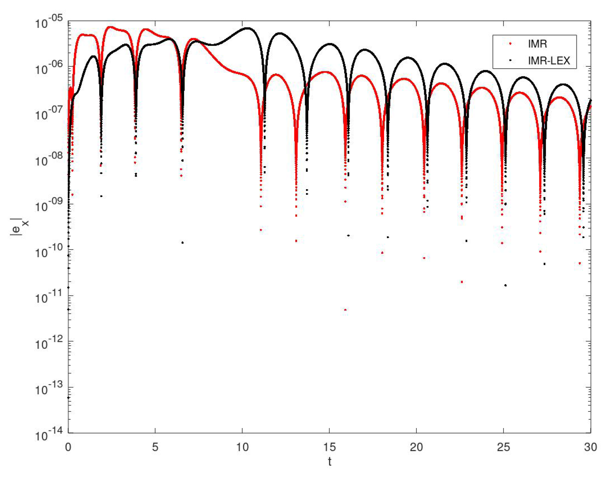
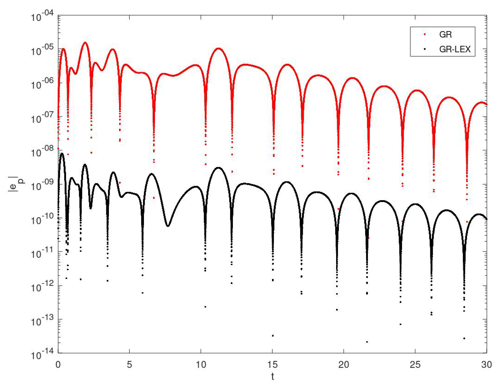
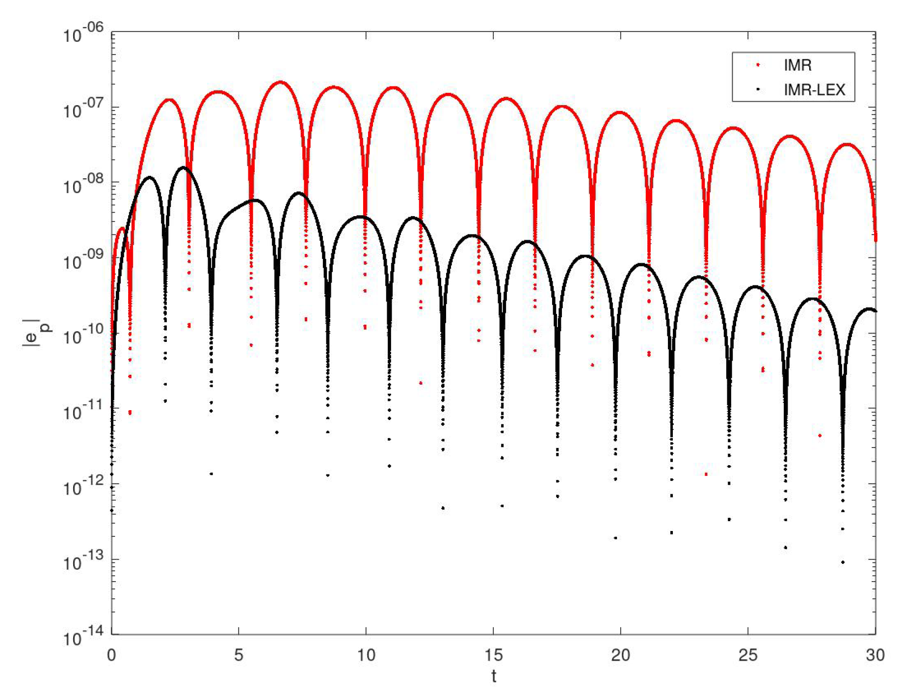
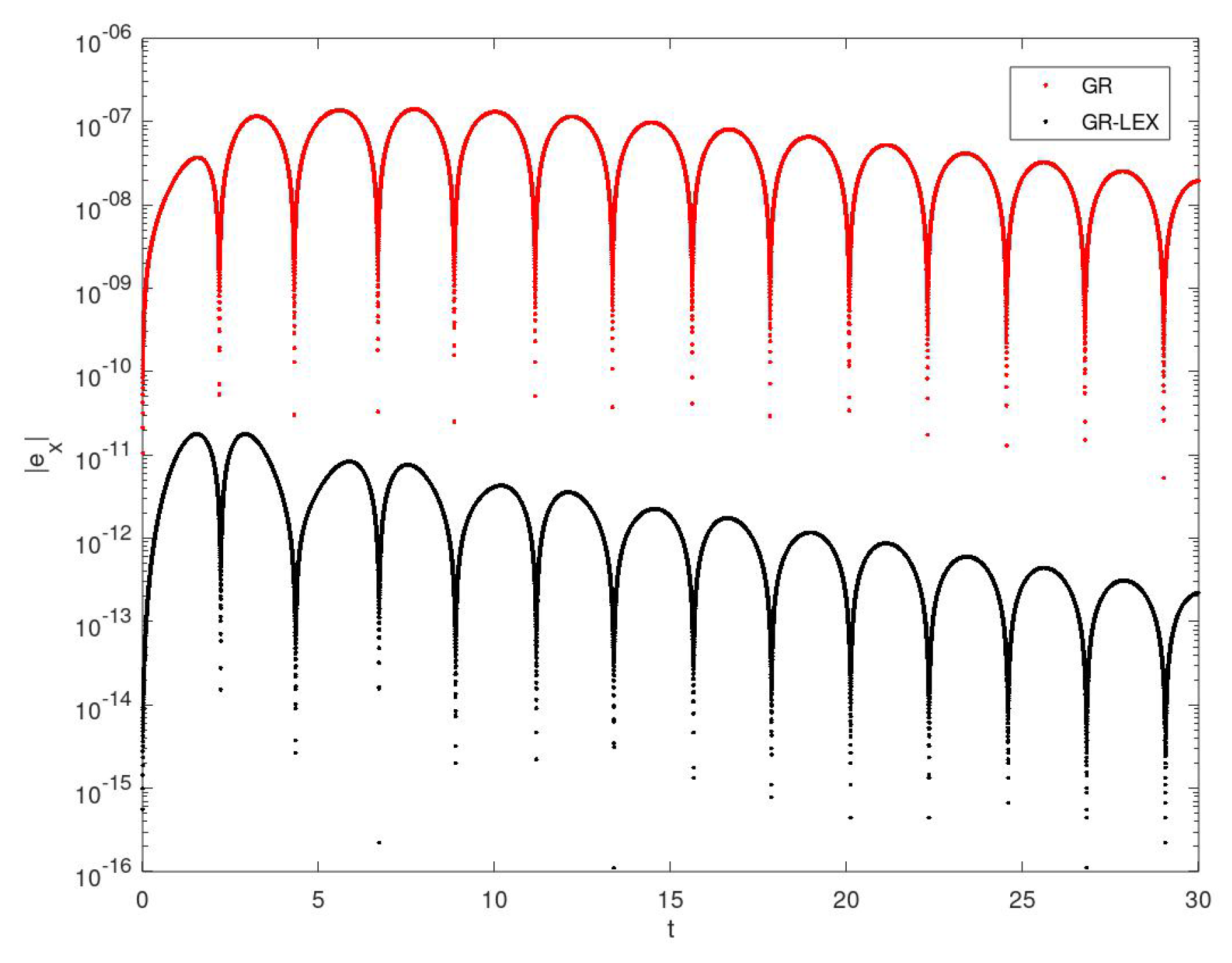
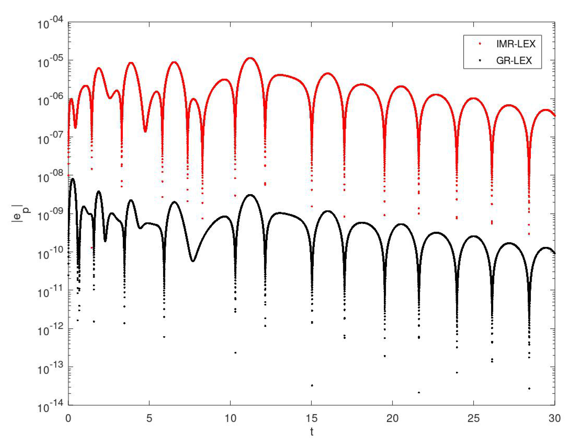
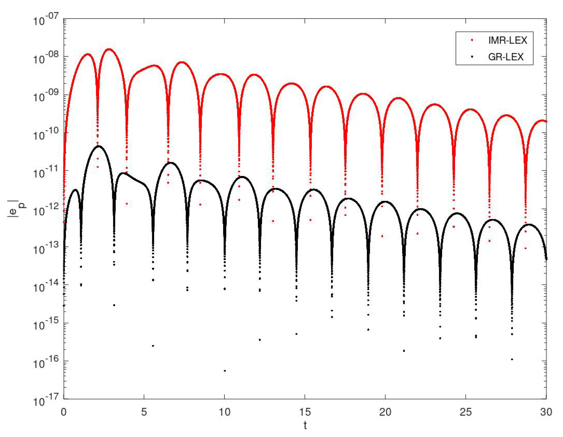
The locally exact modification is not very useful in the case of the implicit midoint rule for generic initial conditions. In fact it even worsens the performance of the algorithm, see Figure 1. The accuracy of the discrete gradient scheme for the same initial conditions is improved by about 3 orders of magnitude, see Figure 2. The situation changes for trajectories in the vicinity of the stable equilibrium. Here locally exact modifications improve both algorithms, although the improvement is much greater in the case of the discrete gradient scheme, compare Figure 3 with Figure 4. The advantage of the GR-LEX method in comparison to IMR-LEX is clearly shown at Figure 5 and Figure 6.

7. Concluding Remarks

We studied two locally exact integrators for the Duffing equation: locally exact discrete gradient scheme (GR-LEX) and locally exact implicit midpoint rule (IMR-LEX). The first one has two important advantages. It is of the third order (hence more accurate than GR and IMR schemes) and it preserves the geometric properties of the Duffing equation (the discretized Lapunov function is strictly monotonic, exactly as in the continuous case).

Numerical experiments confirm the enhanced accuracy of the GR-LEX scheme for all studied initial conditions. On the other hand, IMR-LEX is, in general, of similar accuracy as unmodified IMR (in the same time being more expensive). However, for initial conditions in a neighbourhood of the stable equilibrium, this method becomes much more accurate that IMR (we claim that this is a feature of any locally exact scheme).

References

- Cieśliński, J.L. Locally exact modifications of discrete gradient schemes. Phys. Lett. A 2013, 377, 592–597. [Google Scholar] [CrossRef]
- Cieśliński, J.L. Locally exact modifications of numerical schemes. Comput. Math. Appl. 2013, 65, 1920–1938. [Google Scholar] [CrossRef]
- Potts, R.B. Differential and difference equations. Am. Math. Mon. 1982, 89, 402–407. [Google Scholar] [CrossRef]
- Agarwal, R.P. Difference Equations and Inequalities; Marcel Dekker: New York, NY, USA, 2000; Chapter 3. [Google Scholar]
- Mickens, R.E. Nonstandard Finite Difference Models of Differential Equations; World Scientific: Singapore, 1994. [Google Scholar]
- Hairer, E.; Lubich, C.; Wanner, G. Geometric Numerical Integration: Structure-preserving Algorithms for Ordinary Differential Equations, 2nd ed.; Springer: Berlin, Germany, 2006. [Google Scholar]
- Hochbruck, M.; Lubich, C. A Gautschi-type method for oscillatory second-order differential equations. Numer. Math. 1999, 83, 403–426. [Google Scholar] [CrossRef] [Green Version]
- Celledoni, E.; Cohen, D.; Owren, B. Symmetric exponential integrators with an application to the cubic Schrödinger equation. Found. Comput. Math. 2008, 8, 303–317. [Google Scholar] [CrossRef]
- Hochbruck, M.; Ostermann, A. lExponential integrators. Acta Numer. 2010, 19, 209–286. [Google Scholar] [CrossRef] [Green Version]
- Cieśliński, J.L. Improving the accuracy of the AVF method. J. Comput. Appl. Math. 2014, 259 Pt A, 233–243. [Google Scholar] [CrossRef]
- McLachlan, R.I.; Quispel, G.R.W.; Tse, P.S.P. Linearization-preserving self-adjoint and symplectic integrators. BIT Numer. Math. 2009, 49, 177–197. [Google Scholar] [CrossRef]
- Cieśliński, J.L.; Ratkiewicz, B. Long-time behaviour of discretizations of the simple pendulum equation. J. Phys. A Math. Theor. 2009, 42, 105204. [Google Scholar] [CrossRef]
- Greenspan, D. An algebraic, energy conserving formulation of classical molecular and Newtonian n-body interaction. Bull. Am. Math. Soc. 1973, 79, 423–427. [Google Scholar] [CrossRef] [Green Version]
- McLachlan, R.I.; Quispel, G.R.W.; Robidoux, N. Geometric integration using discrete gradients. Philos. Trans. R. Soc. Lond. A 1999, 357, 1021–1045. [Google Scholar] [CrossRef]
- Iserles, A. A First Course in the Numerical Analysis of Differential Equations; Cambridge Univ. Press: Cambridge, UK, 2009. [Google Scholar]
- Cieśliński, J.L.; Ratkiewicz, B. On simulations of the classical harmonic oscillator equation by difference equations. Adv. Difference Eqs. 2006, 2006, 40171. [Google Scholar] [CrossRef] [Green Version]
- Cieśliński, J.L.; Ratkiewicz, B. Energy-preserving numerical schemes of high accuracy for one-dimensional Hamiltonian systems. J. Phys. A Math. Theor. 2011, 44, 155206. [Google Scholar] [CrossRef]
- Niesen, J.; Wright, W.M. Algorithm 919: A Krylov subspace algorithm for evaluating the φ-functions appearing in exponential integrators. ACM Trans. Math. Softw. 2012, 38, 22. [Google Scholar] [CrossRef] [Green Version]
- Cieśliński, J.L. Comment on ‘Conservative discretizations of the Kepler motion’. J. Phys. A Math. Theor. 2010, 43, 228001. [Google Scholar] [CrossRef]
- Cieśliński, J.L. On the exact discretization of the classical harmonic oscillator equation. J. Difference Equ. Appl. 2011, 17, 1673–1694. [Google Scholar] [CrossRef]
- Bader, P.; Blanes, S. Fourier methods for the perturbed harmonic oscillator in linear and nonlinear Schrödinger equations. Phys. Rev. 2011, E83, 046711. [Google Scholar] [CrossRef] [Green Version]
- Cieśliński, J.L.; Ratkiewicz, B. Improving the accuracy of the discrete gradient method in the one-dimensional case. Phys. Rev. E 2010, 81, 016704. [Google Scholar] [CrossRef] [Green Version]
- Cieśliński, J.L.; Ratkiewicz, B. Discrete gradient algorithms of high-order for one-dimensional systems. Comput. Phys. Commun. 2012, 183, 617–627. [Google Scholar] [CrossRef] [Green Version]
- Pope, D.A. An exponential method of numerical integration of ordinary differential equations. Commun. ACM 1963, 6, 491–493. [Google Scholar] [CrossRef]
- Zhang, J.J. Locally exact discretization method for nonlinear oscillation systems. J. Low Freq. Noise Vibrat. Active Control 2019, 38, 1567–1575. [Google Scholar] [CrossRef] [Green Version]
- Diele, F.; Marangi, C. Geometric Numerical Integration in Ecological Modelling. Mathematics 2020, 8, 25. [Google Scholar] [CrossRef] [Green Version]
- Gonzales, O. Time integration and discrete Hamiltonian systems. J. Nonl. Sci. 1996, 6, 449–467. [Google Scholar] [CrossRef]
- Kobus, A. Computational enhancement of discrete gradient method. arXiv 2019, arXiv:1912.07253. [Google Scholar]
- Kovacic, I.; Brennan, M.J. (Eds.) The Duffing Equation. Nonlinear Oscillators and Their Behaviour; Wiley & Sons: Hoboken, NJ, USA, 2011. [Google Scholar]
Figure 1.
Errors of IMR-LEX (black) compared to errors of IMR (red) for generic initial conditions .
Figure 2.
Errors of GR-LEX (black) compared to errors of GR (red) for generic initial conditions .
Figure 3.
Errors of IMR-LEX (black) compared to errors of IMR (red) near equilibrium: , .
Figure 4.
Errors of GR-LEX (black) compared to errors of GR (red) near equilibrium: , .
Figure 5.
Errors of GR-LEX (black) and errors of IMR-LEX (red) for generic initial conditions , .
Figure 6.
Errors of GR-LEX (black) compared to errors of IMR-LEX (red) near equilibrium: , .
© 2020 by the authors. Licensee MDPI, Basel, Switzerland. This article is an open access article distributed under the terms and conditions of the Creative Commons Attribution (CC BY) license (http://creativecommons.org/licenses/by/4.0/).
Share and Cite
MDPI and ACS Style
Cieśliński, J.L.; Kobus, A. Locally Exact Integrators for the Duffing Equation. Mathematics 2020, 8, 231. https://doi.org/10.3390/math8020231
AMA Style
Cieśliński JL, Kobus A. Locally Exact Integrators for the Duffing Equation. Mathematics. 2020; 8(2):231. https://doi.org/10.3390/math8020231
Chicago/Turabian StyleCieśliński, Jan L., and Artur Kobus. 2020. "Locally Exact Integrators for the Duffing Equation" Mathematics 8, no. 2: 231. https://doi.org/10.3390/math8020231
Note that from the first issue of 2016, this journal uses article numbers instead of page numbers. See further details here.