Impact of Heat Generation on Magneto-Nanofluid Free Convection Flow about Sphere in the Plume Region


1
Department of Mathematics, Faculty of Science, University of Sargodha, Sargodha 40100, Pakistan
2
Department of Mathematics, Faculty of Science, Aswan University, Aswan 81528, Egypt
3
Department of Mathematics, College of Science and Humanities in Al-Kharj, Prince Sattam Bin Abdulaziz University, Al-Kharj 11942, Saudi Arabia
4
Department of Basic Engineering Science, Faculty of Engineering, Menoufia University, Shebin El Kom 32511, Egypt
*
Author to whom correspondence should be addressed.
Mathematics 2020, 8(11), 2010; https://doi.org/10.3390/math8112010
Submission received: 12 October 2020
/
Revised: 7 November 2020
/
Accepted: 9 November 2020
/
Published: 11 November 2020
(This article belongs to the Special Issue Computational Fluid Dynamics 2020)
Abstract
:The main aim of the current study is to analyze the physical phenomenon of free convection nanofluids heat transfer along a sphere and fluid eruption through boundary layer into a plume region above the surface of the sphere. In the current study, the effect of heat generation with the inclusion of an applied magnetic field by considering nanofluids is incorporated. The dimensioned form of formulated equations of the said phenomenon is transformed into the non-dimensional form, and then solved numerically. The developed finite difference method along with the Thomas algorithm has been utilized to approximate the given equations. The numerical simulation is carried out for the different physical parameters involved, such as magnetic field parameter, Prandtl number, thermophoresis parameter, heat generation parameter, Schmidt number, and Brownian motion parameter. Later, the quantities, such as velocity, temperature, and mass distribution, are plotted under the impacts of different values of different controlling parameters to ascertain how these quantities are affected by these pertinent parameters. Moreover, the obtained results are displayed graphically as well in tabular form. The novelty of present work is that we first secure results around different points of a sphere and then the effects of all parameters are captured above the sphere in the plume.
1. Introduction
The conventional fluids, such as mixtures of ethylene glycol, oil, and water, have been used for the purpose of heat transportation by the research community. The heat transfer process was made very slow by the use of these fluids due to their poor thermal conductivity. The utilization of nanofluids as a cooling source increases operating and manufacturing costs. So, nanofluids are being used to speed up the heat transfer performances because of their excellent thermal conductivity. Nanofluids result from the suspension of submicron solid particles (nanoparticles) in the base fluids, such as water or any organic solvent. Nanoparticles are of growing interest as they play an effective role to strengthen the thermal conductivity of the base fluid. The inclusion of a magnetic field in the analysis of nanofluids has attracted much attention of researchers because of its growing applications in the fields of engineering, physics, and chemistry. The nanofluids which contain magnetic particles act as super-paramagnetic fluids which absorb the energy control of the flow and act as an alternating electromagnetic field. Nanofluids are employed as coolants in computer microchips and many other electronic devices which utilize micro-fluidic applications. With motivation from the above applications of magnetohydrodynamic flow, Sparrow and Cess [1] comprehensively analyzed the study of magnetohydrodynamic natural convection flow through the vertical plate by encountering both upward and downward flows with the effect of buoyancy forces. Potter and Riley [2] focused their attention on natural convection flow due to a heated sphere placed in static fluid by considering large values of the Grashof number. They discussed the characteristics of boundary layer flow into the plume numerically. Riley [3] considered the phenomenon of free convection flow along the surface of a sphere by maintaining higher temperature than the surroundings. He evaluated the model numerically for finite values of Grashof and Parndtl numbers. Andersson [4] studied the model of visco-elastic fluid over the stretching surface considering the effect of a transverse magnetic field analytically. Stephen and Eastman [5] proposed a novel type of fluid whose thermal conductivity is higher than conventional fluids and termed them as nanofluids. They concluded that such types of fluid enhance the thermal performances during the process of heat transfer. Samuel and Falade [6] investigated the stability of hydromagnetic fluid in porous media by incorporating the outcomes of variable viscosity. Their prediction for theoretical analysis was that an increase in the viscosity variation parameter creates a stability of the fluid flow. The transient form of the convective flow along the surface of a moving plate in a porous medium with uniform heat flux with the inclusion of a magnetic field has been studied by Al-Kabeir et al. [7]. Chamkha and Aly [8] presented nanofluids flow by means of free convection heat transfer over the permeable plate observing a magnetic field, transpiration parameter, heat absorption, and generation influences for main physical properties. The phenomenon of double diffusive free convection nanofluids flow over the vertical plate was examined in [9]. Rosmilaet al. [10] studied the problem of free convection magnetohydrodynamic flow of nanofluids over a linearly stretching surface by the opting shooting technique along with the Runge–Kutta method of the fourth order. Mohammad et al. [11] analyzed the flow problem of a magnetohydrodynamic boundary layer over a vertical surface for nanofluids taking into account Newtonian heating effects. Gandhar and Reddy [12] predicted heat and mass transfer mechanism for moving plate held vertically embedded in porous media due to the insertion of magnetic field. The analysis on the influences of buoyancy force, magnetic field, and a stretching and shrinking sheet on the stagnation point flow of nanofluids was performed by Makinde et al. [13]. Olanrewaju and Makinde [14] discussed the problem of natural convection flow of nanofluids over a porous surface with a stagnation point in the presence of Newtonian heating effects. Chamkha et al. [15] reviewed the available material properties of nanofluids and focused on several geometries and applications. Stagnation point flow on a vertical stretching surface by imposing the slip condition was discussed by Khairy and Ishak [16]. The analysis of the nanofluids in the presence of a chemical reaction and magnetic field has been carried by Ltu and Ochsnor [17]. Another study was conducted to assess the free convection flow of nanofluids about different circumferential points of a sphere and the fluid erupting from the boundary layer flow into the plume made above the sphere [18]. The characteristics of heat and fluid flow in the presence of nanofluids have been investigated by [19,20,21,22,23,24,25] along different simple and complex geometries.
With inspiration from aforesaid research attempts, we intended to elaborate the problem of natural convective flow of magnetohydrodynamic nanofluids flow at the different circumferential positions along the surface of a sphere and into the plume made above the sphere by encountering the effects of heat generation and absorption. It is necessary to highlight that no one has paid any attention towards such a problem before this attempt. In the subsequent sections, the mathematical formulation is performed and after suitable transformation of the modeled equations, a very accurate approximating technique known as the finite difference method is directly employed to get the approximate solutions of the partial differential equations. By using FORTRAN as a computing tool, asymptotic and valid solutions of the governing model satisfying the given boundary conditions are calculated. Further, in this study, the different trends/behaviors depending on various combinations of many influential parameters have been displayed graphically as well as in tabular form.
2. Statement of the Problem and Mathematical Formulation
Consider a steady, two-dimensional, viscous, incompressible, and electrically conducting boundary layer flow of nanofluid. In this analysis, water is taken as the base fluid and heat generation effects are encountered. The physical sketch and geometry of the problem are shown in Figure 1. The sphere surface is kept at constant temperature and the nanoparticles volume fraction at the surface is . The coordinate along the surface of a sphere is and is taken as normal to the surface. The corresponding velocity components and is considered along and normal to the surface of the sphere respectively. There are three regions, namely sphere, fluid erupting from the boundary layer, and plume made above the sphere. The universal conservation equations for the current mechanism following Potter and Riley [2] take the forms given as below:
Subjected to the corresponding boundary conditions:
The symbols appeared in the above governing equations such as , and are termed as gravitational acceleration, thermal expansion of temperature, thermal diffusivity, nanoparticles heat capacity to base fluid ratio and solutal thermal expansion. The Brownian diffusion coefficient, heat generation coefficient, thermophoretic diffusion coefficient, and magnetic field strength are denoted by , and , respectively. To make the above proposed model dimensionless, here, non-dimensionless variables are defined as below:
where is the sphere radius. By inserting Equation (6) into Equations (1)–(5), we obtain the following non-dimensional forms of the governing equations as given below:
With boundary conditions:
where
The parameters appearing above are the thermophoresis parameter, Schmidt number, Prandtl number, and Brownian motion parameter, which are designated , and . Here, , and represent the magnetic field parameter and heat generation parameter, respectively.
3. Method of Solution
To adopt an ease in making the algorithm, the following primitive variables are used to make the primitive form of the above Equations (7)–(10) along with boundary conditions:
After substitution of the variables defined in Equation (12) into Equations (7)–(11), we get the following primitive system of partial differential equations:
The corresponding boundary conditions are:
4. Computational Scheme
The formulated model is complex and its analytical solution cannot be found. So, we move towards the approximate solutions of the present problem with the use of very accurate approximating technique known as finite difference method. This method is directly applied to partial differential Equations (13)–(17) to convert into algebraic system of equations which is solved by coding on computing tool FORTRAN package. The backward difference is used along -axis and central difference along -axis. The discretization procedure is given below:
The insertion of Equations (18)–(20) into Equations (13)–(17) implies:
With boundary conditions:
5. Governing Equations for Plume Region
Considering the diagram of the geometry, we can see that nanofluid enters from the region-II to region-III. For this region, the aforesaid model is altered and a new model for the plume region is formulated by following [2]:
With boundary conditions:
Dimensionless variables:
Dimensionless form of system of equations:
With boundary conditions:
For the convenient form of the integration, we use the following variables for the required form:
Using the above primitive variable formulation, we have the following system of equations:
With boundary conditions:
Solution Methodology
For the numerical evaluation of the flow equations in the plume region, the finite difference scheme is implemented. The constitutive equations in discretized forms are given as below:
With boundary conditions:
6. Analysis of the Results
This section covers the discussion and conclusion on the behaviors of velocity field , temperature field , and mass field , along with heat transfer rate , mass transfer rate , and skin friction with the variations of different flow parameters. The effects of parameters which are taken into observation are named as magnetic field parameter, , heat generation parameter, Schmidt number, Sc, Prandtl numbers, Pr, thermophoresis parameter, , and Brownian motion parameter, . The obtained numerical solutions for considered governing properties are displayed in graphical form and tabulated as well. The solution detail has been split into two parts, i.e., the several locations around a sphere and in the plume region above the sphere.
6.1. Fluxes and Boundary Layers on the Sphere
In this subsection, we are going to present and discuss the obtained solutions at different circumferential stations around the surface of a sphere. The result demonstrated in Figure 2a–c are for velocity, temperature, and mass profiles with the variations of Schmidt number keeping the remaining parameters constant at different circumferential positions of a sphere. It can be viewed that, as the Schmidt number is increased at the considered positions of a sphere, that is X = 0.1, 1.0, 2.0, and 3.0, velocity and mass profiles go down, but the opposite behavior is observed in the temperature field. In addition, it is necessary to mention that maximum magnitude for velocity distribution is achieved at position X = 1.0, but for temperature and mass concentration, it is obtained at X = 3.0. In these graphs, the simultaneous momentum and mass diffusion convection processes have been highlighted very clearly. Figure 3a,b depicts the results for velocity, temperature field, and mass concentration corresponding to increasing values of heat generation parameter Q and the remaining parameters treated as fixed at several stations of a sphere. We can see that the temperature and mass distributions have decreasing behavior, but the opposite phenomenon is observed in the velocity distribution. One aspect which is necessary to highlight is that very minor variations are observed for temperature and velocity fields, but a reasonable change is found in mass distribution at the taken circumferential positions of a sphere. From these graphs, it is evident that the heat generation parameter balances the heat transfer mechanism in the fluid flow domain. Figure 4a–c represents the behavior of the aforesaid physical properties for different values of the Prandtl number Pr. The outcomes shown in Figure 4a–c imply that, owing to the enhancement of Prandtl number at different circumferential locations of a sphere, a decrease in mass and velocity distributions, but an increase in temperature distribution, are noted. It is necessary to mention that the highest magnitude for velocity is gained at circumferential points X = 1.0, while on the other hand, mass and temperature distribution secure the peak value at position X = 3.1. As the Prandtl number controls the relative thickness of the momentum and thermal boundary layer, when Pr is small, the heat diffuses quickly as compared to the velocity. The effects of Brownian motion parameters on the physical properties mentioned earlier are presented in Figure 5a–c. It is noteworthy to point out that the augmentation in the Brownian motion parameter gives birth to a rise in mass distribution, but no remarkable variations are noted in the temperature and velocity fields. Figure 6a–c highlight the outcomes of profiles of velocity, temperature, and mass concentration under the action of diverse values of magnetic field parameter. It can be noticed that fluid velocity slows down as magnetic field parameter M is increased from 0.2 to 0.8 at each contemplated point around our proposed geometry and the temperature profile and mass concentration get smaller magnitudes for the same values of the parameters and positions. It is a point of interest that top values for flow velocity are maintained at X = 1.0 and for temperature and mass distribution, the highest values are gained at position X = 3.0. Variations in fluid velocity, temperature field, and mass concentration for increasing values of the thermophoresis parameter are demonstrated in Figure 7a–c. Very profound results are determined for all proposed properties. It is worthy to mention that the velocity of the fluid and temperature are reduced for increasing values of thermophoresis parameter Nt at the proposed positions about the surface of a sphere. On the other hand, for the same parametric conditions, mass concentration is enhanced. In Figure 8a–c, heat and mass transfer rates with skin friction are plotted. Interestingly, it can be seen that the heat transfer rate grows well, but mass transfer and skin friction become weaker at every contemplated circumferential point of a sphere. Similar properties as discussed earlier are taken under discussion and displayed in Figure 9a–c. Benchmark results for velocity, temperature, and solutal gradients for different values of Prandtl number have been studied at various stations of a sphere. There is a reduction in skin friction and mass transfer, but an increment in heat transfer rate is noted. The results tabulated in Table 1 represents skin friction, heat transfer rate and mass transfer for varying values of Brownian motion parameter. The outcomes in Table 1 imply that skin friction get reduced whereas heat and mass transfer rates go up as is augmented at the proposed stations of a sphere. Table 2 is reflecting the influences of magnetic field parameter on aforementioned material properties. By making larger the values of magnetic field parameter all contemplated material properties get declined. Further, it is concluded that greatest magnitudes for skin friction, rate of heat transfer and mass transfer rate are assured at positions X = 2.0, X = 1.0, and X = 1.0, respectively. Heat generation effects on velocity gradient, heat transfer rate and mass transfer rate are illustrated in Table 3. We can claim from the displayed results that skin friction and mass transfer enhance, but the converse phenomenon occurred for the case of heat transfer. In Table 4, the impact of Schmidt number is shown. Tabulated results show that skin friction falls down, but the mass transfer rate and heat transfer rate are augmented.
6.2. Fluxes and Boundary Layers in the Plume Region
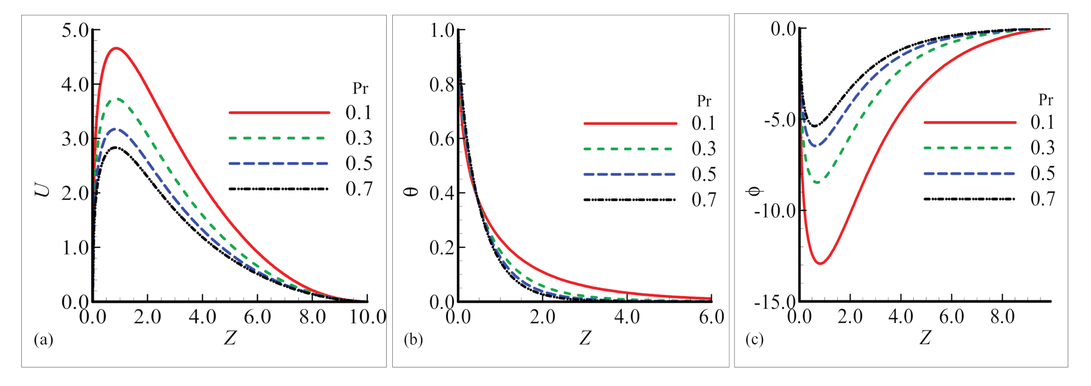
The present subsection deals with the analysis and demonstration of the numerical solutions of the flow model developed for the case of the plume region which occurs above the sphere. Figure 10a–c illustrate the temperature profile and nanoparticles volume fraction profile for various values of Schmidt number in the plume region. All the other parametric values are fixed. We can deduce from the figures that, as Sc is augmented from 0.3 to 0.9, velocity is lowered whereas temperature and nanoparticles volume fraction profiles curves go up. It was expected that the nanoparticles volume fraction will rise corresponding to an increase in Schmidt number Sc. The influences of thermophoresis parameter Nt, on the material properties are highlighted in Figure 11a–c. Computed results are reflecting that velocity of the flow field gets enhanced but temperature and nanoparticles volume fraction decline as Nt is increased. Graphical representations in Figure 12a–c are for the same substantial properties under the influence of several values of Brownian motion parameter Nb. It can be inferred from the displayed results that the velocity of the flow field goes down, nanoparticles volume fraction distribution goes up, but no variations are seen in the temperature field. Heat generation impacts by taking its several values on the conduct of matter properties, such as velocity, temperature, and nanoparticles volume fraction profiles, are examined in Figure 13a,b. From the sketched graphs, it is inferred that velocity and temperature field get larger magnitudes with the reduction in nanoparticles volume fraction by the augmentation of heat generation parameter Q. The results according to expectation satisfy the given boundary conditions and approach to the targets asymptotically. The graphs in Figure 14a–c are sketched for many values of magnetic field parameter M. It can be deduced from these plots that flow velocity and nanoparticles volume fraction rise, but no difference is found in the temperature field. The effects of various values of Prandtl number Pr on the already mentioned material properties are elaborated graphically in Figure 15a–c. We can see that velocity and temperature distributions decrease but nanoparticles volume fraction increases owing to increasing values of Pr. It was obvious that there is a reduction in field velocity and temperature profile.
7. Conclusions
The phenomena of steady laminar natural convection nanofluid flow around the surface of a sphere and in the plume region are numerically examined under the impact of heat generation and an applied magnetic field. We summarize the obtained results in the following lines.
- The Schmidt number exerted a noticeable influence on the heat and fluid flow mechanism around the surface of the sphere and in the plume region in terms of velocity profile, temperature profile, and mass concentration.
- It was found that, under the action of diverse values of magnetic field parameter, the velocity of fluid slows down as the magnetic field parameter increased from 0.2 to 0.8, while on the other hand, the temperature profile and mass concentration became smaller in magnitude for the same values of the parameters and positions.
- The effect of thermophoresis parameter Nt cannot be neglected, as due to an increase in the magnitude of this parameter, the velocity profile is maximum at position X = 1.0, while the heat and mass transfer are reduced at the same position.
- The variation in the Brownian motion parameter Nb results in distinct changes in the thermal and flow field, depending on different positions around the surface of the sphere and in the plume region. The Brownian motion demonstrated its increasing effect for velocity at position X = 1.0, and dominated at the same position for temperature distribution and mass concentration.
- The graphs sketched in the plume region for many values of magnetic field parameter M show that the flow velocity and nanoparticles volume fraction rise, but no difference is found in the temperature field. The numerical solution obtained around the sphere reflects the influence of the magnetic field parameter on the aforementioned material properties, i.e., increasing the values of the magnetic field parameter.
- The Prandtl number Pr largely effects the fluid and thermal characteristics in the prescribed domain of study.
- From the obtained results of velocity profile, temperature distribution, and mass concentration around the sphere and within the plume region, it is observed that all the results are satisfied by the subjected boundary conditions.
Author Contributions
Conceptualization, A.K. and M.A.; Supervision, M.A. and H.A.N.; Investigation, A.N. and A.M.R.; Methodology, A.K., M.A. and H.A.N.; Writing—original draft, A.K., M.A. and H.A.N.; Writing—review & editing, M.A., A.M.R. and H.A.N.; Software, A.K., M.A. and A.M.R.; Formal Analysis, A.K., M.A., A.M.R. and H.A.N. All authors have read and agreed to the published version of the manuscript.
Funding
This research received no external funding.
Conflicts of Interest
The authors declare no conflict of interest.
Abbreviations
| Dimensioned velocity component in direction | |
| Dimensioned velocity component in direction | |
| Dimensioned velocity component in direction | |
| Dimensioned axes along and normal to the surface of a sphere | |
| Measured radially from the plume axis | |
| Primitive variable for velocity component in direction | |
| Primitive variable for velocity component in direction | |
| Gravitational acceleration | |
| Fluid temperature in boundary layer | |
| Mass concentration in boundary layer | |
| Specific heat at constant pressure | |
| The radius of a sphere | |
| Dimensioned radial distance from the symmetric axis to the surface of a sphere | |
| Mass diffusion cefficient | |
| Greek Symbols | |
| Volumetric coefficient thermal expansion | |
| Thermophoretic diffusion coefficient | |
| Volumetric coefficient concentration expansion | |
| Thermal diffusivity | |
| Dimensionless temperature | |
| Dimensionless mass concentration | |
| Dynamic viscosity | |
| Density of the particle | |
| Kinematic viscosity | |
| Fluid density | |
| Thermal conductivity | |
| Subscripts | |
| Ambient conditions | |
| Wall conditions | |
References
- Sparrow, E.M.; Cess, R.D. The effect of the magnetic field on free convection heat transfer. Int. J. Heat Mass Transfer. 1961, 3, 267–274. [Google Scholar]
- Potter, J.M.; Riley, N. Free convection from a heated sphere at large Grashof number. J. Fluid Mech. 1980, 100, 769–783. [Google Scholar] [CrossRef]
- Riley, N. The heat transfer from a sphere in free convective flow. Comput. Fluids. 1986, 14, 225–237. [Google Scholar]
- Andersson, H.I. MHD flow of a viscoelastic fluid past a stretching surface. ActaMechanica 1992, 95, 227–230. [Google Scholar]
- Choi, S.U.S.; Eastman, J.A. Enhancing Thermal Conductivity of Fluids with Nanoparticles; Argonne National Lab.: DuPage County, IL, USA, 1995. Available online: https://www.osti.gov/servlets/purl/196525 (accessed on 20 October 2020).
- Adesanya, S.O.; Falade, J.A. Hydrodynamic stability analysis for variable viscous fluid flow through a porous medium. Int. J. Differ. Equ. 2014, 13, 219–230. [Google Scholar]
- El-Kabeir, S.M.M.; Rashad, A.M.; Gorla, R.S.R. Unsteady MHD combined convection over a moving vertical sheet in a fluid saturated porous medium with uniform surface heat flux. Math. Comp. Model 2007, 46, 384–397. [Google Scholar] [CrossRef]
- Chamkha, A.J.; Aly, A.M. MHD free convection flow of a nanofluid past a vertical plate in the presence of heat generation or absorption effects. Chem. Eng. Commun. 2010, 198, 425–441. [Google Scholar]
- Kuznetsov, A.V.; Nield, D.A. Double-diffusive natural convective boundary-layer flow of nanofluids past a vertical plate. Int. J. Therm. Sci. 2011, 50, 712–717. [Google Scholar]
- Rosmila, A.B.; Kandasamy, R.; Muhaimin, I. Lie symmetry group transformation for MHD natural convection flow of nanofluid over linearly porous stretching sheet in presence of thermal stratification. Appl. Math. Mech. 2012, 33, 593–604. [Google Scholar] [CrossRef] [Green Version]
- Uddin, M.J.; Khan, W.A.; Ismail, A.I. MHD free convective boundary layer flow of a nanofluid past a flat vertical plate with Newtonian heating boundary condition. PLoS ONE 2012, 7, e49499. [Google Scholar]
- Gangadhar, K.; Reddy, B. Chemically reacting MHD boundary layer flow of heat and mass transfer over a moving vertical plate in a porous medium with suction. J. Appl. Fluid Mech. 2013, 6, 107–114. [Google Scholar]
- Makinde, O.D.; Khan, W.A.; Khan, Z.H. Buoyancy effects on MHD stagnation point flow and heat transfer of a nanofluid past a convectively heated stretching/shrinking sheet. Int. J. Heat Mass Transfer. 2013, 62, 526–533. [Google Scholar] [CrossRef]
- Olanrewaju, A.M.; Makinde, O.D. On boundary layer stagnation point flow of a nanofluid over a permeable flat surface with Newtonian heating. Chem. Eng. Commun. 2013, 200, 836–852. [Google Scholar] [CrossRef]
- Chamkha, A.J.; Jena, S.K.; Mahapatra, S.K. MHD convection of nanofluids: A review. J. Nanofluids 2015, 4, 271–292. [Google Scholar] [CrossRef]
- Zaimi, K.; Ishak, A. Stagnation-point flow towards a stretching vertical sheet with slip effects. Mathematics 2016, 4, 27. [Google Scholar] [CrossRef]
- Itu, C.; Öchsner, A.; Vlase, S.; Marin, M.I. Improved rigidity of composite circular plates through radial ribs. Proc. Inst. Mech. Eng., Part L J. Mater. Des. Appl. 2019, 233, 1585–1593. [Google Scholar] [CrossRef]
- Ashraf, M.; Khan, A.; Gorla, R.S.R. Natural convection boundary layer flow of nanofluids around different stations of the sphere and into the plume above the sphere. Heat Transf. Asian Res. 2019, 48, 1127–1148. [Google Scholar] [CrossRef]
- Sheikholeslami, M.; Abelman, S.; Ganji, D.D. Numerical simulation of MHD nanofluid flow and heat transfer considering viscous dissipation. Int. J. Heat Mass Transf. 2014, 79, 212–222. [Google Scholar] [CrossRef]
- Qureshi, M.Z.A.; Rubbab, Q.; Irshad, S.; Ahmad, S.; Aqeel, M. Heat and mass transfer analysis of mhd nanofluid flow with radiative heat effects in the presence of spherical au-metallic nanoparticles. Nanoscale Res. Lett. 2016, 11, 472. [Google Scholar] [CrossRef] [Green Version]
- Myers, T.G.; Ribera, H.; Cregan, V. Does mathematics contribute to the nanofluid debate? Int. J. Heat Mass Transf. 2017, 111, 279–288. [Google Scholar] [CrossRef] [Green Version]
- Tlili, I.; Khan, W.A.; Ramadan, K. MHD flow of nanofluid flow across horizontal circular cylinder: Steady forced convection. J. Nanofluids 2019, 8, 179–186. [Google Scholar] [CrossRef]
- Khan, W.A.; Rashad, A.M.; Abdou, M.M.M.; Tlili, I. Natural bioconvection flow of a nanofluid containing gyrotactic microorganisms about a truncated cone. Eur. J. Mech.-B/Fluids 2019, 75, 133–142. [Google Scholar] [CrossRef]
- Parida, S.K.; Mishra, S.R. Heat and mass transfer of MHD stretched nanofluids in the presence of chemical reaction. J. Nanofluids 2019, 8, 143–149. [Google Scholar] [CrossRef]
- Khan, I.; Alqahtani, A.M. MHD nanofluids in a permeable channel with porosity. Symmetry 2019, 11, 378. [Google Scholar] [CrossRef] [Green Version]
Figure 1.
Coordinate System and Flow Geometry.

Figure 2.
Physical effects on quantities (a)
and (c) versus Sc when = 0.02, = 0.2, Pr = 0.72, M = 0.2, Q = 1.0.
Figure 2.
Physical effects on quantities (a)
and (c) versus Sc when = 0.02, = 0.2, Pr = 0.72, M = 0.2, Q = 1.0.

Figure 3.
Physical effects on quantities
and versus , when = 0.02, = 0.4, Pr = 0.72, M = 0.2, Sc = 1.0.
Figure 3.
Physical effects on quantities
and versus , when = 0.02, = 0.4, Pr = 0.72, M = 0.2, Sc = 1.0.
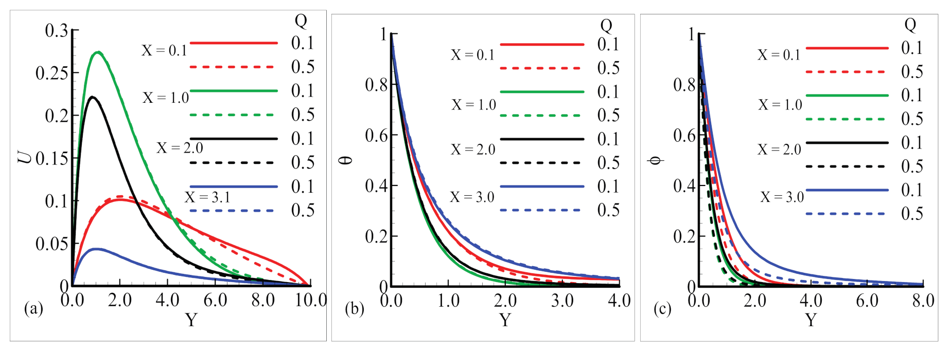
Figure 4.
Physical effects on quantities
and versus Pr, when = 0.02, = 0.4, = 1.0, M = 0.2,
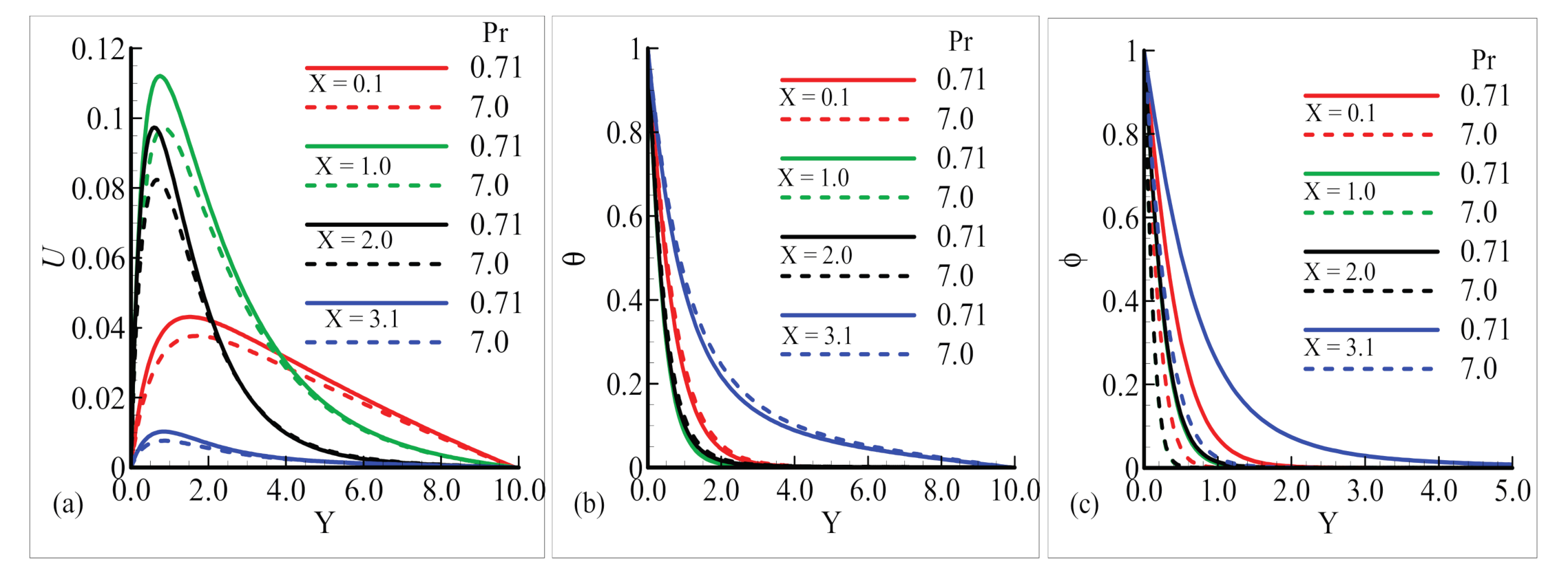
Figure 5.
Physical effects on quantities
and versus , when Nt = 0.02, = 1.0, = 7.0, M = 0.2, Q = 1.0.
Figure 5.
Physical effects on quantities
and versus , when Nt = 0.02, = 1.0, = 7.0, M = 0.2, Q = 1.0.
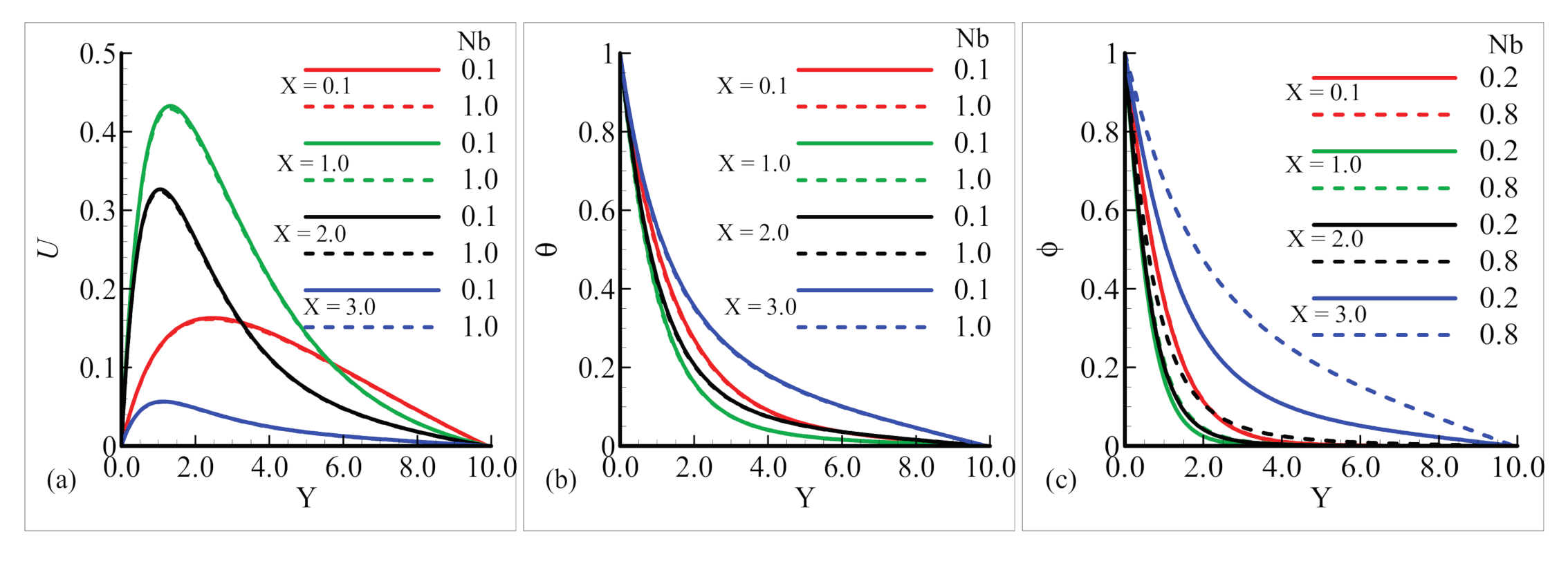
Figure 6.
Physical effects on quantities
and versus M, when = 0.02, = 0.4, Pr = 7.0, Sc = 10, Q = 1.0.
Figure 6.
Physical effects on quantities
and versus M, when = 0.02, = 0.4, Pr = 7.0, Sc = 10, Q = 1.0.
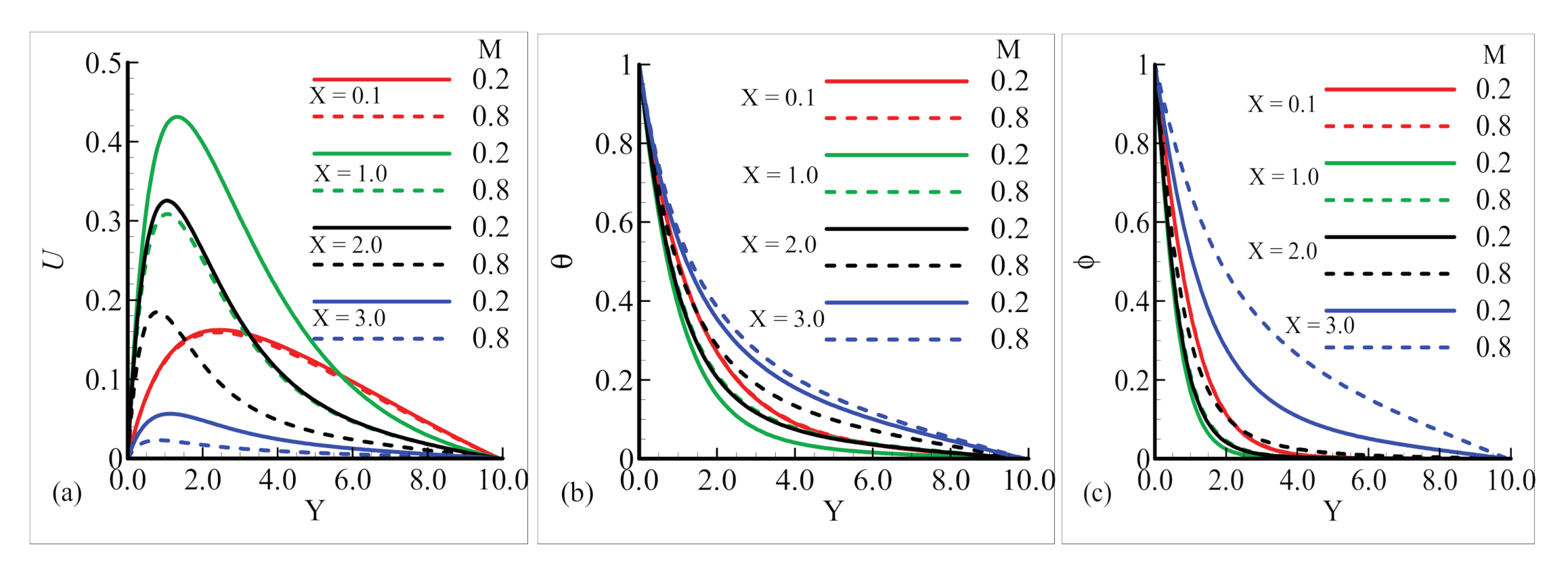
Figure 7.
Physical effects on quantities
and versus , when Sc = 1, = 0.4, = 7.0, M = 0.2, = 1.0.

Figure 8.
Physical effects on quantities
and versus, when Sc = 1.0, = 0.4, Pr = 7.0, M = 0.2, Q = 1.0.
Figure 8.
Physical effects on quantities
and versus, when Sc = 1.0, = 0.4, Pr = 7.0, M = 0.2, Q = 1.0.

Figure 9.
Physical effects on quantities
and versus, when Sc = 1.0, = 0.4, Pr = 0.2, M = 0.2, Q = 1.0.
Figure 9.
Physical effects on quantities
and versus, when Sc = 1.0, = 0.4, Pr = 0.2, M = 0.2, Q = 1.0.

Figure 10.
Physical effects on quantities and versus, when = 0.5, = 0.4, Pr = 0.71, M = 0.5, Q = 0.4.
Figure 10.
Physical effects on quantities and versus, when = 0.5, = 0.4, Pr = 0.71, M = 0.5, Q = 0.4.

Figure 11.
Physical effects on quantities
and versus , when = 0.8, = 0.4, Pr = 0.71, M = 0.4, Q = 0.2.
Figure 11.
Physical effects on quantities
and versus , when = 0.8, = 0.4, Pr = 0.71, M = 0.4, Q = 0.2.
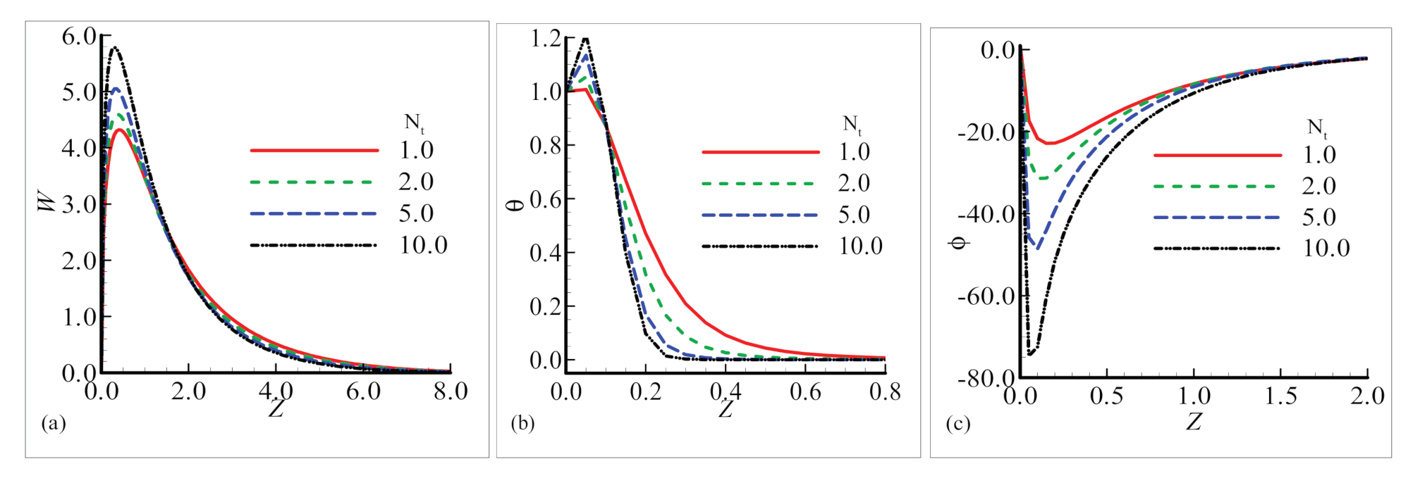
Figure 12.
Physical effects on quantities
and versus , when = 0.5, = 0.3, = 0.71, M = 0.4, Q = 0.4.
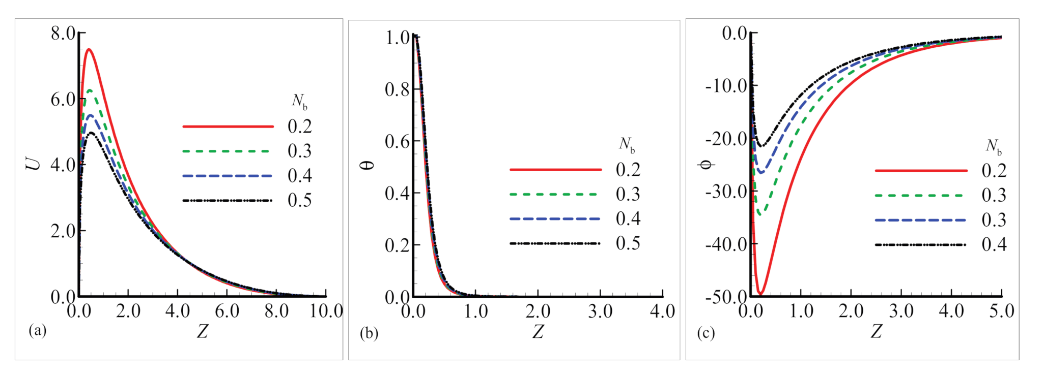
Figure 13.
Physical effects on quantities
and versus Q, when = 0.1, Nb = 0.4, Pr = 0.71, M = 0.2, = 0.2.
Figure 13.
Physical effects on quantities
and versus Q, when = 0.1, Nb = 0.4, Pr = 0.71, M = 0.2, = 0.2.

Figure 14.
Physical effects on quantities
and versus, when = 0.1, = 0.4, Pr = 0.71, Q = 0.2, Sc = 0.2.
Figure 14.
Physical effects on quantities
and versus, when = 0.1, = 0.4, Pr = 0.71, Q = 0.2, Sc = 0.2.
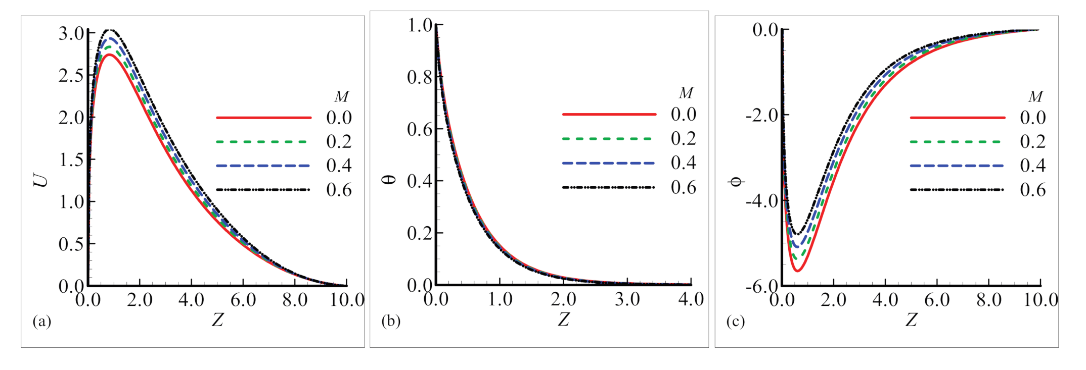
Figure 15.
Physical effects on quantities
and versus Pr, when = 0.1, 0.4, Q = 0.2, M = 0.2, = 0.2.

Table 1.
Physical effects on quantities
and versus , when remaining emerging parameters are constant.
Table 1.
Physical effects on quantities
and versus , when remaining emerging parameters are constant.
| Nb = 0.1 | Nb = 1.0 | Nb = 0.1 | Nb = 1.0 | Nb = 0.1 | Nb = 1.0 | |
|---|---|---|---|---|---|---|
| 0.1 | 0.28019 | 0.27897 | 0.65136 | 0.66346 | 0.39999 | 0.40399 |
| 1.0 | 1.34747 | 1.34216 | 0.70666 | 0.72635 | 0.67801 | 0.68116 |
| 2.0 | 1.16031 | 1.15575 | 0.68683 | 0.70445 | 0.61784 | 0.62109 |
| 3.0 | 0.16315 | 0.16272 | 0.63540 | 0.64245 | 0.23270 | 0.23778 |
Table 2.
Physical effects on quantities
and versus M, when remaining emerging parameters are constant.
Table 2.
Physical effects on quantities
and versus M, when remaining emerging parameters are constant.
| M = 0.2 | M = 0.8 | M = 0.2 | M = 0.8 | M = 0.2 | M = 0.8 | |
|---|---|---|---|---|---|---|
| 0.1 | 0.27951 | 0.27693 | 0.65533 | 0.65499 | 0.40432 | 0.40164 |
| 1.0 | 1.34503 | 1.08100 | 0.71309 | 0.68896 | 0.68082 | 0.60477 |
| 2.0 | 1.15823 | 0.57759 | 0.69259 | 0.66098 | 0.62072 | 0.45414 |
| 3.0 | 0.16290 | 0.09249 | 0.63772 | 0.63199 | 0.23703 | 0.15057 |
Table 3.
Physical effects on quantities
and versus , when remaining emerging parameters are constant.
Table 3.
Physical effects on quantities
and versus , when remaining emerging parameters are constant.
| Q = 0.1 | Q = 0.5 | Q = 0.1 | Q = 0.5 | Q = 0.1 | Q = 0.5 | |
|---|---|---|---|---|---|---|
| 0.1 | 0.27647 | 0.27777 | 0.69830 | 0.67952 | 0.40154 | 0.40235 |
| 1.0 | 1.33468 | 1.33918 | 0.75128 | 0.73451 | 0.67824 | 0.67935 |
| 2.0 | 1.14874 | 1.15285 | 0.73271 | 0.71513 | 0.61789 | 0.61911 |
| 3.0 | 0.16161 | 0.16216 | 0.68246 | 0.66294 | 0.23523 | 0.23600 |
Table 4.
Physical effects on quantities
and versus Sc, when remaining emerging parameters are constant.
Table 4.
Physical effects on quantities
and versus Sc, when remaining emerging parameters are constant.
| Sc = 0.3 | Sc = 0.7 | Sc = 0.3 | Sc = 0.7 | Sc = 0.3 | Sc = 0.7 | |
|---|---|---|---|---|---|---|
| 0.1 | 0.29190 | 0.28399 | 0.65416 | 0.65502 | 0.24685 | 0.34990 |
| 1.0 | 1.42701 | 1.37282 | 0.71728 | 0.71439 | 0.42843 | 0.59370 |
| 2.0 | 1.23893 | 1.18350 | 0.69594 | 0.69366 | 0.37666 | 0.53863 |
| 3.0 | 0.16793 | 0.16482 | 0.63709 | 0.63748 | 0.14962 | 0.20333 |
Publisher’s Note: MDPI stays neutral with regard to jurisdictional claims in published maps and institutional affiliations. |
© 2020 by the authors. Licensee MDPI, Basel, Switzerland. This article is an open access article distributed under the terms and conditions of the Creative Commons Attribution (CC BY) license (http://creativecommons.org/licenses/by/4.0/).
Share and Cite
MDPI and ACS Style
Khan, A.; Ashraf, M.; Rashad, A.M.; Nabwey, H.A. Impact of Heat Generation on Magneto-Nanofluid Free Convection Flow about Sphere in the Plume Region. Mathematics 2020, 8, 2010. https://doi.org/10.3390/math8112010
AMA Style
Khan A, Ashraf M, Rashad AM, Nabwey HA. Impact of Heat Generation on Magneto-Nanofluid Free Convection Flow about Sphere in the Plume Region. Mathematics. 2020; 8(11):2010. https://doi.org/10.3390/math8112010
Chicago/Turabian StyleKhan, Anwar, Muhammad Ashraf, Ahmed M. Rashad, and Hossam A. Nabwey. 2020. "Impact of Heat Generation on Magneto-Nanofluid Free Convection Flow about Sphere in the Plume Region" Mathematics 8, no. 11: 2010. https://doi.org/10.3390/math8112010
Note that from the first issue of 2016, this journal uses article numbers instead of page numbers. See further details here.