Company Value with Ruin Constraint in Lundberg Models

Abstract

In this note we study the problem of company values with a ruin constraint in classical continuous time Lundberg models. For this, we adapt the methods and results for discrete de Finetti models to time and state continuous Lundberg models. The policy improvement method works also in continuous models, but it is slow and needs discretization. Better results can be obtained faster using the barrier method for discrete models which can be adjusted for Lundberg models. In this method, dividend strategies are considered which are based on barrier sequences. In our continuous state model, optimal barriers can be computed with the Lagrange method leading to a backward recursion scheme. The resulting dividend strategies will not always be optimal: in the case without ruin constraint, there are examples in which band strategies are superior. We also develop equations for optimal control of dynamic reinsurance to maximize the company value under a ruin constraint. These identify the optimal reinsurance strategy in no action regions and allow for an interactive computation of the value function. We apply the methods in a numerical example with exponential claims.

1. Introduction

We consider a classical Lundberg model for the surplus $S\left(t\right)$ of an insurer at time t:

$$S\left(t\right)=s+ct-X_1-\dots -X_{N\left(t\right)},t\ge 0,$$

(1)

with initial surplus $s\ge 0,$ premium rate c and claim sizes $X,X_1,X_2,\dots$ which are iid. We will assume throughout that

$$X\mathrm{is}\text{non-atomic},\mathrm{i}.\mathrm{e}.,\mathbb{P}\{X=x\}=0\mathrm{for}\mathrm{all}x\ge 0.$$

The claims arrival process $N\left(t\right)$ is a homogeneous Poisson process with constant intensity $\lambda$. We always assume the net profit condition $c>\lambda E\left[X\right]$ which guarantees that $\tau =inf\{t:S(t)<0\}$ is infinite with positive probability, i.e., the ruin probability $\psi \left(s\right)=\mathbb{P}\{\tau <\infty |S\left(0\right)=s\}<1,$ and on $\{\tau =\infty \}$ we have $S\left(t\right)\to \infty .$

For a discount rate $\delta >0$ we compute the value of the insurance company as the expected discounted future sum of dividends:

$$V\left(s\right)=\underset{D}{sup}\left\{E\left[{\int }_0^{\infty }{e}^{-\delta t}dD\left(t\right)|S\left(0\right)=s\right]\right\},$$

(2)

where the supremum is taken over all predictable dividend strategies with total payment $D\left(t\right)$ up to time $t.$ We always assume that no dividends are paid at or after ruin.

For a given dividend strategy $D,$ the ruin probability of the with dividend risk process is defined by

$${\psi }^D\left(s\right)=\mathbb{P}\{S\left(t\right)-D\left(t\right)<0\mathrm{for}\mathrm{some}t\ge 0|S\left(0\right)=s\}.$$

In this note we consider the company value with ruin constraint

$$V(s,\alpha )=\underset{D}{sup}\left\{E\left[{\int }_0^{\infty }{e}^{-\delta t}dD\left(t\right)|S\left(0\right)=s\right]:{\psi }^D\left(s\right)\le \alpha \right\}$$

(3)

which is defined for $s\ge 0$ with $\psi \left(s\right)\le \alpha \le 1.$

Dividend optimization with a ruin related constraint has been considered in several earlier papers: Albrecher and Thonhauser (2007), Hernandez et al. (2017) as well as Junca et al. (2018) deal with the time value of ruin. In these problems both objective functions are discounted which allows for explicit solutions.

Without a ruin constraint, the optimal dividend problem is often solved by a barrier strategy, i.e., there exists a constant $B^{*}\ge 0$ such that

$$\begin{array}{ccc}\hfill D\left(t\right)& =& \underset{0\le u\le t}{sup}{(S\left(u\right)-B^{*})}^{+},\hfill \end{array}$$

(4)

$$\begin{array}{ccc}\hfill V\left(s\right)& =& v\left(s\right)/v^{\prime }\left(B^{*}\right),s\le B^{*},\hfill \end{array}$$

(5)

$$\begin{array}{ccc}\hfill V\left(s\right)& =& V\left(B^{*}\right)+s-B^{*},s\ge B^{*},\hfill \end{array}$$

(6)

$$\begin{array}{ccc}\hfill B^{*}& =& \arg \min \{v^{\prime }\left(s\right),s\ge 0\},\hfill \end{array}$$

(7)

where $v\left(s\right)$ is the scale function given below. The corresponding with dividend process $S\left(t\right)-D\left(t\right)$ has certain ruin for each initial surplus $s$.

The optimal dividend strategy defining the company value can also be a band strategy in which two or more bands exist: these are disjoint closed intervals $[a_i,b_i],i=1,\dots ,m,$ with $0=a_1<a_2<\dots <a_m$ in which no dividends are paid. The with dividends surplus process lives in the union of these intervals: dividends are paid at $b_i,$ and if the process drops below $a_i,$ then no dividends are paid when we reach a point in one of the intervals $[a_j,b_j],$ or dividends are paid such that the resulting surplus lies in the largest value $b_j$ below the surplus before dividend payment. For situations in which barrier strategies are optimal for spectrally negative Lévy processes see Loeffen (2008) and Loeffen and Renaud (2018).

For the characterization and computation of the value function and the corresponding optimal strategy see (Schmidli 2007, sct. 2.4). When the solution $v\left(x\right)$ of Equation (12) with $v\left(0\right)=1$ has a continuous derivative $v^{\prime }\left(x\right)$ with $v^{\prime }\left(x\right)$ decreasing for $x<B$ and $v^{\prime }\left(x\right)$ increasing for $x>B,$ then we have optimality of a barrier strategy, and $B=B^{*}$ is the value of this barrier.

For initial surplus below $b_1,$ the upper bound of the first band, a barrier strategy is optimal, since the process stays in the interval $[a_1,b_1].$ The problem of optimality for barrier strategies is unsolved in the case with ruin constraints. There, it might be possible to have optimal dividend strategies which are band strategies with bands depending on the allowed ruin probability $\alpha$.

In our numerical example we checked for optimality of barrier strategies. Using the iteration method, we could not find a second band in the range $s\le 50,$ for exponentially distributed claims.

For dividend strategies $D\left(t\right)$ representing (or approximating) the company value with ruin constraint, the with dividend process $S\left(t\right)-D\left(t\right)$ may not be bounded, i.e.,

$$\mathbb{P}\{\underset{t}{sup}[S\left(t\right)-D\left(t\right)]<\infty \}=0,$$

for otherwise we would have certain ruin which is excluded when $\alpha <1.$ With dividend processes which are unbounded can be obtained, e.g., with linear barriers (see Albrecher et al. (2005) and Gerber (1981)).

Remark 1.

With barriers

$$B\left(t\right)=at+b,t\ge 0,0<a<c,b\ge 0,$$

at time t the amount exceeding $B\left(t\right)$ is paid out as dividend. We write $U(s,a,b)$ for the dividend value of these strategies and $\psi (s,a,b)$ for the corresponding ruin probability. In our numerical example below (exponential claims with mean 1, premium rate 2 and discount rate 0.03) the dividend value $U(s,a,b)$ is considerably smaller than our numerical values for $V(s,\alpha )$ whenever $\psi (s,a,b)\le \alpha .$

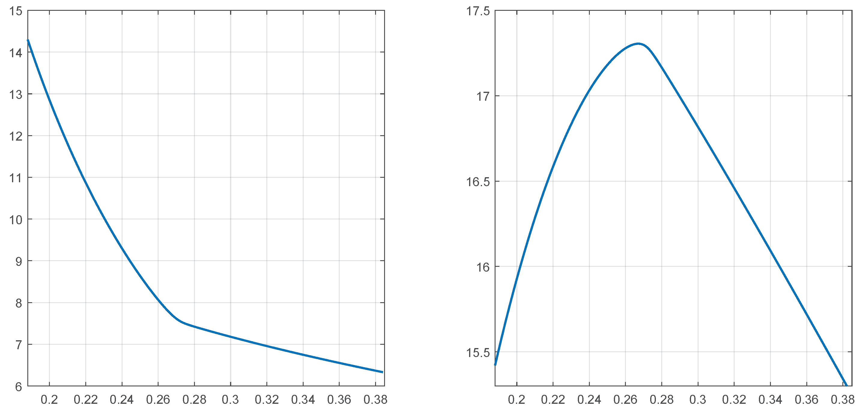
For this we consider the surplus $s=$ 2 and the allowed ruin probability $\alpha =$ 0.2. For 0 $<a<c$ we choose $b=b\left(a\right)>$ 0 such that $\psi (s,a,b)$ equals $\alpha .$ The company value computed with the barrier method equals $V=V(s,\alpha )=$ 20.15151719. Since for all $a,b>$ 0 we have $U(s,a,b)<v\left(s\right)/v^{\prime }\left(b\right)$ which is the unconstrained dividend value for a barrier b, we obtain from

$$v\left(2\right)/v^{\prime }\left(6.35\right)=20.0832891\mathrm{and}v\left(2\right)/v^{\prime }\left(14.2\right)=20.1146463$$

that U(2,a,b(a)) < V for b(a) < 6.35 and b(a) > 14.2. For a = 0.188 we obtain b(a) = 14.2955096, so U(2,a,b(a)) < V for $a\le$ 0.188. For a = 0.385 we obtain $b\left(a\right)=$ 6.322805359, so U(2,a,b(a)) < V for $a\ge$ 0.385. The interval 0.188 $\le a\le$ 0.385 was checked with step size 0.001. We found a maximum of the corresponding $U(s,a,b(a\left)\right)$ values of 17.304735 at a = 0.267. The curves of $b\left(a\right)$ and U(2,a,b(a)) are shown in Figure 1. For the computation we used the formulas in Gerber (1981) (18), (20), (23), (24), (27) for $\psi (s,a,b)$ and (20), (48)–(51) for $U(s,a,b).$ We checked our source code with the numerical results in Albrecher et al. (2005).

2. Methods

2.1. Policy Improvement without Bellman Equation

This method is conceptually and formally equivalent to the iteration method described in Hipp (2017). We repeat the iteration procedure for the sake of completeness: we start with an appropriate initial value function $V_0(s,\alpha )$ such as

$$V_0(s,\alpha )=0$$

or

$$\begin{array}{ccc}\hfill V_0(s,\alpha )& =& V(s-s(\alpha \left)\right),s\ge s\left(\alpha \right),\hfill \\ \hfill V_0(s,\alpha )& =& 0,s<s\left(\alpha \right),\hfill \\ \hfill \alpha & =& E\left[\psi \right(s\left(\alpha \right)-Y\left)\right].\hfill \end{array}$$

Here, Y is the claim causing ruin when dividends are paid using a dividend strategy with barrier $B^{*}.$ The second initial function is the dividend value for the strategy which pays out the total surplus above the barrier $B^{*}+s\left(\alpha \right)$ and stops paying dividends forever when the surplus is below the value $s\left(\alpha \right).$ For the iteration we define

$$\begin{array}{ccc}\hfill V_{n+1}(s,\alpha )& =& \underset{B\ge s}{max}\left\{W(s,B)V_n(s,a\left(B\right))\right\}\hfill \end{array}$$

(8)

$$\begin{array}{ccc}\hfill V_{n+1}(s,\alpha )& \ge & V_{n+1}(s-1,\alpha )+1\mathrm{if}\psi (s-1)\le \alpha ,\hfill \end{array}$$

(9)

$$\begin{array}{ccc}\hfill \alpha & =& p(s,B)+(1-p(s,B\left)\right)a\left(B\right).\hfill \end{array}$$

(10)

Here, $p(s,B)$ is the probability that the without dividend process $S\left(t\right)$ falls below zero before reaching $B,$ and $W(s,B)$ is the discounting factor $E[exp(-\delta \tau (s,B)\left)\right]$ for $\tau (s,B)$ the waiting time to reach B from s before ruin. This device produces a monotone sequence of functions $V_n$ which converge to a function which is a possible candidate for the value function $V(s,\alpha ).$ The first Equation (8) covers the case in which no dividends are paid before reaching $B,$ while Equation () allows for immediate dividend payment at surplus $s.$ The functions $p(s,B)$ and $W(s,B)$ can be written with the survival function and the scale function given below.

2.2. Barrier Method

For the construction of optimal dividend strategies the barrier method has been used for time and state discrete models in Hipp (2018). There, an increasing sequence of barriers had been selected at which dividends are paid, and the dividend value as well as th corresponding ruin probability were computed. We adjust this for the continuous Lundberg model and use an optimal selection of barriers which is based on the Lagrange multiplier method.

The two fundamental ingredients for the Lundberg model are the survival probability $f\left(s\right)=1-\psi \left(s\right)$ which satisfies $f\left(s\right)=0$ for $s<0$ and the equation

$$\lambda E[f(s-X)-f\left(s\right)]+c{f}^{\prime }\left(s\right)=0,$$

(11)

as well as the scale function $v\left(s\right)$ which is the unique solution of the equation

$$-\delta v\left(s\right)+\lambda E[v(s-X)-v\left(s\right)]+c{v}^{\prime }\left(s\right)=0,$$

(12)

satisfying $v\left(s\right)=0,s<0,$ and $v\left(0\right)=1.$

We also consider the functions $g\left(s\right)=E\left[f\right(s-X\left)\right]$ and $w\left(s\right)=E\left[v\right(s-X\left)\right].$ With formulas (11) and (12) these can be computed as

$$\begin{array}{ccc}\hfill g\left(s\right)& =& \lambda f\left(s\right)-c{f}^{\prime }\left(s\right),s\ge 0,\hfill \end{array}$$

(13)

$$\begin{array}{ccc}\hfill w\left(s\right)& =& (\lambda +\delta )v\left(s\right)-c{v}^{\prime }\left(s\right),s\ge 0.\hfill \end{array}$$

(14)

Many ruin related quantities can be expressed via $f\left(s\right)$, and most dividend values are connected with $v\left(s\right).$ Examples are first entry probabilities (before ruin) and discount factors corresponding to the time of first entry (see Hipp (2018)). So, e.g., the functions $p(s,B)$ and $W(s,B)$ are given by

$$p(s,B)=f\left(s\right)/f\left(B\right)\mathrm{and}W(s,B)=v\left(s\right)/v\left(B\right).$$

(15)

The Equations (11) and (12) have solutions with continuous first derivative when the claim size distribution is non-atomic. All solutions of (11) vanishing for $s<0$ are proportional. The same is true for Equation (12).

Fix an initial surplus $s>0$ and an allowed ruin probability $\alpha$ with $\psi \left(s\right)<\alpha \le 1.$ We first define the running ruin probabilities introduced in Hipp (2017) for a dividend strategy D which is defined via a finite non-decreasing sequence $s<B_0<B_1<\dots <B_n$: whenever we reach $B_i,i\le n,$ all incoming premia are paid out as dividends until the next claim happens. When the surplus reaches $B_n,$ we pay out all premia as dividends until the next claim happens, and then we stop dividend payment forever. For $0\le x<B_0$ the ruin probability ${\psi }^D\left(x\right)$ of the (with dividend) risk process $S\left(t\right)-D\left(t\right)$ is proportional to $\psi \left(x\right)$, and ${\psi }^D\left(s\right)=\alpha$ implies that it can be written as

$${\psi }^D\left(x\right)=1-{\gamma }_0+{\gamma }_0\psi \left(x\right),{\gamma }_0=\frac{1-\alpha }{1-\psi \left(s\right)}.$$

(16)

These running allowed ruin probabilities had been introduced in Hipp (2018) for a discrete model. Let $B_i$ be one of the barrier levels at which all premia are paid out as dividends. Then the corresponding running ruin probability $r_i\left(x\right),x\le B_i$ after hitting $B_i$ has the form

$$1-r_i\left(x\right)={\gamma }_i(1-\psi \left(x\right))={\gamma }_{i}f\left(x\right).$$

We leave level $B_i$ at the first claim during dividend payment. The ruin probability $r_{i+1}\left(x\right)$ after leaving the level $B_i$ and before hitting $B_{i+1}$ is also of the above form with ${\gamma }_{i+1}$ derived from $r_i\left(B_i\right)=E\left[r_{i+1}(B_i-X)\right]={\gamma }_{i}f\left(B_i\right)={\gamma }_{i+1}g\left(B_i\right)$ or

$${\gamma }_{i+1}={\gamma }_i\frac{f\left(B_i\right)}{g\left(B_i\right)}.$$

The ruin probability ${\psi }^D\left(x\right)$ for the with dividend process $S\left(t\right)-D\left(t\right)$ satisfies ${\psi }^D\left(s\right)\le \alpha$ whenever

$${\gamma }_n=\underset{i}{max}{\gamma }_i\le 1.$$

Lemma 1.

For fixed surplus $s\ge$ 0 and allowed ruin probability 0 $<\alpha \le$ 1 let $s<B_0<B_1<\dots$ be an infinite sequence with $B_i\to \infty .$ Assume that the corresponding factors ${\gamma }_i$ converge to 1. Then ${\psi }^D\left(s\right)=\alpha ,$ where D is the dividend strategy which pays dividends on the barrier levels $B_i.$

Proof. 

The survival probability $1-{\psi }^D\left(s\right)$ is the probability that from surplus s we reach $B_0,$ after leaving $B_0$ at a claim we reach $B_1$ and so on. For $B\ge x\ge 0$ let $p(x,B)$ be the probability that the without dividend process $S\left(t\right)$ starting at x will reach B before ruin. Then

$$p(x,B)=\frac{f\left(x\right)}{f\left(B\right)}.$$

The events $A_i,i=1,2\dots$ that after dividend payment at $B_{i-1}$ the surplus will reach $B_i$ are independent and have probability

$$E\left[p(B_{i-1}-X,B_i)\right]=\frac{g\left(B_{i-1}\right)}{f\left(B_i\right)}.$$

The event $A_0$ that $S\left(t\right)$ starting at s will reach $B_0$ has probability

$$\frac{f\left(s\right)}{f\left(B_0\right)}.$$

For $i\ge 0$ we have

$$\frac{g\left(B_i\right)}{f\left(B_{i+1}\right)}=\frac{{\gamma }_i}{{\gamma }_{i+1}}\frac{f\left(B_i\right)}{f\left(B_{i+1}\right)}$$

and so we obtain the survival probability

$$\frac{f\left(s\right)}{f\left(B_0\right)}\prod _{i=0}^{\infty }\frac{g\left(B_i\right)}{f\left(B_{i+1}\right)}=f\left(s\right){\gamma }_0=1-\alpha .$$

(17)

☐

With a finite sequence $s<B_0<B_1<B_2<\dots <B_n$ we represent a dividend strategy in which dividend payment is stopped forever when the surplus leaves $B_n,$ i.e., ${\gamma }_{n+1}=1$ and $B_{n+1}=\infty .$ The survival probability after reaching $B_n$ equals $g\left(B_n\right).$ For this strategy we obtain the survival probability

$$1-{\psi }^D\left(s\right)=\frac{f\left(s\right)}{f\left(B_0\right)}\prod _{i=0}^{n-1}\frac{g\left(B_i\right)}{f\left(B_{i+1}\right)}g\left(B_n\right)=(1-\alpha )/{\gamma }_n\ge 1-\alpha .$$

The present value of dividends paid on a barrier $B_i$ does not depend on $i,$ it is

$$A={\int }_0^{\infty }{\int }_0^{t}cexp(-\delta u)\lambda exp(-\lambda t)dt=\frac{c}{\lambda +\delta }.$$

This dividend value is discounted to the time at which $B_i$ is visited first. The discount factor for the time spent at barrier level $B_i$ equals

$$C={\int }_0^{\infty }\lambda exp(-\lambda t)exp(-\delta t)dt=\frac{\lambda }{\lambda +\delta }.$$

(18)

The discount factor for the time between leaving $B_i$ and hitting $B_{i+1}\ge B_i$ equals

$$G_i:=E[w\left(B_i\right)/v\left(B_{i+1}\right)]=\frac{\lambda +\delta }{\lambda }\frac{v\left(B_i\right)}{v\left(B_{i+1}\right)}-\frac{c}{\lambda }\frac{v^{\prime }\left(B_i\right)}{v\left(B_{i+1}\right)}.$$

(19)

The dividend value for a strategy D with barriers $B_0,B_1,\dots ,B_n$ satisfying

$$s\le B_0\le B_1\le \dots \le B_n$$

is given by

$$V^D\left(s\right)=Aw\left(s\right)/w\left(B_0\right)\sum _{i=0}^n{U}_i,$$

(20)

where $U_0=1$ and $U_{i+1}=C{G}_i{U}_i.$ The present value of dividends paid at level $B_0$ equals $Av\left(s\right)/v\left(B_0\right).$ The present value for dividends paid at level $B_1$ equals $Av\left(s\right)/v\left(B_0\right)C{G}_0,$ and the next barrier level contributes

$$Av\left(s\right)/v\left(B_0\right)C^2{G}_0{G}_1,$$

and so on. For equal barriers $B_i=M$ we easily obtain that for $s\le M$ and with $G=G_i$

$$V\left(s\right)=A\frac{v\left(s\right)}{v\left(M\right)}\frac{1}{1-CG}=\frac{v\left(s\right)}{v^{\prime }\left(M\right)}$$

which is the well known correct value (compare with Renaud and Zhou (2007)).

We first consider dividend strategies which have only one barrier B at which dividends are paid a finite number of times. This means that barriers are paid at $B_0=B,\dots ,B_K=B,$ and after paying dividends on barrier level $BK+1$ times we stop paying dividends forever. The barrier B can be chosen such that the allowed ruin probability is exact, and the corresponding dividend value can be given explicitly.

Lemma 2.

For any given pair $s,\alpha$ with $\psi \left(s\right)<\alpha$ and $K\ge 1$ we can find B such that the above dividend strategy $D\left(t\right)$ yields the with dividend ruin probability $\mathbb{P}\left\{S\right(t)-D(t)<0\mathrm{for}\mathrm{some}t>0|S\left(0\right)=s\}=\alpha .$ The corresponding dividend value is

$$V=\frac{v\left(s\right)}{v^{\prime }\left(B\right)}\left(1-{\left(1-\frac{c{v}^{\prime }\left(B\right)}{(\lambda +\delta )v\left(B\right)}\right)}^{K+1}\right).$$

(21)

Proof. 

The with dividend survival probability is

$$\frac{f\left(s\right)}{f\left(B\right)}\prod _{i=1}^K\frac{g\left(B\right)}{f\left(B\right)}g\left(B\right)$$

(22)

which equals $1-\alpha$ whenever

$$1-\alpha =f\left(s\right){\left(\frac{g\left(B\right)}{f\left(B\right)}\right)}^{K+1},$$

so the appropriate choice for B is the solution of

$$\frac{g\left(B\right)}{f\left(B\right)}={\gamma }_0^{1/(K+1)}.$$

(23)

Equation (21) follows from (18)–(20). ☐

These one barrier strategies are clearly suboptimal: the dividend value converges to zero when $K\to \infty ,$ since the corresponding barriers converge to infinity. However, for moderate values of K the corresponding dividend values are surprisingly good. These can be used for barrier strategies for the tail of a finite barrier sequence $s<B_0<B_1<\dots <B_n:$ we choose K large enough such that the barrier B corresponding to ${\gamma }_n$ and K is larger than $B_n,$ and then the sequence of barriers in which $B_n$ is followed by K values of B has the exact allowed ruin probability. The same method applies to the choice of $B_0:$ if ${\gamma }_N<1$ then we can decrease $B_0$ to get an exact allowed ruin probability (and a slightly larger dividend value).

A manual search for good sequences of barrier sequences is tedious: we used

• linear sequences of the form $B_i=B_0+i\Delta ,i=1,\dots ,n,$
• sequences satisfying the recursion

  $$g\left(B_{i+1}\right)/f\left(B_{i+1}\right)=g\left(B_i\right)/f{\left(B_i\right)}^{\rho },i=0,\dots ,n-1,$$

  (24)
• barriers $s<B_0<\dots <B_n$ with small n which are selected manually.

Linear sequences produce dividend values which are almost optimal, and sequences from recursion (24) can do even better, but are still suboptimal. We come close to optimal results when, for large $N,$ we maximize the dividend value $V=G(B_0,\dots ,B_N)$ using the Lagrange multiplier method. The problem has a high dimension, but using the structure of the function G we could find some simplifications. As a first step, we look at a related but simpler problem.

Problem: 

For $N\ge 1$ and a smooth increasing function $F\left(u\right)$ maximize the function

$$G(u_0\dots ,u_N)=\sum _{n=0}^N\prod _{i=0}^{n}F\left(u_i\right)$$

under the constraint

$$u_0+u_1+\dots +u_N=R.$$

We start with the Lagrange system of equations

$$\frac{\partial G}{\partial u_k}=\sum _{n=k}^N\prod _{i=0}^{n}F\left(u_i\right)\frac{F^{\prime }\left(u_k\right)}{F\left(u_k\right)}=L,k=0,\dots ,N.$$

For $n=N$ we get

$$L=\prod _{i=0}^{N-1}F\left(u_i\right)F^{\prime }\left(u_N\right)$$

which leads to the recursive relations

$$\frac{F^{\prime }\left(u_{i-1}\right)}{F\left(u_{i-1}\right)}=\frac{F\left(u_i\right)\dots F\left(u_{N-1}\right)F^{\prime }\left(u_N\right)}{1+F\left(u_i\right)+F\left(u_i\right)F\left(u_{i+1}\right)+\dots +F\left(u_i\right)\dots F\left(u_N\right)}.$$

For the calculation of $u_{i-1}$ we would need that $F^{\prime }\left(u\right)/F\left(u\right)$ is monotone.

In our control problem we want to maximize the following term by the choice of barriers $B_0,B_1,\dots ,B_N:$ with $F\left(x\right)=w\left(x\right)/v\left(x\right)$ and $Z\left(x\right)=1/v\left(x\right)$

$$G(B_0\dots ,B_N)=\frac{V}{Av\left(s\right)}=Z\left(B_0\right)+DF\left(B_0\right)Z\left(B_1\right)+D^{2}F\left(B_0\right)F\left(B_1\right)Z\left(B_2\right)+\dots +D^{N}F\left(B_0\right)\dots F\left(B_{N-1}\right)Z\left(B_N\right).$$

As in the above problem, we fix $B_N$ and use the Lagrange equations with a multiplier L and $H\left(x\right)=g\left(x\right)/f\left(x\right)$

$$\frac{\partial }{\partial B_i}G(B_0\dots ,B_N)=L{H}^{\prime }\left(B_i\right),i=0,\dots ,N.$$

(25)

With $i=N$ we get a formula for $L:$

$$F\left(B_0\right)\dots F(B_{N-1}{Z}^{\prime }\left(B_N\right)=H^{\prime }\left(B_N\right).$$

(26)

Our function $G\left(B\right)$ allows for the following simplification: for $i=0,\dots ,N-1$ the barrier $B_i$ solves

$$\begin{array}{ccc}\hfill A_1{H}^{\prime }\left(x\right)F\left(x\right)& =& Z^{\prime }\left(x\right)+A_2{F}^{\prime }\left(x\right),\hfill \end{array}$$

(27)

$$\begin{array}{ccc}\hfill A_1& =& C^{N-i}F\left(B_i\right)...F\left(B_{N-1}\right)Z^{\prime }\left(B_N\right)H^{\prime }\left(B_i\right)/H^{\prime }\left(B_N\right),\hfill \end{array}$$

(28)

$$\begin{array}{ccc}\hfill A_2& =& CZ\left(B_{i+1}\right)+C^{2}F\left(B_{i+1}\right)Z\left(B_{i+2}\right)+...+C^{N-i}F\left(B_{i+1}\right)...F\left(B_{N-1}\right)Z\left(B_N\right).\hfill \end{array}$$

(29)

Here, we first omit the factor $Av\left(s\right)$ and all terms in which $B_i$ does not occur, then we divide both sides by $F\left(B_0\right)\dots F\left(B_{i-1}\right)C^i.$ Equation (27) can be solved easily and quickly using Newton or the false position (regula falsi) method.

Some care is needed since the method has some uncommon features: We start with the last barrier $B_N$ which has practically no impact on the value of the company or the ruin probability, but in the recursion it determines all barriers. If we increase a large N by 1, then the company value as well as the corresponding ruin probability will change a lot, since we add a new first barrier which has a major impact on both numbers. Finally, we want to maximize $G(x_0,\dots ,x_N)$ under the constraint $s\le x_0\le \dots \le x_N.$ Nevertheless, the method is stable and accurate, even with the numerical precision of MatLab, and it produces admissible solutions. For $N=200$ we obtain $B_0=12.061058869$ and $V(2,0.2)=20.15151719.$

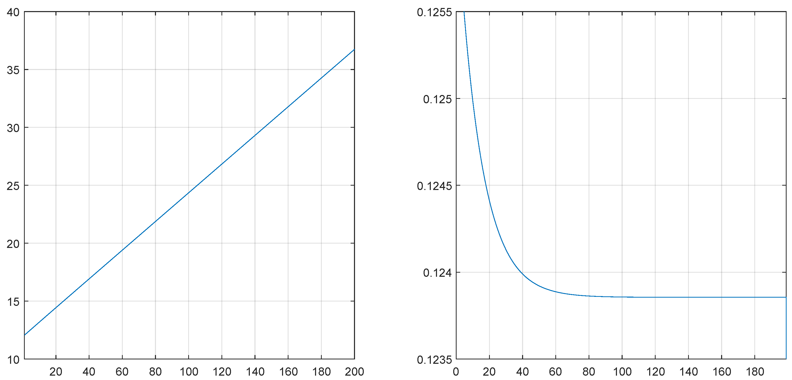
A plot of the resulting optimal barriers $B_0,\dots ,B_N$ in Figure 2 explains the good performance of linear sequences: the optimal sequences $B_0,\dots ,B_N$ are not linear but almost linear. Figure 2 left and right shows the optimal sequences and their increments in the example considered below.

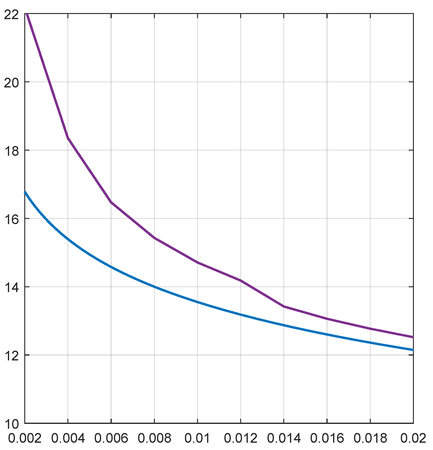
In dividend control problems, optimal strategies can often be characterized by a single barrier function $M\left(\beta \right),0<\beta \le 1,$ which identifies the optimal barriers for arbitrary initial surplus s and allowed ruin probability $\alpha :$ we start paying dividends whenever the with dividend process $S\left(t\right)-D\left(t\right)$ and the allowed running ruin probability $\alpha \left(t\right)$ hit $M\left(\beta \right),$ i.e., when $M\left(\alpha \right(t\left)\right)=S\left(t\right)-D\left(t\right).$ Notice that the optimal sequences $B_i$ and the corresponding running ruin probabilities $a_i\left(B_i\right)$ are points on the curve $M\left(\beta \right),$ i.e.,

$$M\left(a_i\left(B_i\right)\right)=B_i.$$

Figure 3 shows the function $M\left(\beta \right)$ at the points $\beta$ at which $M\left(\beta \right)=B_i,$ as well as the corresponding curve for the iteration method with

$$M\left(\beta \right)=min\{s:V_s(s,\beta )=1\}.$$

The curves should coincide; however, the second curve shows edges and higher values which are due to the discretization of s and $\alpha .$ The curves are plotted for $0<\beta \le 0.02$ only because of $a_0\left(B_0\right)=0.020859.$

2.3. Reinsurance Control for Company Value with Ruin Constraint

Many problems in stochastic control are solved via the well known Hamilton-Jacobi-Bellman equation. It is written for the value function of the given control problem reflecting the dynamics of the underlying stochastic model and the influence of control variables on these dynamics.

The case of a company value without ruin constraint is easy. We have a set of possible reinsurance contracts $g(x,a),0\le g(x,a)\le x,a\in A,$ which describe the risk sharing at a claim of size X between insurer (paying $g(X,a)$) and reinsurer (paying $X-g(X,a)$), and we have a reinsurance premium $h\left(a\right)$ for contract $a.$ Then the Hamilton-Jacobi-Bellman equation for the candidate solution $v\left(s\right)$ satisfying $v\left(0\right)=1$ reads

$$\underset{a\in A}{sup}\left(-\delta v\left(s\right)+\lambda E[v(s-g(X,a))-v\left(s\right)]+(c-h\left(a\right))v^{\prime }\left(s\right)\right)=0.$$

(30)

The optimal dividend strategy is of barrier type if $v^{\prime }\left(s\right)$ is decreasing in $[0,B]$ and increasing in $[B,\infty ),$ and in this case B is the barrier. We let $V\left(s\right)=v\left(s\right)/v^{\prime }\left(B\right)$ when $s\le B$ while $V\left(s\right)=V\left(B\right)+s-B$ for $s>B.$ On the no action region $[0,B)$ we can restrict the possible reinsurance contracts to $A_c=\{a\in A:h\left(a\right)<c\},$ and then

$$V^{\prime }\left(s\right)=\underset{a\in A_c}{inf}\frac{(\lambda +\delta )V\left(s\right)-\lambda E\left[V\right(s-g(X,a)\left)\right]}{c-h\left(a\right)}.$$

(31)

The optimal reinsurance strategy in the no action region is given by the minimizer $a^{*}\left(s\right)$ in (31). This approach solves our control problem: Equation (30) is homogeneous, the set of solutions has dimension 1, and the optimal reinsurance strategy is unique. Furthermore, from (30) we get an iteration producing a non-decreasing sequence of functions converging to $V\left(s\right)$. For reinsurance control to minimize the ruin probability—which uses quite similar techniques—see Hipp and Vogt (2003) as well as Dickson and Waters (2006).

The situation of a company value with ruin constraint is more complex. We can simplify the problem by fixing a sequence of barriers $s_0\le B_0<\dots <B_N$ on which dividends are paid, and use the running ruin probability ${\psi }_n\left(x\right)$ valid for $x<B_n$ after visiting the barriers $B_0,\dots ,B_{n-1}.$ Then the function $V\left(x\right)=V(x,{\psi }_n\left(x\right))$ satisfies Equation (30) above. This implies that the optimal reinsurance strategy for maximizing the company value with ruin constraint equals $a^{*}\left(x\right)$ for $0\le x<B_n,$ i.e., the same strategy as without ruin constraint, as long as we are in the no action region. This holds generally when we are not on a barrier level, no matter how many barriers we have visited. With the Markov property we get a constant value for the reinsurance parameter on each single barrier. If the barriers and these parameters $a_i$ are fixed, then we can compute the corresponding dividend value with formula (20), where $W\left(s\right)$ is replaced by the candidate solution of

$$0=-\delta v\left(s\right)+\lambda E[v(s-g(X,a^{*}\left(s\right)))-v\left(s\right)]+(c-h\left(a^{*}\left(s\right)\right)v^{\prime }\left(s\right).$$

In addition, the ruin probabilities ${\varphi }_n\left(x\right)$ for the no action regions are computed under the optimal reinsurance strategy:

$$0=\lambda E[{\varphi }_n(s-g(X,a^{*}\left(s\right)))-{\varphi }_n\left(s\right)]+(c-h\left(a^{*}\left(s\right)\right){\varphi }_n^{\prime }\left(s\right).$$

The reinsurance strategies $a_i$ valid on the barriers were specified manually. Our first guess was $a_i=a^{*}\left(B_i\right),$ for which we would not have a jump in the optimal reinsurance strategy when reaching $B_i.$ However, in our numerical experiments we found that an optimal strategy uses more reinsurance during dividend payment. This is surprising since this at the same time reduces dividend payment.

In our numerical example we use these tools to manually construct a solution via the choice of a barrier sequence $B_i$ and contract parameters $a_i$ on these barriers. The corresponding dividend strategy pays the dividend rate $c-h\left(a_i\right)$ on the barrier $B_i,$ and the running ruin probabilities ${\varphi }_i\left(x\right)$ are concatenated via

$$E\left[{\varphi }_{i+1}(B_i-g(X,a^{*}\left(B_i\right)))\right]={\varphi }_i\left(B_i\right).$$

3. Numerical Example

We consider a Lundberg process with premium rate 2, exponential claims with mean 1, a claim frequency of 1, and the interest rate $\delta =0.03.$ Here we have explicit formulas for $f\left(s\right),g\left(s\right),v\left(s\right),w\left(s\right)$ and their derivatives:

$$\begin{array}{ccc}\hfill f\left(s\right)& =& 1-exp(-s/2)/2,\hfill \end{array}$$

(32)

$$\begin{array}{ccc}\hfill g\left(s\right)& =& E\left[f\right(s-X\left)\right]=1-exp(-s/2),\hfill \end{array}$$

(33)

$$\begin{array}{ccc}\hfill v\left(s\right)& =& (1-C)exp\left(a_{1}s\right)+Cexp\left(a_{2}s\right),\hfill \end{array}$$

(34)

$$\begin{array}{ccc}\hfill w\left(s\right)& =& EW\left[v(s-X)\right]=(1+\delta )v\left(x\right)-c{v}^{\prime }\left(s\right),\hfill \end{array}$$

(35)

$$\begin{array}{ccc}\hfill a_1& =& 0.02917305718455,\hfill \end{array}$$

(36)

$$\begin{array}{ccc}\hfill a_2& =& -0.5141730571845,\hfill \end{array}$$

(37)

$$\begin{array}{ccc}\hfill C& =& -0.894138984281798,\hfill \end{array}$$

(38)

$$\begin{array}{ccc}\hfill M& =& 9.180097300194138.\hfill \end{array}$$

(39)

We take $s=2$ and $\alpha =0.2.$ The ruin probability without dividend payment is

$$\psi \left(s\right)=0.18393972$$

(40)

which is quite close to $\alpha .$

The iteration method produces—with discretization $1/100$ for s and $1/500$ for $\alpha$ and 100 repetitions—the value $V(2,0.2)=19.8246037.$ The computation time for one iteration was 240–260 cpu seconds. Additional iterations change little, the value for 150 iterations is $19.82804494.$ We used the initial function

$$\begin{array}{ccc}\hfill V_0(s,\alpha )& =& 0\mathrm{if}s<s\left(\alpha \right),\hfill \end{array}$$

(41)

$$\begin{array}{ccc}\hfill V_0(s,\alpha )& =& V_0(s-s\left(\alpha \right)),s\ge s\left(\alpha \right),\hfill \end{array}$$

(42)

where $\alpha =E\left[\psi \right(s\left(\alpha \right)-Y\left)\right]$ and Y is the claim causing ruin in the risk process with barrier dividend payment. For exponential claim sizes, Y has the same distribution as X. The dividend value corresponds to a strategy which pays dividends without a constraint until the surplus drops below $s\left(\alpha \right)$. The unconstrained dividend value equals $V(2,1)=22.11840639.$ This and later values show that ruin constraints are rather cheap.

We next compute the dividend function with the barrier method. With the following linearly increasing barrier levels we obtain $V(2,0.2)=20.0750017795$ (using MAPLE and 50 digits accuracy):

$$\begin{array}{ccc}\hfill B_0& =& 11.47909729919,\hfill \end{array}$$

(43)

$$\begin{array}{ccc}\hfill B_1& =& 11.648050776,\hfill \end{array}$$

(44)

$$\begin{array}{ccc}\hfill B_i& =& B_{i-1}+0.16895347669,i=2,\dots ,400.\hfill \end{array}$$

(45)

These barriers were obtained via a simple but tedious manual search. The first barrier $B_0$ is chosen to yield an exact allowed ruin probability $\alpha .$ The difference between this result and the result in the iteration method is due to discretization of s and $\alpha .$

The second search was done with barriers for which $log(g\left(B_{i+1}\right)/f\left(B_{i+1}\right))=\rho log(g\left(B_{i+1}\right)/f\left(B_{i+1}\right)),i\ge 1.$ The choice of $\rho =0.9299,B_0=11.41895,B_1=11.9442$ produced the dividend value $V=20.12254329.$ This is better than the best value with linearly increasing barriers, but still not optimal, and it is unclear why this definition of the $B_i$ produces a close to optimal company value.

Of course, for optimal barriers one should try the Lagrange method since it characterizes a local maximum of the function $G(B_0,\dots ,B_N)$ under a constraint $H\left(B_0\right)+\dots +H\left(B_N\right)=R,$ where $H\left(x\right)=log\left(g\right(x)/f(x\left)\right)$ and $R=log\left({\gamma }_0\right).$ Since the problem is high dimensional and the function is highly non-linear, the Lagrange method was not the first choice for the optimization. However, it surprisingly works with the backward recursion described above. With $N=200$ we obtain the dividend value $V=20.15151719.$ The first two barriers are $B_0=12.06105887$ and $B_1=12.18704856.$ The optimal barriers go up to $B_N=36.80050963.$

For the control of reinsurance we consider unlimited XL-reinsurance which is parametrized by a threshold $M\in [0,\infty ]$ and defined via

$$g(x,M)=min(x,M),$$

i.e., the reinsurer pays the amount of the claim exceeding $M.$ The reinsurance premium is assumed of the form

$$h\left(M\right)=\lambda c\rho E\left[{(X-M)}^{+}\right]/E\left[X\right],$$

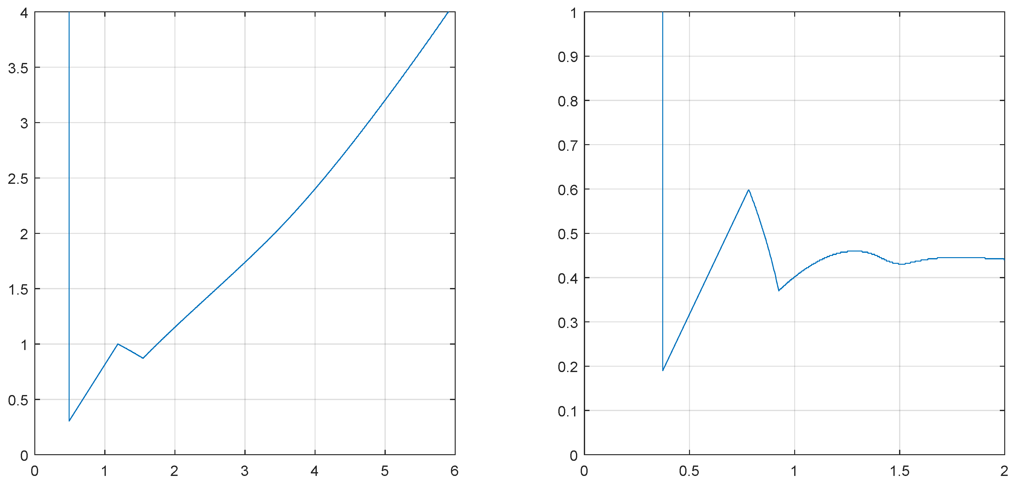
where the loading factor $\rho =1.2>1$ avoids an ill posed problem. We first compute the optimal reinsurance strategy to maximize the unconstrained company value $V\left(s\right).$ The optimal reinsurance strategy for the unconstraint company value is given in Figure 4 which shows that

• for small surplus no reinsurance is written, $M\left(s\right)=\infty$,
• then $M\left(s\right)=s$ is optimal, which guarantees the payment of the next claim, and finally
• $M\left(s\right)$ is below s but still increasing (in contrast to the case of ruin probabilities).

We use these facts—which we could see in a complete search—also in our computer code; this speeds up a lot. In the region without reinsurance, the candidate solution $v\left(s\right)$ is the function $W\left(s\right)$ above. In the range where $M\left(s\right)=s,$ the defining equation reads

$$0=[(\lambda +\delta )v\left(s\right)-\lambda v\left(0\right)-(c-h\left(s\right))v^{\prime }\left(s\right).$$

We obtain a minimum of $v^{\prime }\left(s\right)$ at $M=7.85,$ and a company value of $V\left(2\right)=v\left(2\right)/v^{\prime }\left(M\right)=25.124375$. These values are computed with MatLab and a discretization step size $1/500$ for s, and $1/1.000$ for $\alpha ,$ so the accuracy is not too bad. The ruin probability under this dynamic reinsurance strategy is $\varphi \left(2\right)=0.0381551,$ much smaller than without reinsurance (see (40)). The minimal ruin probability with reinsurance is $\varphi \left(2\right)=0.018648.$ In the following we work with allowed ruin probability $\alpha =0.05$.

For $2=s<B_0<\dots <B_n$ we first used $a_i=M\left(B_i\right)$. The running ruin probabilities $a_i\left(x\right)$ are again of the form

$$a_i\left(x\right)=1-{\gamma }_i+{\gamma }_i\varphi \left(x\right),$$

with ${\gamma }_0=(1-\alpha )/(1-\varphi \left(s\right))$ and ${\gamma }_{i+1}={\gamma }_i(1-\varphi \left(B_i\right))/(1-E\left[\varphi (B_i-g(X,a_i))\right].$ As above, our choice of barriers satisfies the ruin constraint whenever ${\gamma }_n<1.$ The corresponding company value is given by

$$\begin{array}{ccc}\hfill V\left(s\right)& =& \frac{W\left(s\right)}{W\left(B_0\right)}\sum _{i=0}^n{A}_i{U}_i,\hfill \end{array}$$

(46)

$$\begin{array}{ccc}\hfill A_i& =& \frac{c-h\left(a_i\right)}{\lambda +\delta },\hfill \end{array}$$

(47)

$$\begin{array}{ccc}\hfill C& =& \lambda /(\lambda +\delta ),\hfill \end{array}$$

(48)

$$\begin{array}{ccc}\hfill G_i& =& E\left[W(B_i-g(X,a_i))\right]/W\left(B_{i+1}\right)\hfill \end{array}$$

(49)

$$\begin{array}{ccc}\hfill U_0& =& 1,U_{i+1}=C{G}_i{U}_i.\hfill \end{array}$$

(50)

The following

Table 1. Dividend values for five reinsurance strategies.

ReIns	${\mathit{B}}_0$	$\mathit{\beta }$	$\mathit{V}(2,0.05)$
A	$9.405$	$0.105$	23.7637
B	$9.43$	$0.104$	23.761297
C	$9.40487$	$0.104$	$23.765385$
D	$9.4$	$0.10437$	$23.768094$
E	$9.449$	$0.104$	$23.75439$

gives our manually maximized company values with linear barrier levels $B_i=B_0+i\beta$ for five different parameters $B_0,\beta$ and reinsurance contracts $a_i$ on the barrier levels $B_i:$ A: $a_i=M\left(B\left(i\right)\right),$ B: $a_i=M\left(B\left(i\right)\right)+0.2,$ C: $a_i=M\left(B\left(i\right)\right)-0.2,$ D: $a_i=M\left(B\left(i\right)\right)-0.7,$ and E: no reinsurance. For each case we show the optimal first barrier $B_0$ and the corresponding optimal $\beta .$

The largest company value in our experiments was case D with expensive reinsurance on the barrier levels. It produces the value

$$V(2,0.05)=23.768094.$$

If we stop reinsurance after 54 visited barriers and start with $B_0=9.38955,$ the reinsurance $a_i=M\left(B\left(i\right)\right)-1.1$ increases the company value to $23.7689406.$ This dividend value is certainly still not optimal and/or accurate, so the search could be continued. In addition, one should think about characterizations of optimal barrier levels $B_i$ and corresponding reinsurance contracts $a_i.$

In the Appendix folder you will find the source codes of our MatLab calculation for the iteration method (called Lundberg Model and Iteration), three MAPLE codes for the barrier method, Barrier1 for linear barriers $B_i,$ and Barrier2 for barriers with the multiplicative definition above, and GerberFormulas for computations with linear barriers. The code LagrangeM computs the optimal barrier sequence via the Lagrange multiplier approach. We also include three MatLab codes for reinsurance control: Reinsurance1 and Reinsurance2, executed in this order, produce the results in the table above. For further experiments it is convenient to generate the file Reinsurance500.mat; loading this file and running ReMatrix generates a workspace for Reinsurance2.

References

- Albrecher, Hansjörg, and Stefan Thonhauser. 2007. Dividend maximization under consideration of the time value of ruin. Insurance: Mathematics and Economics 41: 163–84. [Google Scholar] [CrossRef]
- Albrecher, Hansjörg, Jürgen Hartinger, and Robert F. Tichy. 2005. On the distribution of dividend payments and the discounted penalty function in a risk model with linear dividend barrier. Scandinavian Actuarial Journal 2005: 103–26. [Google Scholar] [CrossRef]
- Dickson, David C. M., and Howard R. Waters. 2006. Optimal dynamic reinsurance. ASTIN Bulletin 36: 415–32. [Google Scholar] [CrossRef]
- Gerber, Hans Ulrich. 1981. On the probability of ruin in the presence of a linear dividend barrier. Scandinavian Actuarial Journal 1981: 105–15. [Google Scholar] [CrossRef]
- Hernandez, Camilo, Mauricio Junca, and Harold Moreno-Franco. 2018. A time of ruin constrained optimal dividend problem for spectrally one-sided Lévy processes. Insurance: Mathematics and Economics 79: 57–68. [Google Scholar] [CrossRef] [Green Version]
- Hipp, Christian. 2018. Company value with ruin constraint in a discrete model. Risks 6: 1. [Google Scholar] [CrossRef]
- Hipp, Christian. 2017. Working Paper on Dividend Payment Under a Ruin Constraint. Available online: researchgate.net/publication/318983299_Working_paper_on_dividend_payment_under_a _ruin_constraint (accessed on 17 July 2018).
- Hipp, Christian, and Michael Vogt. 2003. Optimal dynamic XL-reinsurance for a compound Poisson risk process. ASTIN Bulletin 33: 193–207. [Google Scholar] [CrossRef]
- Junca, Mauricio, Harold Moreno-Franco, José Pérez, and Kazutoshi Yamazaki. 2018. Optimality of refraction strategies for a constrained dividend problem. arXiv, arXiv:1803.08492. [Google Scholar]
- Loeffen, Ronnie L. 2008. On optimality of the barrier strategy in de Finetti’s dividend problem for spectrally negative Lévy processes. Annals of Applied Probability 18: 1669–80. [Google Scholar] [CrossRef]
- Loeffen, Ronnie L., and Jean-François Renaud. 2009. De Finetti’s optimal dividends problem with an affine penalty function at ruin. Insurance: Mathematics and Economics 46: 98–108. [Google Scholar] [CrossRef]
- Renaud, Jean-François, and Xiaowen Zhou. 2007. Distribution of the present value of dividend payment in a Lévi risk model. Journal of Applied Probability 44: 420–27. [Google Scholar] [CrossRef]
- Schmidli, Hanspeter. 2007. Stochastic Control in Insurance. Heidelberg: Springer, ISBN 978-1-84800-003-2. [Google Scholar]
Figure 1.
Plots of (Left) and (Right).
Figure 2.
Optimal barriers: values (Left) and increments (Right).
Figure 3.
Universal barriers from the Lagrange method (lower) and the iteration (upper curve).
Figure 4.
Optimal threshold for company value (left) and ruin probability